Farrikh Alzami*![]() | Abu Salam
| Abu Salam![]() | Ifan Rizqa
| Ifan Rizqa![]() | Candra Irawan
| Candra Irawan![]() | Pulung Nurtantio Andono
| Pulung Nurtantio Andono![]() | Diana Aqmala
| Diana Aqmala![]() | Mila Sartika
| Mila Sartika![]()
© 2024 The authors. This article is published by IIETA and is licensed under the CC BY 4.0 license (http://creativecommons.org/licenses/by/4.0/).
OPEN ACCESS
The SME sector in Indonesia comprises 99.99% of businesses, employing 96.9% of the workforce and contributing 60.5% to GDP and non-oil exports. Despite their importance, SMEs face challenges including limited financial access, product hygiene concerns, and fluctuating demand. Accurate demand prediction is crucial for optimizing production, inventory, and resource allocation. SARIMAX and VAR models are commonly used for demand prediction, with SARIMAX proving more effective, especially when integrating weather data. Due to there are quite few literatures about SARIMAX is used at SMEs, in this study we utilized SARIMAX and VAR models with sales and weather data (average temperature and average humidity) from January to June 2023. SARIMAX with optimum parameters optimum parameters (d=1, D=1, p=2, q=3, P=2, Q=2, s=7) outperformed optimized VAR in predicting demand for food and beverage SMEs. SARIMAX obtained AIC 1070.11, MSE 80.393, MAE 7.513, RMSE 8.966 and reduced MSE by 86.35% compared to VAR. This research highlights the significance of accurate demand prediction for SMEs, emphasizing the importance of considering external factors like weather. Understanding and predicting demand patterns are vital for SMEs to make informed decisions and optimize operations efficiently.
demand prediction, SME, SARIMAX, VAR, food, weather data, temperature, humidity
Small and Medium-sized Enterprises (SMEs) refer to businesses with 1-4 employees, predominantly micro-enterprises [1]. Statistics from the Ministry of Cooperatives and SMEs in 2019 revealed a staggering 64,194,056 SMEs, constituting 99.99% of the business landscape and engaging 96.9% of the workforce [2]. These enterprises play a pivotal role in the economy, contributing 60.5% to the national GDP and 15.6% to non-oil exports, underscoring their crucial significance in the country's economic framework [3]. In addition, SMEs have proven to be resilient during economic downturns and have the potential to drive inclusive and sustainable development [4]. There are several challenges that faced by SME in Indonesia, such as: 1) limited access to financial capital and financing options [5], 2) product hygiene and environmental sanitation as COVID-19 outbreak, and 3) number of demand for their products and services [6].
In this research, demand prediction is crucial for SMEs for several reasons. Firstly, accurate demand prediction allows SMEs to optimize their production and inventory management. By forecasting future demand, SMEs can adjust their production levels and inventory levels accordingly, ensuring that they have the right number of products available to meet customer demand. This helps to minimize the risk of stockouts or excess inventory, which can lead to financial losses and inefficiencies in the supply chain [7]. Also, SMEs can ensure that they have the appropriate amount of ingredients, raw materials, and finished products to meet customer needs. This helps minimize wastage, optimize production efficiency, and reduce costs [8]. Secondly, demand prediction enables SMEs to plan their resource allocation effectively. By understanding the expected demand for their products, SMEs can allocate their resources, such as labor, raw materials, and equipment, in a more efficient and cost-effective manner. This helps to optimize the utilization of resources and improve overall operational efficiency [7]. Furthermore, demand prediction plays a crucial role in financial planning and management for SMEs [9]. Accurate demand forecasts provide valuable information for budgeting, cash flow management, and financial decision-making. SMEs can use demand forecasts to estimate their revenue and plan their expenses, ensuring that they have sufficient financial resources to meet customer demand and sustain their operations [10]. Thus, by accurately forecasting demand, SMEs can collaborate with suppliers, distributors, and logistics providers to ensure a smooth and efficient flow of goods and services. This helps to minimize lead times, reduce costs, and improve customer satisfaction [11].
Demand prediction algorithms for various industries and applications have been introduced, such as: SARIMAX and vector Auto Regression (VAR). SARIMAX, which stands for Seasonal Autoregressive Integrated Moving Average with Exogenous Regressors, is well-suited for handling the time-dependent nature of demand data and capturing seasonality [12], handle time-dependent nature of demand data, and incorporate exogenous variables, making it a valuable tool for accurate and comprehensive time series forecasting in demand prediction scenarios [13]. SARIMAX have been used in various fields, such as electricity demand forecasting [14], energy consumption forecasting [15], parking occupancy forecasting [16], infectious disease [17], international visitor arrival [18].
The Vector Autoregression (VAR) model is a valuable tool for demand prediction due to its ability to capture the dynamic interdependencies among multiple time series variables [19]. VAR models offer several advantages. Firstly, they allow for the simultaneous modeling of multiple related time series variables, which is essential in capturing the complex relationships and feedback mechanisms that exist within demand data [20]. Additionally, VAR models are well-suited for handling the time-dependent nature of demand data, as they can capture both short-term and long-term dynamics, making them particularly effective for short-term demand forecasting [21]. This capability enables the model to account for the interdependencies among different demand-related factors, such as pricing, marketing efforts, and external economic indicators, leading to more comprehensive and accurate forecasts. VAR also have been used in several fields in SME topics, such as: job creation [22], hotel demand uncertainty [19], tax cut for labor demand [23].
Weather data can play a significant role in demand prediction across several industries. By incorporating weather patterns into forecasting models, businesses may anticipate fluctuations in consumer behavior influenced by weather. For instance, in the retail sector, weather can impact consumer demand for specific items such as clothing [24], or food and beverages [25]. In agriculture, weather data is key for predicting crop yields which indirectly influence the supply and demand dynamics in agricultural markets [26]. The impact of weather on demand is seasonal and sometimes geographical. Hence, models like SARIMAX, which account for seasonal data, can be quite beneficial when used alongside weather data. When using VAR, the interdependencies between weather factors and demand can be captured. For instance, temperature might impact demand for a product linearly, while precipitation might have a non-linear impact.
Thus, in the context of SME, rather than VAR model, SARIMAX model has not been explicitly studied. Nevertheless, both VAR and SARIMAX model for SME topic, there are not many topics which using weather data for demand product prediction. Thus, in this research, we utilized transactions data from food and beverage SME with weather data from SME’s location. In the specific context of SMEs, SARIMAX and VAR models is utilized to forecast demand for their products. By incorporating relevant exogenous variables such as weather data, SARIMAX and VAR models can provide valuable insights into future demand patterns. This can help SMEs optimize their production, inventory management, and marketing strategies to meet customer demand effectively.
From the experiment, our research concluded that SARIMAX outperform the VAR in matter demand prediction for food and beverage SMEs supplied with weather data (temp avg and humidity avg) and obtained values for AIC 1070.11, MSE 80.393, MAE 7.513 and RMSE 8.966.
The remainder of this paper is organized as follows, section 2 briefly reviews SARIMAX and VAR. Section 3 describes the methods used. Section 4 provides the conducted experiment and discussion. Then, section 5 presents conclusions and future works.
SARIMAX stands for Seasonal AutoRegressive Integrated Moving Average with eXogenous variables. It's a type of time series model that combines autoregressive, differencing (I), and moving average operations, as well as accounting for seasonality (seasonal ARIMA) and exogenous variables. It's used for forecasting when data has a trend and/or a seasonal pattern, and when external, independent variables might influence the time series variable being forecasted. It expands on simpler models like AR and MA by including trends and seasonality, allowing for more accurate predictions in these complex contexts.
The components of SARIMAX are:
(1) Seasonal (S): SARIMAX accounts for seasonality in the data. Seasonal patterns occur when there are regular fluctuations or patterns in the data that repeat over specific periods.
(2) Autoregressive (AR): This component captures the relationship between a variable and its own lagged values. In other words, it models the relationship between an observation and several lagged observations (from previous time steps).
(3) Integrated (I): The "integrated" part of SARIMAX indicates the differencing of raw observations to make the time series stationary. Stationary time series have constant statistical properties over time, making them easier to model.
(4) Moving Average (MA): This component models the relationship between a variable and a residual error from a moving average model applied to lagged observations.
(5) Exogenous Regressors (X): SARIMAX allows for the inclusion of exogenous variables, which are external factors that can influence the time series being analyzed. These variables are not directly related to the time series but are believed to have an impact on it. Including exogenous regressors in the model can improve its forecasting accuracy, especially when there are known external factors affecting the time series.
And the equation for SARIMAX (p,d,q)(P,D,Q,s) can be seen as follows:
$\Theta(\mathrm{L})^{\boldsymbol{p}} \theta\left(\mathrm{L}^{\boldsymbol{s}}\right)^{\boldsymbol{P}} \Delta^{\boldsymbol{d}} \Delta_{\boldsymbol{s}}^{\boldsymbol{D}} y_t=\Phi(\mathrm{L})^{\boldsymbol{q}} \boldsymbol{\phi}\left(\mathrm{L}^{\boldsymbol{s}}\right)^{\boldsymbol{Q}} \Delta^{\boldsymbol{d}} \Delta_{\boldsymbol{s}}^{\boldsymbol{D}} \epsilon_t+\sum_{i=1}^n \beta_i x_t^i$ (1)
where, $y_t$ is given time series, $p$ is the number of time lags to regress on, $\epsilon_t$ is the noise at time $t, \beta$ is constant, $L$ is regular lag operator, $\Theta(\mathrm{L})^p$ are order $p$ polynomial function of $L$, $q$ is the number of time lags of error to regress on, $\phi$ is defined analogously to $\Theta$, $\Delta^d$ is integration operator where $d$ is the order of differencing used, $\Delta_s^D$ is seasonal differences of the time series where $s$ is the number of time lags comprising one full period of seasonality and $D$ order differencing which applied to seasonal lags. Then, $n$ exogeneous variables defined at each time step $t$, denoted by $x_t^i$ for $i \leq n$.
The reason SARIMAX is chosen due to: 1) SARIMAX models allow for the inclusion of exogenous variables, such as weather features, which can significantly impact demand patterns. By incorporating these variables, SARIMAX models can capture the influence of external factors on demand and improve the accuracy of predictions [27]; 2) SARIMAX models are well-suited for capturing seasonal patterns and autocorrelation in demand data. The seasonal and autoregressive components of SARIMAX models enable them to model and forecast demand accurately, especially when there are recurring patterns and dependencies in the data [28]; 3) SARIMAX models offer flexibility in terms of model specification and customization. They can be tailored to specific demand patterns and adjusted to incorporate different exogenous variables, allowing for a more precise and tailored demand prediction [13]; 4) SARIMAX models provide interpretable results, allowing for a better understanding of the underlying factors driving demand. The coefficients and parameters of SARIMAX models can provide insights into the relationships between demand and exogenous variables, aiding in decision-making and strategy development [13].
One potential weakness is the sensitivity of the model to the selection of its parameters, which may require careful tuning and optimization for different types of demand data [29]. Additionally, SARIMAX may be less effective when dealing with highly volatile or irregular demand patterns, as it relies on capturing and modeling the underlying time series components, which may be challenging in such cases [18].
Vector Autoregression (VAR) is a type of statistical modeling used in econometrics that captures the linear interdependencies among multiple time series. It allows each variable in the system to be a function of the lagged values of all other variables in the system, which makes it crucial in forecasting systems of interrelated time series variables. Essentially, each variable in a VAR is modeled as a linear combination of past values of itself and the past values of all other variables in the system. The primary advantage of VAR is its ability to model the dynamic relationships amongst multiple (typically economic) variables simultaneously.
The equation for vector autoregression can be seen as follows:
$y_t=c+A_1 y_{t-1}+A_2 y_{t-2}+\cdots+A_p y_{t-p}+\varepsilon_t$ (2)
where, $y_t$ is $k \times 1$ vector representing the variable at time $t$. $c$ is $k \times 1$ vector of constants. $A_1$, $A_2$, $\ldots$, $A_p$ are $k \times k$ matrices of coefficients representing the lagged values of the variables. $p$ is the order of the VAR model, indicating how many lagged values are included in the model. Then, $\varepsilon_t$ is $k \times 1$ vector representing the error term at time $t$.
Also, the reason VAR is chosen due to: 1) VAR models are capable of capturing the interdependencies and dynamic relationships among multiple variables simultaneously. This makes them suitable for demand prediction, where multiple factors can influence the demand patterns [19]; 2) VAR models allow for the analysis and forecasting of multiple variables together, considering their mutual interactions. This is particularly useful when there are feedback loops and interrelationships among the variables, which can affect demand dynamics [30]; VAR models can incorporate exogenous variables, such as economic indicators, which can have an impact on demand. By including these variables, VAR models can capture the influence of external factors on demand patterns and improve the accuracy of predictions [31]. One potential weakness of VAR is the challenge of estimating a large number of parameters, especially when dealing with high-dimensional data or a large number of variables. This can lead to increased computational complexity and potential issues related to overfitting, particularly when the number of observations is limited [32].
To obtain optimal parameter for SARIMAX we utilized Akaike Information Criterion (AIC). Then, for VAR, there are several considerations, such as Akaike Information Criterion (AIC), Bayesian Information Criterion (BIC), Final Prediction Error (FPE) and Hannan-Quinn Information Criterion (HQIC).
The Akaike Information Criterion (AIC) is a statistical tool utilized to assess how well a statistical model fits the data. It strikes a balance between the model's fit quality and its complexity, discouraging overly intricate models that might overfit the data. When applied to Vector Autoregression (VAR) models, AIC helps compare various models, aiding in the selection of the most suitable one for forecasting or analyzing complex time series data with multiple variables. A lower AIC value indicates a better trade-off between goodness of fit and model complexity. When comparing different VAR models, you would choose the model with the lowest AIC value, as it suggests that the model provides a good fit to the data without being overly complex. The AIC equation can be seen as follows:
$A I C=-2 \log (L)+2 p$ (3)
where, $L$ is the likelihood of the data given the model. It represents how well the model explains the observed data. Then, $p$ is the number of parameters in the VAR(p) model, which includes the autoregressive coefficients and the error variances.
The Bayesian Information Criterion (BIC) helps balance the goodness of fit of a model with its complexity, penalizing models with more parameters. The BIC penalizes the number of parameters more heavily than the AIC, which means that it tends to favor simpler models. A lower BIC value indicates a better trade-off between goodness of fit and model complexity. The BIC equation can be seen as follows:
$B I C=-2 \log (L)+p \times \log (n)$ (4)
In here, $n$ is the number of observations in the time series data.
The Final Prediction Error (FPE) is used to estimate the expected mean squared prediction error of a model. FPE provides a measure of forecast accuracy, penalizing complex models to avoid overfitting. Like AIC and BIC, a lower FPE value indicates a better trade-off between goodness of fit and model complexity. The FPE equation can be seen as follows:
$F P E=\left(\frac{n+p+1}{n-p-1}\right) \times\left|\widehat{\sum u}\right|^{-1}$ (5)
In here, $\widehat{\sum u}$ is the estimated residual covariance matrix of the VAR(p) model.
The Hannan-Quinn Information Criterion (HQIC) provides a trade-off between the goodness of fit of the model and its complexity. The HQIC incorporates a logarithmic term related to the sample size $(n)$ that penalizes the number of parameters in the model. Like AIC and BIC, a lower HQIC value indicates a better trade-off between goodness of fit and model complexity. The equation can be seen as follows:
$H Q I C=-2 \log (L)+2 \times$ params $\times \log (\log (n))$ (6)
In here, params is the number of parameters in the VAR model, including the autoregressive coefficients and the error variances.
After gaining the optimal parameter. The performance of algorithm can be measure with several measurements to understand which methods are better than other, such as: MSE, MAE and RMSE. MSE, Mean Squared Error (MSE) calculates the average of the squared variances between our predictions and the real values. This metric gauge the effectiveness of our prediction model. Smaller MSE values suggest that predictions closely align with the real values, whereas larger MSE values indicate greater discrepancies between predictions and reality which we can see in following equation:
$M A E=\frac{\sum_{i=1}^n\left|\widehat{Y}_l-Y_i\right|}{n}$ (7)
Mean Absolute Error (MAE) is the average of the absolute differences between your predictions and the actual values. MAE provides a straightforward and easy-to-understand way of measuring the accuracy of your predictions. Like MSE, lower MAE values indicate that the predictions are closer to the actual values and the MAE equation can be seen as follows:
$M S E=\frac{1}{n} \sum_{i=1}^n\left(Y_i-\widehat{Y}_l\right)^2$ (8)
RMSE is a way of calculating the average size of the errors in our predictions, with the square root ensuring the scale of the error metric matches the scale of the original values. Like MSE and MAE, lower RMSE values indicate that the predictions are closer to the actual values, signifying a more accurate prediction model. The equation can be seen as follows:
$R M S E=\sqrt{\frac{\sum_i^N\|Y(i)-\hat{Y}(i)\|^2}{n}}$ (9)
For MAE, MSE and RMSE, the symbol can be read as: Where $n$ denotes number of data points, $Y_i$ denotes observed values and $\widehat{Y}_l$ denotes predicted values.
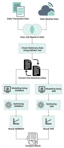
In this research, we are using transactions data from SME which took part in Food and Beverage (food and drink souvenirs) in small city Kudus, Central Java. our proposed methods can be seen as Figure 1.
From Figure 1, the detailed steps can be described as follows:
(1) We cleaning the transactions to obtain date and daily total transactions. The daily transaction data is based on showroom sales (physical store) and not considered the online sales (e-commerce or e-marketplace) due to we want to know the effect of weather in daily demand. The transactions data have several features such as: date (daily), and sales quantity (here, sales quantity is demand for that day). The daily transaction data is obtained from Januari 2023 to end of June 2023. The main reason for data collection to start in January 2023 is because that SME want to start fresh due to there is no COVID-19 anymore. Here, we only using one product which have best seller product called dodol (food made from sticky rice and brown sugar). The data can be seen at following Table 1.
(2) Then, we obtained daily weather data using BMKG (Indonesian Meteorological Agency). The obtained daily weather data are: dates, avg temperature and avg humidity.
(3) Finally, both daily transaction data and daily weather data are combined to become one dataset which can be seen at this Table 2.
Figure 1. Proposed methods
Table 1. Sales quantity data
|
Dates |
Sales Qty |
|
2023-01-09 |
14 |
|
2023-01-10 |
18 |
|
2023-01-11 |
16 |
|
2023-01-12 |
12 |
|
2023-01-13 |
19 |
|
… |
… |
|
2023-06-26 |
20 |
|
2023-06-27 |
17 |
|
2023-06-28 |
23 |
|
2023-06-29 |
26 |
|
2023-06-30 |
30 |
Table 2. Dataset contains sales qty, temp and humidity
| Dates | Sales Qty | Temp Avg | Humidity Avg |
| 2023/1/9 | 14 | 28 | 84 |
| 2023/1/10 | 18 | 27.9 | 85 |
| 2023/1/11 | 16 | 28.3 | 85 |
| 2023/1/12 | 12 | 28.7 | 80 |
| 2023/1/13 | 19 | 27.4 | 86 |
| … | … | … | ... |
| 2023/6/26 | 20 | 27.3 | 77 |
| 2023/6/27 | 17 | 28.6 | 79 |
| 2023/6/28 | 23 | 28.3 | 78 |
| 2023/6/29 | 26 | 28.9 | 80 |
| 2023/6/30 | 30 | 28.9 | 77 |
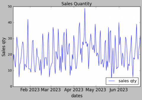
Figure 2. Plot for sales quantity by dates
Figure 3. Plot for temperature by dates
Figure 4. Plot for humidity by dates
Table 3. SARIMAX parameters value
|
Parameter |
Definition |
Range |
|
$p$ |
The number of lag observations included in the model |
[0,1,2,3,4] |
|
$d$ |
The degree of differencing |
[0,1] |
|
$q$ |
The size of the moving average window |
[0,1,2,3,4] |
|
$P$ |
It is similar to $p$ but applies to the seasonal component. |
[0,1,2,3,4] |
|
$D$ |
The number of times the seasonal observations are differenced to achieve stationarity. |
[0,1] |
|
$Q$ |
the size of the seasonal moving average window |
[0,1,2,3,4] |
|
$s$ |
the number of time steps in a single seasonal period (here, we take weekly) |
7 |
(4) For the dataset, we convert date into datetime format. Then, we plot the data as following Figures 2-4.
From the Figure 2, we can see that the daily demand has up and down.
From the Figure 3, we can also see that the temperature has up and downs. Here, the temperature tends to increase due the location has dry season when the dataset is collected.
From the Figure 4, we can also see that the humidity has tendency get low value due to dry season.
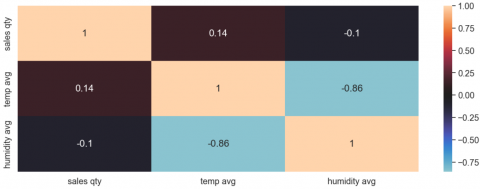
(1) After dataset is obtained, we check for correlation using pearson correlation test.
From Figure 5, we can see that temp avg have weak positive relationship with sales qty where the correlation coefficient of 0.15 suggests that there is a positive tendency: as one variable increases, the other variable tends to increase slightly as well. However, the relationship is not significant, and other factors are likely influencing the variability in the data. Then, the humidity avg have weak negative relationship with sales qty where a correlation coefficient of -0.11 that as one variable increases, the other variable tends to decrease slightly, and vice versa. The relationship, however, is not strong. Finally, humidity avg and temp avg obtained correlation coefficient of -0.86 which be interpreted as a clear inverse association between the variables. From here, we decided to use sales qty, temp avg and humidity avg as features.
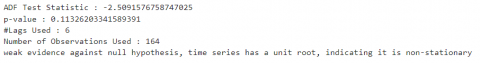
(2) Then, we are using adfuller test for stationary test. For this test, sales qty is used as target. Then, humidity avg and temp avg is used as exogeneous data.
From Figure 6, we found out that the data is non stationary. Thus, changing from non-stationary to stationary needs to be done. In here, differencing is embedded as value that are search for the optimum value in time series algorithm that we used.
(3) We are using two methods to compare, which methods is suitable for our dataset in daily demand prediction using sales quantity and weather data (temperature and humidity). Thus, here we are using SARIMAX and VAR.
(4) Here, the training data consist of date from 2023-01-09 to 2023-06-01 (total 142 rows). Then, for the testing data, it consists of date from 2023-06-01 to 2023-06-30 (total 30 rows).
(5) We are optimizing SARIMAX to obtain optimum value for $(p, d, q)$ and $(P, D, Q, s)$. Here, the parameter which considered in Table 3.
(1) We also optimizing VAR to obtain optimum value for the order with differencing value is set to 1.
(2) Finally, we compute the evaluation data from both SARIMAX and VAR with MSE, MAE and RMSE.
Figure 5. Pearson correlation value for dataset
Figure 6. Adfuller test result
The optimal results for SARIMX can be seen in Tables 4 and 5 as follows:
Table 4. SARIMAX model parameter
|
Model Number |
$d$ |
$D$ |
$p$ |
$q$ |
$P$ |
$Q$ |
|
1 |
0 |
0 |
0 |
0 |
2 |
2 |
|
2 |
0 |
1 |
0 |
0 |
2 |
2 |
|
3 |
1 |
0 |
2 |
3 |
2 |
2 |
|
4 |
1 |
1 |
2 |
3 |
2 |
2 |
The Table 2 contains information about the parameters used and put into model. Thus, the model Number is used as reference to Table 3 as follows:
Table 5. SARIMAX measurement results
|
Model Number |
AIC |
MSE |
MAE |
RMSE |
|
1 |
1106.74 |
73.582 |
7.344 |
8.578 |
|
2 |
1069.31 |
82.866 |
7.717 |
9.103 |
|
3 |
1102.41 |
75.711 |
7.481 |
8.701 |
|
4 |
1070.11 |
80.393 |
7.513 |
8.966 |
From Table 5 above, we chose the lowest AIC (1069.31) model number 2 where the d is 0, D is 1, p is 0, q is 0, P is 2, and Q is 2. Another lowest AIC is model number 4 (1070.11 and obtain better AIC, MSE, MAE and RMSE than before) where d is 1, D is 1, p is 2, q is 3, P is 2 and Q is 2. Although both is not gaining better measurement (MSE, MAE or RMSE) with other model, our primary goal is to understand the underlying patterns in the data, which AIC might be a more appropriate metric.
Thus, rather chose the lowest AIC, we took equilibrium (two lowest value and compare the MSE, MAE, RMSE), we can conclude that our dataset with (d=1, D=1, p=2, q=3, P=2, Q=2) needs differencing (d) and seasonal differencing (D) to become stationary (d), it needs 2 past observations (p), size of the moving average window is set to 2 which signifies the number of lagged forecast errors in the prediction equation (q), seasonal lag order is set to 2 (P), and size of the seasonal moving average window is set to 2.
For VAR, the VAR order can be seen as follows:
Table 6. VAR order selection (*highlights the minimum)
|
|
AIC |
BIC |
FPE |
HQIC |
|
0 |
6.954 |
7.020 |
1047 |
6.981 |
|
1 |
6.507 |
6.770* |
669.7 |
6.614 |
|
2 |
6.340 |
6.801 |
566.8 |
6.527 |
|
3 |
6.357 |
7.016 |
577.1 |
6.625 |
|
4 |
6.298 |
7.154 |
544.8 |
6.646 |
|
5 |
6.106 |
7.160 |
450.3 |
6.534 |
|
6 |
5.852 |
7.103 |
350.2 |
6.361* |
|
7 |
5.870 |
7.318 |
357.5 |
6.458 |
|
8 |
5.844* |
7.490 |
350.1* |
6.513 |
|
9 |
5.863 |
7.706 |
358.8 |
6.612 |
|
10 |
5.960 |
8.001 |
398.3 |
6.789 |
From Table 6 above, the lag number value for AIC, BIC FPE and HQIC is different. Thus, here we want to know, which order is better for our case (the sales qty is taken for best measurement).
Table 7. VAR measurement results
|
Order |
AIC |
MSE |
MAE |
RMSE |
|
8 (regarding AIC and PFE) |
2028.83 |
584.23 |
21.96 |
24.17 |
|
2 (regarding BIC) |
2093.93 |
548.20 |
21.93 |
23.41 |
|
6 (regarding HQIC) |
2030.47 |
571.13 |
22.06 |
23.89 |
Thus, from Table 7 above, we can conclude that the lag order chosen is 8 due to lowest AIC.
Finally, we compare SARIMAX with VAR to obtain the conclusion which one is better and presented in Table 8.
Table 8. Comparison measurement results
|
Model |
AIC |
MSE |
MAE |
RMSE |
|
SARIMAX (d=1, D=1, p=2, q=3, P=2, Q=2) |
1070.11 |
80.393 |
7.513 |
8.966 |
|
VAR (order 8) |
2028.835 |
584.233 |
21.966 |
24.171 |
From Table 8, we can conclude that SARIMAX is suitable for demand prediction regarding temp avg and humidity avg due to have lowest value in all measurements.
Daily Sales quantity and daily weather data (temp avg and humidity avg) can be used together with SARIMAX (d=1, D=1, p=2, q=3, P=2, Q=2, s=7) for Demand prediction with AIC 1070.11, MSE 80.393, MAE 7.513 and RMSE 8.966 rather than VAR (order 8) with AIC 2028.835, MSE 584.233, MAE 21.966 and RMSE 24.171.
As we know that the correlation between weather and sales have weak correlations, but with growing data, the weather data can be used for features as exogenous in SARIMAX algorithm.
In next research, we will observe the other features to obtain more optimum AIC, such as inflation, daily oil prices, etc and high spikes in holiday season.
We sincerely express our gratitude to the Directorate General of Higher Education, Research, and Technology, Ministry of Education, Culture, Research, and Technology of the Republic of Indonesia for funding a portion of this project through the Kedaireka Program. This is related to the grant contract document entitled "Implementation of Supply Chain Management System for MSMEs in the Food and Beverage Souvenir Sector, A Case Study in Central Java" with contract number 4501/F.9.02/UDN-01/IV/2023.
[1] Natariasari, R., Hariyani, E. (2023). Factors that influence taxpayer compliance with information knowledge technology as a moderating variable. Indonesian Journal of Economics, Social, and Humanities, 5(1): 21-33. https://doi.org/10.31258/ijesh.5.1.21-33
[2] Suryani, T., Fauzi, A.A., Sheng, M.L., Nurhadi, M. (2022). Developing and testing a measurement scale for SMEs’ website quality (SMEs-WebQ): Evidence from Indonesia. Electronic Commerce Research, 1-32. https://doi.org/10.1007/s10660-022-09536-w
[3] Herlinawati, A.E., Machmud, A., Suryana, S. (2020). Analysis of small medium enterprise business performance in Indonesia. In Advances in Business, Management and Entrepreneurship, CRC Press, pp. 905-907. https://doi.org/10.1201/9780429295348-191
[4] Do, H.H. (2021). The government supporting policy for sustainable development of small and medium industrial enterprises in Vietnam. Journal of Business Administration Research, 4(2): 1-10. https://doi.org/10.30564/jbar.v4i2.2938
[5] Sunuantari, M., Zarkasi, I.R., Gunawan, I., Farhan, R.M. (2021). R-TIK digital literacy towards Indonesian MSMEs (UMKM) digital energy of Asia. Komunikator, 13(2): 175-187. https://doi.org/10.18196/jkm.12380
[6] Hamburg, I. (2021). Impact of COVID-19 on SMEs and the role of digitalization. Advances in Research, 22(3): 10-17. https://doi.org/10.9734/air/2021/v22i330300
[7] Kolková, A., Ključnikov, A. (2022). Demand forecasting: AI-based, statistical and hybrid models vs practice-based models - The case of SMEs and large enterprises. Economics & Sociology, 15(4): 39-62. https://doi.org/10.14254/2071-789x.2022/15-4/2
[8] Chowdhury, M.T., Sarkar, A., Paul, S.K., Moktadir, M.A. (2022). A case study on strategies to deal with the impacts of COVID-19 pandemic in the food and beverage industry. Operations Management Research, 15(1): 166-178. https://doi.org/10.1007/s12063-020-00166-9
[9] Telukdarie, A., Munsamy, M., Mohlala, P. (2020). Analysis of the Impact of COVID-19 on the Food and Beverages Manufacturing Sector. Sustainability, 12(22): 9331. https://doi.org/10.3390/su12229331
[10] Zhang, G., Wang, T. (2022). Financial budgets of technology-based SMEs from the perspective of sustainability and big data. Frontiers in Public Health, 10: 861074. https://doi.org/10.3389/fpubh.2022.861074
[11] Hallak, R., Onur, I., Lee, C. (2022). Consumer demand for healthy beverages in the hospitality industry: Examining willingness to pay a premium, and barriers to purchase. Plos One, 17(5): e0267726. https://doi.org/10.1371/journal.pone.0267726
[12] Sah, S., Surendiran, B., Dhanalakshmi, R., Yamin, M. (2023). Covid-19 cases prediction using SARIMAX Model by tuning hyperparameter through grid search cross-validation approach. Expert Systems, 40(5): e13086. https://doi.org/10.1111/exsy.13086
[13] Andrianajaina, T., Razafimahefa, D.T., Rakotoarijaina, R., Haba, C.G. (2022). Grid search for SARIMAX parameters for photovoltaic time series modeling. Global Journal of Energy Technology Research Updates, 9: 87-96. https://doi.org/10.15377/2409-5818.2022.09.7
[14] Vaibhav, K., Saurabh, V., Mrunmayee, G., Atharva, C., Sandip, H. (2023). Electricity demand forecasting using time series analysis. International Research Journal of Modernization in Engineering Technology and Science, 1196-1215. https://doi.org/10.56726/irjmets35708
[15] Manigandan, P., Alam, M.S., Alharthi, M., Khan, U., Alagirisamy, K., Pachiyappan, D., Rehman, A. (2021). Forecasting natural gas production and consumption in United States-Evidence from SARIMA and SARIMAX models. Energies, 14(19): 6021. https://doi.org/10.3390/en14196021
[16] Fokker, E.S., Koch, T., van Leeuwen, M., Dugundji, E.R. (2022). Short-term forecasting of off-street parking occupancy. Transportation Research Record, 2676(1): 637-654. https://doi.org/10.1177/03611981211036373
[17] He, J., Wei, X., Yin, W., Wang, Y., Qian, Q., Sun, H., Xu, Y., Magalhaes, R.J.S., Guo, Y., Zhang, W. (2022). Forecasting scrub typhus cases in eight high-risk counties in China: Evaluation of time-series model performance. Frontiers in Environmental Science, 9: 783864. https://doi.org/10.3389/fenvs.2021.783864
[18] Balli, H.O., Tsui, W.H.K., Balli, F. (2019). Modelling the volatility of international visitor arrivals to New Zealand. Journal of Air Transport Management, 75: 204-214. https://doi.org/10.1016/j.jairtraman.2018.10.002
[19] Ampountolas, A. (2019). Forecasting hotel demand uncertainty using time series Bayesian VAR models. Tourism Economics, 25(5): 734-756. https://doi.org/10.1177/1354816618801741
[20] Ibrahim, A., Kashef, R., Li, M., Valencia, E., Huang, E. (2020). Bitcoin network mechanics: Forecasting the btc closing price using vector auto-regression models based on endogenous and exogenous feature variables. Journal of Risk and Financial Management, 13(9): 189. https://doi.org/10.3390/jrfm13090189
[21] Shah, I., Iftikhar, H., Ali, S., Wang, D. (2019). Short-term electricity demand forecasting using components estimation technique. Energies, 12(13): 2532. https://doi.org/10.3390/en12132532
[22] Benbekhti, S.E., Boulila, H., Bouteldja, A. (2021). Islamic finance, small and medium enterprises and job creation in turkey: An empirical evidence (2009-2017). International Journal of Islamic Economics and Finance (IJIEF), 4(SI): 41-62. https://doi.org/10.18196/ijief.v4i0.10490
[23] Xiao, S. (2020). Tax cuts and fee reductions and labor demand of SMEs. Financial Forum, 9(1): 1-5. https://doi.org/10.18282/ff.v9i1.800
[24] Oh, J., Ha, K.J., Jo, Y.H. (2021). New normal weather breaks a traditional clothing retail calendar. Preprint. https://doi.org/10.21203/rs.3.rs-213444/v1
[25] Silva, J.C., Figueiredo, M.C., Braga, A.C. (2019). Demand forecasting: A case study in the food Industry. Computational Science and Its Applications-ICCSA 2019. ICCSA 2019. Lecture Notes in Computer Science, Springer, Cham, 11621. https://doi.org/10.1007/978-3-030-24302-9_5
[26] Guinoubi, S., Hani, Y., Elmhamedi, A. (2021). Demand forecast; A case study in the agri-food sector: Cold. IFAC-PapersOnLine, 54(1): 993-998. https://doi.org/10.1016/j.ifacol.2021.08.191
[27] Du, M., Zhu, H., Yin, X., Ke, T., Gu, Y., Li, S., Li, Y., Zheng, G. (2022). Exploration of influenza incidence prediction model based on meteorological factors in Lanzhou, China, 2014–2017. Plos One, 17(12): e0277045. https://doi.org/10.1371/journal.pone.0277045
[28] Alharbi, F.R., Csala, D. (2022). A seasonal autoregressive integrated moving average with exogenous factors (SARIMAX) forecasting model-based time series approach. Inventions, 7(4): 94. https://doi.org/10.3390/inventions7040094
[29] Ma, J., Jia, Y., Lv, B. (2023). A hybrid forecasting model for monthly electricity consumption combining prophet and SARIMAX models. In Third International Conference on Advanced Algorithms and Neural Networks (AANN 2023), 12791: 626-631. https://doi.org/10.1117/12.3005085
[30] Chen, Y., Leng, K., Lu, Y., Wen, L., Qi, Y., Gao, W., Chen, H., Bai, L., An, X., Sun, B., Wang, P., Dong, J. (2020). Epidemiological features and time-series analysis of influenza incidence in urban and rural areas of Shenyang, China, 2010–2018. Epidemiology & Infection, 148: e29. https://doi.org/10.1017/S0950268820000151
[31] Kumari, S., Singh, S.K. (2023). Machine learning-based time series models for effective CO2 emission prediction in India. Environmental Science and Pollution Research, 30(55): 116601-116616. https://doi.org/10.1007/s11356-022-21723-8
[32] Suotsalo, K., Xu, Y., Corander, J., Pensar, J. (2021). High-dimensional structure learning of sparse vector autoregressive models using fractional marginal pseudo-likelihood. Statistics and Computing, 31: 1-18. https://doi.org/10.1007/s11222-021-10049-z