Gladys R. Velasco Chasipanta![]() | Nadia N. Sánchez-Pozo*
| Nadia N. Sánchez-Pozo*![]()
© 2024 The authors. This article is published by IIETA and is licensed under the CC BY 4.0 license (http://creativecommons.org/licenses/by/4.0/).
OPEN ACCESS
Forecasting exchange rates is a complex problem due to the inherent volatility and complex dynamics of exchange rates. Traditional forecasting models such as ARIMA often cannot capture these complexities especially for long-term forecasts. The objective of this study is to develop an accurate forecasting model for long-term exchange rates. A data set of euro-dollar exchange rates from 2017 to 2022 was used for the present analysis. ARIMA and MLP models were developed and their performances were compared; the optimized MLP model equipped with 11 input neurons derived from significant lags achieved a scaled mean absolute error (MASE) of 0.75 on the test data while the MLP model significantly outperformed the ARIMA model, demonstrating its ability to capture underlying patterns and trends in the exchange rate data. The optimized MLP model also provided a 365-day forecast for 2023 exchange rates. The results of this study suggest that MLP models are a promising tool for long-term forecasting of exchange rates. Their ability to capture complex nonlinear relationships and adapt to changing market conditions makes them well suited for this challenging task.
exchange rates, time series forecasting, ARIMA, neural network, MLP multilayer perceptron, accuracy, scaled mean absolute error (MASE), long-term prediction
The foreign exchange market is one of the largest and most dynamic financial environments in the world with a vast and constantly evolving environment due to the large volume of transactions reaching trillions of dollars daily, with the presence of constant flows of economic, political and social factors creating an environment of immense volatility and uncertainty, with this dynamic landscape, the ability to accurately predict price movements and discern underlying trends is critical to making successful trading decisions, which is a challenge for foreign exchange traders. Existing forecasting methods often struggle to capture the complex dynamics and non-linear relationships inherent in the euro-dollar foreign exchange market, limiting their ability to provide accurate long-term forecasts. Time series analysis is a classic technique used to analyze time series data and predict future trends with models such as ARIMA (Autoregressive Integrated Moving Average) [1] and modern techniques such as Machine Learning (ML) being used to understand market trends and improve forecast accuracy being a potential to refine the accuracy and reliability of forecasts in financial markets.
Previous studies highlighted "the effectiveness of time series analysis for understanding market properties and accurate and reliable forecasts" [2]. Moving averages "use past errors to predict future observations of currency prices" [3], ARIMA models, "incorporate AR, MA and I components, are used for financial time series modeling" [4]; currently MLP techniques have demonstrated the potential to refine the accuracy and reliability of forecasts in financial markets. However, despite advances, a crucial gap persists in existing forecasting methods as they often struggle to capture the complex dynamics and nonlinear relationships inherent in the Euro-dollar foreign exchange market, limiting their ability to provide accurate long-term forecasts.
In response to these challenges and gaps this study aims to develop a more accurate forecasting model for long-term exchange rates and minimize the existing gap by developing and evaluating two time series analysis models, in particular by integrating established techniques such as ARIMA with advanced machine learning models such as multilayer perceptron (MLP), this research strives to provide a more accurate and reliable forecast of exchange rate movements over extended periods of time.
1.1 Related works
In the study of Chang Rojas et al. [5], the focus was on developing forecast models to predict cargo throughput at the Port of Callao between 2019 and 2023. Utilizing SARIMAX time series models with exogenous inputs representing throughput and cargo of three port terminals (APMTC, DPWC, and TC), the results project a total cargo of 17 million tons and 3.4 million TEUs by 2023, opening investment opportunities for APMTC and DPWC due to the anticipated growth.
In the study of Sezer et al. [6], the article provides a comprehensive review on the use of deep learning (DL) for financial time series forecasting. The result is that DL models have significantly outperformed traditional methods. One study found that an LSTM model outperformed an ARIMA model in forecasting stock prices.
Mora Adan et al. [7] compared statistical models for predicting the profitability of Colombian financial institutions. GARCH and EGARCH outperform a dynamic polynomial model for all three entities, indicating that classical models are more suitable for forecasting financial stock profitability than dynamic polynomial models.
Argotty-Erazo et al. [8] developed a methodology for predicting the short-term directional movement of the euro-dollar exchange rate. The introduced Linear Classifier Configuration (LCC) methodology outperforms other sophisticated approaches, achieving an out-of-sample classification accuracy of 98.77%. LCC focuses on market inflection points and multidimensional differences between uptrends and downtrends.
Akhtar et al. [9] presented a stock prediction algorithm based on a support vector machine model, demonstrating an overall accuracy of 80.3%, surpassing existing methods.
In the study of Fischer and Krauss [10], LSTM networks are implemented to predict out-of-sample directional movements of S&P 500 index stocks from 1992 to 2015. The networks exhibit a daily return of 0.46% and a Sharpe ratio of 5.8 before transaction costs, proving LSTM networks suitable for financial time series forecasting.
Navia-Rodríguez et al. [11] aims to expose techniques, trends, and data used for algorithmic trading of financial assets. Machine learning, metaheuristics, neural networks, and fuzzy logic are identified as techniques reporting the best results.
In the study of Jagait et al. [12], propose an online adaptive ensemble learning approach, combining an online adaptive recurrent neural network (RNN) with an ARIMA model. The results show improved accuracy, with the proposed approach achieving a 30% forecast error reduction compared to the online adaptive RNN alone.
Roldan Martinez [13] compared the performance of the Black-Scholes model and the Heston model, concluding that the Heston model provides a better fit for short-term forecasts, while the Black-Scholes model excels in long-term forecasts.
In the study of Yu et al. [14] proposed a hybrid forecasting model for financial time series data, combining the Empirical Wavelet Transform (EWT), an improved Artificial Bee Colony (ABC) algorithm, an Extreme Learning Machine (ELM) neural network, and ARIMA. The hybrid model effectively removes data noise, corrects outliers, and coordinates linear and nonlinear patterns.
In the study of Abdoli [15], proposed an accurate forecasting model for the Tehran Stock Exchange (TSE), comparing LSTM and ARIMA. The LSTM model outperforms ARIMA in terms of prediction accuracy, especially in the short term.
Vo and Ślepaczuk [16], compared the performance of ARIMA and ARIMA-GARCH models for forecasting S&P500 returns. The main results indicate that ARIMA-GARCH hybrid models outperform ARIMA and a Buy & Hold strategy in the long run.
In the publication of Figal [17], fundamental analysis techniques are combined with signal extraction using a correlation matrix to analyze the relationships between variables and primary fundamental data in the foreign exchange market (FOREX) with the EUR/USD pair.
In the article of Siami-Namini and Namin [18], compared the forecasting performance of deep learning-based algorithms (LSTM) with traditional algorithms (ARIMA) for time series data, with LSTM models significantly outperforming ARIMA models.
In the study of Kobiela et al. [19], compared the performance of ARIMA and LSTM models for predicting daily and monthly average prices of NASDAQ-listed companies. For NASDAQ stocks with a single characteristic (historical price) and longer horizons, ARIMA is found to be a better choice than LSTM.
Peng et al. [20] develop a high-frequency prediction method for the cryptocurrency market. They propose a new attention-based CNN-LSTM model for multiple cryptocurrencies (ACLMC). it allows taking advantage of correlations between frequencies and coins to improve prediction accuracy.
In the study of Idrees et al. [21], an ARIMA model is used to forecast stock prices in the Indian stock market, with effective predictions observed based on various statistical measures.
Moews et al. [22] proposed a method for predicting directional trend changes in complex systems, utilizing lagged correlations and deep neural networks. The method, applied to historical stock data from 2011 to 2016, employs stepwise linear regressions as exponential smoothing.
The article of Meneses-Bautista and Alvarado [23] details the implementation of a multilayer perceptron (MLP) to forecast exchange rates in the foreign exchange market. The MLP, incorporating multiple exchange rates in the model, demonstrates an absolute error close to one cent, considered acceptable for forecasting applications.
Villamil Torres and Delgado Rivera [24] proposed an MLP to forecast exchange rates in the foreign exchange market for the euro/dollar pair. The MLP method, trained with historical data, employs multiple layers of neurons to capture nonlinear patterns and relationships in the data. The results show advanced prediction capabilities in capturing nonlinear patterns and adaptability to changes in the data over time.
In the present study, a model for forecasting the trend change in the foreign exchange market was obtained, for which the ARIMA model was selected as a representative of classical techniques and a set of neural network models under the backbone of multilayer perceptron (MLP), as a machine learning technique. For this study, the largest currency pair quoted in the market, which is the euro-dollar pair, was selected and historical data for the last 5 last years from March 2017 to December 2022 was used to train and test the models, the base was selected from the investing.com website for the choice of variables is determined based on general variables that apply in a technical analysis and relate to the price.
2.1 Data collection and preprocessing
Once selected the currency pair within the study period comprising 5.75 years, the historical data will serve to capture the cycles and trends of the market. The data was obtained from two sources of information, Yahoo Finance and Investing.com, which are platforms that provide technical information about the market, being selected the historical database of investing.com in a period from March 2017 to December 2022, these data refer to variables such as date, although time is not considered as a variable is important in the study, exchange rate, opening price, highest price, lowest price and closing price; Adjusted close, and volume, these variables consider the scenario within the technical environment in relation specifically to the price.
The study began by selecting the database with the most information on the variables under study. Next, a descriptive statistical analysis was performed, data processing techniques were applied, as well as data normalization techniques that allow the identification and elimination of atypical data. For data processing, Mahalanobis distances were used, based on the 7 numerical variables that made up the original database, considering a Chi-square distribution statistic for an interval of 99.9% of the distances, discriminating only 0.1% of the farthest distances. In this way, a cut-off score of 20.5150 was established by which a single atypical observation was detected, which was removed from the database, so that the final database consisted of 1304 observations.
2.2 Study variables
For this study, technical variables were selected that are generally considered for market analysis. These variables are presented in Table 1.
Table 1. Variables considered for market analysis
|
Variable |
Definition |
|
Exchange rate |
The currency of a country compared with another currency; in this case, the euro/dollar is considered. |
|
Historical exchange rate data |
Data set within a period that presents the exchange rate or currency. |
|
Opening price |
Price at the beginning of the day with which a currency pair begins to quote in the market. |
|
Highest price |
The highest value that a currency was quoted during the trading day. |
|
Lowest price |
The lowest value that a currency was quoted during the trading day. |
|
Closing price |
The last value that a currency was quoted in the market during the trading day. |
|
Time interval |
The temporality in which the analysis is carried out. This time interval can be annual, monthly, weekly, daily, hours, and minutes; this study applies a daily period. |
It should be emphasized that the date is not considered a study variable since it refers to time. However, the date of each observation is crucial for the analysis; For this study, a 5.75-year base of the euro-dollar pair was identified, starting from March 2017 to December 2022.
2.3 ARIMA models
Once the study variables were identified and the data processed, a time series analysis was performed using classical statistical techniques such as ARIMA. ARIMA models are commonly used in time series analysis to identify patterns in data, such as trends, seasonality, and residual components. For the application of the ARIMA model, the following process is required (Figure 1).
The ARIMA model is a time series analysis technique that uses past observations to predict future exchange rate values. The ARIMA equation is made up of three parts: the autoregressive (AR) model, the moving average (MA) model, and its respective integration (I). The general equation of an ARIMA (p, d, q) model is:
$\begin{gathered}y_t=c+\phi_1 \cdot y_{t-1}+\phi_2 \cdot y_{t-2}+\cdots+\phi_p \cdot y_{t-p} \\ +\theta_1 \cdot e_{t-1}+\theta_2 \cdot e_{t-2}+\cdots+\theta_q \cdot e_{t-q}+e_t\end{gathered}$ (1)
where, $y_t$ is the value of the variable observed in time $t, c$ is the model constant, $\phi_1, \phi_2, \ldots$, are the coefficients of the $\phi_p$ autoregressive model, which represent the effect of previous values of the time series on the current value, $\theta_1, \theta_2, \ldots, \theta_q$ are the coefficients of the moving average model, which represent the effect of past errors on the current value, $e_t$ is the error with respect to the reference value over time $t, p$ is the order of the autoregressive model, $d$ is the degree of integration, that is, the number of times the time series must be differentiated to make it stationary, and $q$ is the order of the moving average model.
The ARIMA equation was used to model a time series and predict its future values. The model coefficients can be estimated from the historical data of the time series, and once determined, they can be used to make the prediction.
Figure 1. Protocol for obtaining the ARIMA forecast model
2.4 Neural networks forecasting
In forecasting, an alternative that has shown great potential, especially for complex databases, is using artificial neural networks as an assembly technique. Each artificial neuron in the network mimics the behavior of a biological neuron, and its activation is based on a combination of input signals and a set of assigned weights. The combination of input signals must exceed a specific threshold for the neuron to fire and transmit a signal.
Several activation functions are available; however, in this work, the ReLU function is used for the hidden and output layers since a regression-type numerical output is expected. The input layer allows the network to enter any input variables without an activation function. Then, connections with assigned weights are established through the learning process so that different combinations of inputs can activate neurons in the hidden and output layers. This process allows each neuron or combination of neurons to learn nonlinear behaviors from the data. The propagation of signals in each layer of the neural network can be calculated using the expression:
$\begin{gathered}X_j=W_{i j} \cdot I \\ \mathcal{O}_j=\operatorname{activation}\left(X_j\right) .\end{gathered}$ (2)
where, $X_j$ is the matrix of resulting signals for a layer $j$ of the neural network, $W_{i j}$ corresponds to the matrix of weights of the existing links between a layer $j$ and its previous layer $i . I$ is the input signal matrix, and $\mathcal{O}_j$ represents the output signal matrix of each neural network layer after applying the activation function. Next, to enable the learning of a neural network, it is necessary to evaluate the error in each neuron of the final layer by comparing the obtained value with the expected value for each observation. This discrepancy is calculated using the formula $e_{o u t_k}=t_k-\sigma_k$. Subsequently, the error is propagated throughout the entire neural network, following the links where each output originated to allow the weight update. This process is carried out using the expression:
$\xi_i=W_{i j}^T \cdot \xi_j$ (3)
where, $\xi_i$, corresponds to the matrix of errors that will be back-propagated to the previous layer of the neural network, while $\xi_i$ refers to the errors that come from the next layer. Once the error backpropagation has occurred, the updated weights allow the neural network to retain information from previous examples and acquire new information from new observations. Gradient descent is one of the most widely used methods to achieve the objective of adjusting the weights of the neural network, which was formulated as follows:
$\begin{gathered}\frac{\partial \xi}{\partial W_{j k}}=\frac{\partial \sum_n\left(t_n-\sigma_n\right)}{\partial W_{j k}}=\frac{\partial \xi}{\partial \mathcal{O}_k} \cdot \frac{\partial \mathcal{O}_k}{\partial W_{j k}} =-2\left(t_n-\sigma_n\right) \cdot \frac{\partial \mathcal{O}_k}{\partial W_{j k}} \\ \frac{\partial \xi}{\partial W_{j k}}=-2\left(t_n-\sigma_n\right) \cdot \frac{\partial}{\partial W_{j k}} \text { activation }\left(\sum_j W_{j k} \cdot \mathcal{O}_j\right), W_{j k}^{(r+1)}=W_{j k}^{(r)}-\alpha \frac{\partial \xi}{\partial W_{j k}}\end{gathered}$ (4)
where, $W_{j k}^{(r+1)}$ corresponds to each new updated weight for a link $j_k$, which is updated from the previous parameter above $W_{j k}^{(r)}$, and the gradient $\partial \xi / \partial W_{j k}$ that provides a certain amount of newly learned information, which is moderated by the hyper-parameter learning-rate $\alpha$ [25, 26].
2.5 Precision metrics
The metrics that are typically used to determine forecast accuracy in time series are: mean square error (MSE), root mean square error (RMSE), mean absolute error (MAE), mean absolute percentage error (MAPE), and mean absolute scaled error (MASE); whose formulations are presented in Eqs (5-9):
$M S E=\frac{1}{n} \sum_{t=1}^{t=n}\left(y^{\prime}-y\right)^2,$ (5)
$R M S E=\sqrt{\frac{1}{n} \sum_{t=1}^{t=n}\left(y^{\prime}-y\right)^2},$ (6)
$M A E=\frac{1}{n} \sum_{t=1}^{t=n}\left|y^{\prime}-y\right|,$ (7)
$M A P E=\frac{1}{n} \sum_{t=1}^{t=n}\left|\frac{y^{\prime}-y}{y}\right| \cdot 100 \%,$ (8)
$MASE =\frac{1}{k} \frac{\sum_{t=1}^{t=k}\left|y_t^{\prime}-y_t\right|}{\frac{1}{m} \sum_{t=m+1}^{t=n}\left|y_t-y_{t-m}\right|},$ (9)
where, $y^{\prime}$ represents the predicted value, $y$ represents the actual value for each observation, $t$ represents the position at which each observation was recorded, and $n$ represents the total number of observations that make up the time series. It should be noted that, as suggested by Makridakis et al. [27], MASE is one of the most appropriate metrics to evaluate the behavior of various forecast models. However, the five metrics were addressed in this study, and the best models were selected based on the complete set of metrics.
2.6 Parameter selection
The selection of specific inputs and lags for the MLP model was based on the following rationale:
The adjusted closing price variable is selected because it is a value that more accurately reflects the true value of a currency at a given point in time. This is because it takes into account factors that can affect the closing price, such as dividends, distributions and corporate adjustments and is therefore considered a key variable for accurate historical and long-term analysis as it eliminates distortions caused by external events. In addition, by providing a more accurate picture of the evolution of the currency value, the adjusted closing price provides a more solid basis for analysis and forecasting.
The selection process employed a data-driven approach to identify the most influential delays and configure the input layer accordingly. This ensures that the MLP model is provided with relevant information for accurate predictions.
The data were divided into two sets: training and test. This allows to evaluate the performance of the model on unseen data and to avoid overfitting.
The percentage split applied corresponds to 90% training and 10% testing. Splitting allows training the model on most of the data and evaluating its performance on the remaining unseen data. This provides information on how the model generalizes to new data and avoids overfitting to the training data alone.
"Lags of the time series, potentially together with lagged observations of explanatory variables, are used as inputs to the network" [28]. The lags were selected in relation to the variability of the data, at the same time when applying a random works it was not possible to visualize the lags in the ACF and PACF digraphs, since this visualization was not available, we proceeded to run the function sel. lag and det. season, which allows running several models that in this case 100 observations were made in order to identify the most influential values.
The database obtained through Investing.com for the euro-dollar pair was structured to run the analysis from March 2017 to December 2022. The Mahalanobis distance technique was employed for data treatment, based on the seven numerical variables that constituted the original database. This approach involved considering a chi-square distribution statistic for a 99.9% interval of the distances, thereby discriminating only the furthest 0.1% of the distances. Consequently, a cutoff score of 20.5150 was established. Through this method, a single atypical observation was detected and subsequently removed from the database. As a result, the final database comprised 1304 observations.
The data was structured as a time series using the statistical programming language R. In this way, the database comprised 1304 observations taken for each day in the analysis period, structured into seven variables considering the date on which the observation was recorded and the values: open, high, low, close, adjusted close, and volume.
Table 2. Variables considered in the database
|
Variable |
Min. |
1st q. |
Median |
Half |
3rd q. |
Max. |
Deviation Standard |
|
open |
0.960 |
1.107 |
1.140 |
1.136 |
1.180 |
1.250 |
0.06040 |
|
High |
0.970 |
1.110 |
1.140 |
1.139 |
1.180 |
1.260 |
0.05987 |
|
low |
0.950 |
1.100 |
1.130 |
1.133 |
1.180 |
1.250 |
0.06068 |
|
close |
0.960 |
1.110 |
1.140 |
1.136 |
1.180 |
1.250 |
0.06043 |
|
Adj.Close |
0.960 |
1.110 |
1.140 |
1.136 |
1.180 |
1.250 |
0.06043 |
Of these seven variables, this research focused on the adjusted close since this corresponds to the daily close of the euro-dollar pair after the adjustments applied for all the divisions and distributions of the applicable dividends. This value is adjusted using the appropriate division and dividend multipliers following the Center for Research in Securities Prices (CRSP) standards. For these reasons, the adjusted closing value Adj.Close was the most appropriate value to use in a foreign exchange market forecast analysis. The descriptive statistics of the variables that constituted the database are presented in Table 2.
3.1 Time series analysis
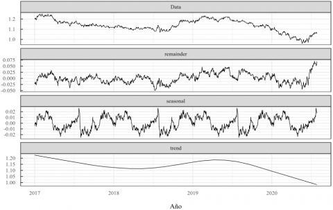
Next, a data visualization analysis was carried out to determine the type of time series the case study corresponds to. For this, a time series decomposition was carried out considering the components, seasonal, trend, and residuals. The results of this decomposition are presented in Figure 2.
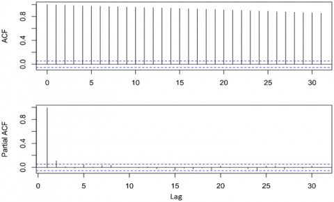
As can be seen in Figure 2, the time series has a considerable random behavior since, when performing the temporal decomposition on a weekly or monthly basis, its trend component presented an unpredictable behavior, even for an annual period with a frequency of 365, its trend component continued to present a pattern that was difficult to interpret. For these reasons, the Dickey-Fuller test was executed, and the ACF graphs (Autocorrelation Function) and PACF (Partial Autocorrelation Function), in order to identify the type of time series for this case study. The results of the Dickey-Fuller test and the ACF and PACF diagrams are presented in Table 3 and Figure 3.
Table 3. Dickey-Fuller test applied to the variable Adj.Close
|
Augmented Dickey-Fuller Test |
|||||
|
Dickey-Fuller |
-1.5486 |
lag order |
10 |
p-value |
0.7694 |
|
Alternative hypothesis: |
Stationary |
||||
Figure 2. Decomposition of the time series into its components: seasonal, trend, and residuals
Figure 3. ACF and PACF autocorrelation diagrams for the variable Adj.Close
As shown in Table 3, the Dickey-Fuller test did not reach the significance level of 0.05, where the configured null hypothesis was: "the time series is not seasonal." In this way, the null hypothesis could not be rejected, so the time series was not seasonal. In addition, in the Figure 3 ACF diagram, it can be observed that the autocorrelation of the time series fails to reach the level of significance (blue lines), even after a Lag of order 30. In addition, in the PACF diagram, it was possible to visualize that the time series could present a significant autocorrelation after a Lag of order one. However, due to the serious autocorrelation problems evidenced in the ACF, it was concluded that the time series corresponds to a Random Walk, categorized as a case similar to white noise. The Random Walk is a complex forecasting case, so it was decided to implement the classical ARIMA model and compare it with more robust models based on neural networks to identify the most appropriate for this problem.
3.2 ARIMA models
To successfully run the ARIMA model on a Random Walk, it is preferred to comply with the assumption of seasonality. For this reason, a MA (moving average) appropriate for the data series was selected, outliers were removed, and the time series was differentiated. The smoothed time series results for a weekly and monthly moving average (MA) are presented in Figure 4.
As seen in Figure 4, for the time series of this case study, it is possible to select a monthly moving average since it correctly smoothes the data series without losing too much information regarding the trend and seasonality of the series. In addition, a data treatment was executed to correct missing and atypical data problems, for which 36 observations were removed and imputed using the function tsclean. In this way, by applying a monthly moving average, data processing, and differentiation of order one of the time series, it was possible to obtain a data set that complies with the stationarity assumption for the euro-dollar pair. The results of the Dickey-Fuller test and the ACF and PACF graphs for this new data set are presented in Table 4 and Figure 5.
Figure 4. Smoothed time series for a daily (red), weekly (blue), and monthly (green) moving average
Figure 5. ACF and PACF autocorrelation diagrams for the variable Adj.Close after data treatment and order one differentiation
Figure 6. Residuals plot, ACF, and ACF autocorrelations for the ARIMA model fitted using the training data
As seen in Table 4, after treatment and differentiation of the data, the new numerical set complies with the Dickey-Fuller test. Similarly, the autocorrelation diagrams show that the autocorrelation quickly enters the significance zone, evidencing a Lag of order one in the partial autocorrelation diagram. In this way, with the new, improved numerical set, an ARIMA model was developed for the time series of the euro-dollar pair.
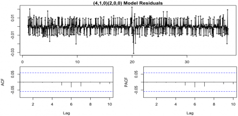
First, the data set was divided in a ratio of 6 to 1 , taking the data from March 2017 to December 2021 as training data, and the data from the last year 2022, was reserved as test data to validate the model. In this way, the appropriate ARIMA model for the data set was determined using the function auto. arima, under a seasonal configuration, considering the terms that produce trend drift (allow. drift =$T$ ) and the first order Lag identified in the autocorrelation diagrams. In this way, the model obtained by the library auto.arima and its residual diagram are presented in Table 5 and Figure 6.
$\begin{gathered}y_t=-0.174330 \cdot y_{t-1}-0.042586 \cdot y_{t-2}+0.009431 \\ \cdot y_{t-3}-0.067671 \cdot y_{t-4}-0.017949 \\ \cdot e_{t-1}-0.044088 \cdot e_{t-2}+e_t\end{gathered},$ (10)
Table 4. Dickey-Fuller test applied to the Adj.Close variable after data treatment and order one differentiation
|
Augmented Dickey-Fuller Test |
|||||
|
Dickey-Fuller |
-12.354 |
lag order |
10 |
p-value |
0.01 |
|
Alternative hypothesis: |
Stationary |
||||
Table 5. Results obtained by fitting the ARIMA model for the treated data
|
Output Model : ARIMA(4,1,0)(2,0,0) |
||||||
|
|
ar1 |
ar2 |
ar3 |
ar4 |
sar1 |
sar2 |
|
coeff. |
-0.1743 |
-0.0426 |
0.0094 |
-0.0677 |
-0.0179 |
-0.0441 |
|
HE |
0.0302 |
0.0307 |
0.0308 |
0.0304 |
0.0315 |
0.0319 |
|
$\sigma^2$ =3.475e-05: log likelihood=4070.54 AIC=-8127.08 AICc=-8126.98 BIC=-8092.09 |
||||||
Table 6. Performance metrics of the ARIMA model applied to unobserved test data
|
MSE |
RMSE |
MAE |
MAP |
MASE |
|
0.004758 |
0.068981 |
0.059429 |
0.057070 |
783.097245 |
Figure 7. Forecast results for the year 2022 using the ARIMA model
As shown in Figure 6, the model obtained has acceptable performance for the training data, and none of the observations considered for 10 Lags were outside the region of significance. Finally, using the ARIMA model obtained, the expected values for January to December 2022 that the ARIMA model did not observe during its training were forecast. These data were also compared with the real values for that period, and the performance metrics for the forecast model were obtained. The forecast results for the year 2022 are presented in Figure 7, and the performance metrics of the model are presented in Table 6.
As seen in Table 5, the ARIMA model did not have an appropriate performance for obtaining the forecast for 365 days since its performance metrics were found to have very high values and did not reach an acceptable value for the forecast model. In addition, several tests were performed with different custom ARIMA models; however, their results were similar to the model provided by the function auto. arima, therefore, it was concluded that the ARIMA model is not appropriate for this forecast case, especially for a large forecast horizon.
3.3 Multilayer perceptron
For the reasons stated above and because the ARIMA model could not reach optimal performance values, it was decided to implement a model based on neural networks using the $R$ library. This particular library nnfor was proposed in the beginning by Kourentzes et al. [28-30] and has been continually improved to date. This library includes numerous tools that facilitate the development of neural network models for forecasting in complex time series, especially through its functions $m l p$ (multilayer perceptron) and $e l m$ (extreme learning machines). The function was selected for this study $m l p$, because it has widely proven to be an excellent tool for forecasting complex non-seasonal time series, at the same time, artificial neural networks are able to capture the short- and long-term nonlinear components of a time series [31].
In this way, the neural network models were developed under the same protocol used in the ARIMA models, so again, all the observations from March 2017 to December 2021 were used as training data, and the data for the year 2022 were reserved for validation and verification of the performance of the model on unobserved data.
Next, the automatic detection module of the neural network configuration was executed to have a notion of the most appropriate type of topology for the neural network, in addition to the most influential Lags found in the time series, for this the $m l p$ function was run on the training data with the sel.lag and det.season parameters turned on and optimal neuron number detection for the hidden layer enabled. In this way, after 100 training stages and the verification of different intervals for Lags selection, it was obtained as a first approximation that the most influential Lags for the time series were found in locations 1, 2, 441, 442, 447, 448, 453, 534, 631, 746 and 764 , so one neuron was configured in the input layer to be trained to capture the behavior of the data each time the period described by each Lag interval. For this reason, the input laver of the MLP consisted of 11 neurons.
Next, we proceeded to verify the behavior of the neural networks for different numbers of neurons in the first hidden layer, covering a range from 5 to 22 neurons, which were trained during 33 training stages that correspond to triple the number of input variables, as suggested by Demuth et al. [25]. At the end of each processing stage, the forecast was executed for a horizon equivalent to the observations of the year 2022, and the predicted values were compared with the actual Adj.Close values allowed the estimation of the performance metrics of each model. The results for all the models evaluated for the first hidden layer of the MLP are presented in Table 7.
As can be seen in Table 6 and Figure 8, the configuration that presented the best performance in the forecast of the data for the data from the year 2022 that was not observed during training was the model of 17 neurons in the hidden layer, which reached a MASE of 3.073914, which is considerably lower than the MASE obtained using the ARIMA models. However, based on the recommendations of the study by Demuth et al. [25, 30], a MASE of 3.073914 is not acceptable for an appropriate forecast. For this reason, we proceeded to explore the alternatives and existing configurations for the second hidden layer of the MLP. Considering the first hidden layer comprised 17 neurons, the models were explored from half to twice as many neurons as the first layer (8 to 34 neurons). The results are presented in Table 8.
Table 7. Performance metrics of the neural network models tested for the first layer of the MLP using different numbers of neurons
|
Number of Neurons |
MSE |
RMSE |
MAE |
MAP |
MASE |
|
5 |
0.000556 |
0.023584 |
0.020708 |
0.001556 |
4.006042 |
|
6 |
0.000704 |
0.026531 |
0.022429 |
-0.000995 |
4.339158 |
|
7 |
0.000620 |
0.024891 |
0.020259 |
0.008999 |
3.919286 |
|
8 |
0.001069 |
0.032700 |
0.025928 |
0.011638 |
5.015885 |
|
9 |
0.000595 |
0.024392 |
0.018721 |
0.007474 |
3.621783 |
|
10 |
0.001423 |
0.037720 |
0.031613 |
0.012184 |
6.115839 |
|
11 |
0.003768 |
0.061387 |
0.049826 |
-0.025899 |
9.639311 |
|
12 |
0.000671 |
0.025911 |
0.021238 |
0.005612 |
4.108728 |
|
13 |
0.000703 |
0.026506 |
0.021163 |
0.010170 |
4.094089 |
|
14 |
0.000509 |
0.022553 |
0.017221 |
-0.013564 |
3.331593 |
|
15 |
0.001168 |
0.034170 |
0.027368 |
0.021765 |
5.294473 |
|
16 |
0.001496 |
0.038681 |
0.031143 |
-0.026564 |
6.024793 |
|
17 |
0.000403 |
0.020072 |
0.015889 |
-0.002453 |
3.073914 |
|
18 |
0.001150 |
0.033907 |
0.027462 |
0.017343 |
5.312720 |
|
19 |
0.001077 |
0.032819 |
0.023238 |
0.007198 |
4.495576 |
|
20 |
0.003165 |
0.056258 |
0.047502 |
0.045328 |
9.189631 |
|
21 |
0.001110 |
0.033310 |
0.024423 |
0.004359 |
4.724733 |
|
22 |
0.001890 |
0.043478 |
0.036476 |
0.034982 |
7.056665 |
Table 8. Performance metrics of the neural network models tested for the second layer of the MLP using different numbers of neurons
|
Number of Neurons |
MSE |
RMSE |
MAE |
MAP |
MASE |
|
8 |
0.001175 |
0.034276 |
0.027626 |
0.024285 |
5.344417 |
|
9 |
0.002114 |
0.045975 |
0.038219 |
0.036635 |
7.393788 |
|
10 |
0.001736 |
0.041667 |
0.033374 |
0.029106 |
6.456476 |
|
11 |
0.002404 |
0.049035 |
0.038745 |
0.033810 |
7.495575 |
|
12 |
0.004722 |
0.068719 |
0.057650 |
0.055911 |
11.152802 |
|
13 |
0.001079 |
0.032843 |
0.026040 |
0.021713 |
5.037697 |
|
14 |
0.001214 |
0.034842 |
0.027474 |
0.022086 |
5.315082 |
|
15 |
0.002276 |
0.047709 |
0.038535 |
0.034049 |
7.454931 |
|
16 |
0.001559 |
0.039488 |
0.030742 |
0.020485 |
5.947237 |
|
17 |
0.001419 |
0.037675 |
0.031860 |
0.001909 |
6.163533 |
|
18 |
0.001462 |
0.038238 |
0.029576 |
0.026942 |
5.721656 |
|
19 |
0.001413 |
0.037591 |
0.028433 |
0.023545 |
5.500672 |
|
20 |
0.000683 |
0.026137 |
0.021174 |
0.001573 |
4.096343 |
|
21 |
0.000621 |
0.024923 |
0.019167 |
0.008217 |
3.707934 |
|
22 |
0.002195 |
0.046856 |
0.041101 |
0.039325 |
7.951279 |
|
23 |
0.001381 |
0.037161 |
0.027478 |
0.012755 |
5.315751 |
|
24 |
0.001725 |
0.041528 |
0.032027 |
0.028891 |
6.195891 |
|
25 |
0.004169 |
0.064566 |
0.052248 |
0.049693 |
10.107697 |
|
26 |
0.002696 |
0.051922 |
0.042048 |
0.034458 |
8.134585 |
|
27 |
0.000236 |
0.008322 |
0.002238 |
0.002537 |
0.754487 |
|
28 |
0.003749 |
0.061229 |
0.048766 |
0.040080 |
9.434163 |
|
29 |
0.005216 |
0.072224 |
0.057017 |
0.054333 |
11.030310 |
|
30 |
0.000840 |
0.028991 |
0.022265 |
-0.011511 |
4.307374 |
|
31 |
0.001531 |
0.039123 |
0.032719 |
0.024447 |
6.329817 |
|
32 |
0.002205 |
0.046957 |
0.035940 |
0.034059 |
6.952953 |
|
33 |
0.002576 |
0.050754 |
0.043938 |
0.042893 |
8.500096 |
|
34 |
0.000972 |
0.031171 |
0.025233 |
0.021813 |
4.881605 |
As can be seen in Table 8 and Figure 9, the model that obtained the best performance in the metrics was the one with 27 neurons in the second hidden layer, which reached an MSE of 0.000236, RMSE of 0.008322, MAE of 0.002238, MAPE of 0.002537 and a MASE of 0.754487. In this way, it was possible to appreciate that the model reached excellent performance metrics that guarantee an excellent forecast. Especially the MASE reached a value lower than one, which according to the study by Kourentzes et al. [28], categorizes it as an excellent forecast model whose precision is similar to that observed in the previous time series period. Finally, the possibility of improving the neural network architecture by adding an additional hidden layer was explored. For this reason, 42 neural network models were redesigned and validated for configurations from 13 to 54 neurons in the third hidden layer. The results are presented in Table 9.
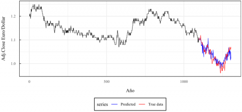
As seen in Table 9, adding a third layer in the neural network architecture presents overfitting problems in the model, which is evidenced by the fact that none of the models designed with three layers performed better than the best two-layer model selected in the previous stage. For this reason, the incorporation of additional hidden layers in the MLP was not continued, so the multilayer perceptron with 11 neurons in the input layer was selected as the best configuration (representing Lags of order 1, 2, 441, 442, 447, 448, 453, 534, 631, 746 and 764) and 17 and 27 neurons in its two hidden layers. This configuration had an excellent performance which is visible when forecasting the data for the year 2022 that were never observed during the training stage. The forecast results of the best proposed neural network model contrasted with the actual data of the time series for the year 2022 are presented in Figure 10.
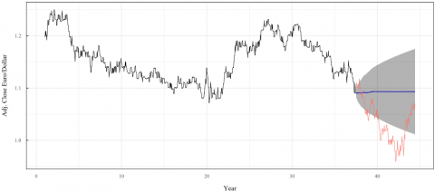
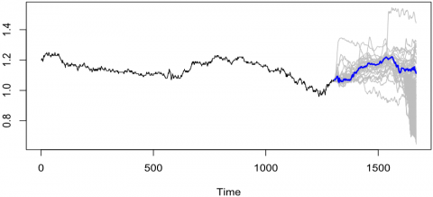
Finally, using the best MLP model obtained and validated on the test data, a daily forecast was obtained for 2023, from January to the end of June and was obtained covering a forecast horizon of 365 days. The parameters used were the same as the model that obtained the best MASE of 0.754487 for the neuron configuration (11,17,27,1). The results obtained with the neural network were compared with the real data that have elapsed until the end of June 2023 and the same metrics were obtained, reaching an MSE of 0.770410. The results are presented in Figure 11 and Table 10.
Table 9. Performance metrics of the neural network models tested for the third layer of the MLP using different numbers of neurons
|
Number of Neurons |
MSE |
RMSE |
MAE |
MAP |
MASE |
|
13 |
0.001594 |
0.039924 |
0.031185 |
0.027642 |
6.032958 |
|
14 |
0.004437 |
0.066612 |
0.056120 |
0.055067 |
10.856763 |
|
15 |
0.004508 |
0.067145 |
0.056170 |
0.054597 |
10.866537 |
|
16 |
0.001840 |
0.042890 |
0.034799 |
0.032098 |
6.732218 |
|
17 |
0.003551 |
0.059586 |
0.048981 |
0.046826 |
9.475774 |
|
18 |
0.004221 |
0.064967 |
0.054151 |
0.052332 |
10.476023 |
|
19 |
0.001961 |
0.044283 |
0.036510 |
0.034242 |
7.063242 |
|
20 |
0.002375 |
0.048733 |
0.039394 |
0.037992 |
7.620990 |
|
21 |
0.003345 |
0.057836 |
0.048824 |
0.046864 |
9.445429 |
|
22 |
0.003591 |
0.059928 |
0.046562 |
0.045236 |
9.007835 |
|
23 |
0.002347 |
0.048449 |
0.041027 |
0.039485 |
7.937028 |
|
24 |
0.003947 |
0.062822 |
0.054566 |
0.053129 |
10.556315 |
|
25 |
0.002957 |
0.054377 |
0.043565 |
0.040926 |
8.428045 |
|
26 |
0.003919 |
0.062605 |
0.053243 |
0.051987 |
10.300368 |
|
27 |
0.002284 |
0.047794 |
0.039097 |
0.036836 |
7.563631 |
|
28 |
0.006669 |
0.081664 |
0.068817 |
0.067490 |
13.313233 |
|
29 |
0.001559 |
0.039480 |
0.033420 |
0.030539 |
6.465278 |
|
30 |
0.004002 |
0.063260 |
0.053784 |
0.052116 |
10.404880 |
|
31 |
0.002737 |
0.052313 |
0.045114 |
0.043579 |
8.727639 |
|
32 |
0.004951 |
0.070365 |
0.059850 |
0.058582 |
11.578414 |
|
33 |
0.003562 |
0.059684 |
0.049484 |
0.047656 |
9.573101 |
|
34 |
0.003126 |
0.055907 |
0.048055 |
0.046562 |
9.296593 |
|
35 |
0.004187 |
0.064711 |
0.050026 |
0.048204 |
9.677987 |
|
36 |
0.004060 |
0.063716 |
0.052963 |
0.045057 |
10.246027 |
|
37 |
0.001294 |
0.035970 |
0.028544 |
0.026061 |
5.521983 |
|
38 |
0.002672 |
0.051689 |
0.042074 |
0.038781 |
8.139495 |
|
39 |
0.003825 |
0.061844 |
0.053865 |
0.052654 |
10.420667 |
|
40 |
0.001866 |
0.043200 |
0.033527 |
0.028120 |
6.485987 |
|
41 |
0.002843 |
0.053322 |
0.043706 |
0.038855 |
8.455307 |
|
42 |
0.005957 |
0.077183 |
0.062812 |
0.061405 |
12.151486 |
|
43 |
0.002918 |
0.054014 |
0.042167 |
0.034598 |
8.157486 |
|
44 |
0.001568 |
0.039601 |
0.031761 |
0.029720 |
6.144417 |
|
45 |
0.002108 |
0.045914 |
0.031808 |
0.016705 |
6.153585 |
|
46 |
0.004143 |
0.064367 |
0.053563 |
0.051711 |
10.362224 |
|
47 |
0.002222 |
0.047139 |
0.037434 |
0.035185 |
7.241957 |
|
48 |
0.004666 |
0.068311 |
0.056511 |
0.054910 |
10.932510 |
|
49 |
0.008829 |
0.093961 |
0.078519 |
0.077206 |
15.190192 |
|
50 |
0.004406 |
0.066375 |
0.052921 |
0.051096 |
10.237950 |
|
51 |
0.001900 |
0.043592 |
0.036464 |
0.030624 |
7.054319 |
|
52 |
0.003599 |
0.059990 |
0.050022 |
0.047846 |
9.677082 |
|
53 |
0.002008 |
0.044811 |
0.036082 |
0.033236 |
6.980333 |
|
54 |
0.002433 |
0.049329 |
0.040252 |
0.033579 |
7.787070 |
Figure 8. Architecture of the best configuration determined for the first hidden layer of the multilayer perceptron
Figure 9. Architecture of the best configuration determined for the second hidden layer of the multilayer perceptron
Figure 10. Forecast results obtained using the best MLP model for the data from the year 2022 that were not observed during the training process
Figure 11. Forecast results obtained using the best MLP model for the 365 days of the year 2023
Table 10. Forecast of adjusted closing values for each day of the year 2023
|
Date |
Adj.Close |
Date |
Adj.Close |
Date |
Adj.Close |
Date |
Adj.Close |
|
1/1/2023 |
1.069869 |
2/4/2023 |
1.096243 |
2/7/2023 |
1.167558 |
1/10/2023 |
1.207487 |
|
2/1/2023 |
1.068813 |
3/4/2023 |
1.095438 |
3/7/2023 |
1.170884 |
2/10/2023 |
1.199370 |
|
3/1/2023 |
1.064583 |
4/4/2023 |
1.094171 |
4/7/2023 |
1.169238 |
3/10/2023 |
1.195714 |
|
4/1/2023 |
1.065382 |
5/4/2023 |
1.094139 |
5/7/2023 |
1.168564 |
4/10/2023 |
1.192879 |
|
5/1/2023 |
1.065132 |
6/4/2023 |
1.093928 |
6/7/2023 |
1.171122 |
5/10/2023 |
1.183981 |
|
6/1/2023 |
1.067348 |
7/4/2023 |
1.092859 |
7/7/2023 |
1.171950 |
6/10/2023 |
1.183319 |
|
7/1/2023 |
1.069493 |
8/4/2023 |
1.095460 |
8/7/2023 |
1.172407 |
7/10/2023 |
1.169891 |
|
8/1/2023 |
1.073075 |
9/4/2023 |
1.095086 |
9/7/2023 |
1.171950 |
8/10/2023 |
1.165498 |
|
9/1/2023 |
1.076562 |
10/4/2023 |
1.098476 |
10/7/2023 |
1.173057 |
9/10/2023 |
1.167963 |
|
10/1/2023 |
1.076073 |
11/4/2023 |
1.097336 |
11/7/2023 |
1.170547 |
10/10/2023 |
1.164010 |
|
11/1/2023 |
1.079253 |
12/4/2023 |
1.099302 |
12/7/2023 |
1.171982 |
11/10/2023 |
1.163350 |
|
12/1/2023 |
1.082126 |
4/13/2023 |
1.099574 |
7/13/2023 |
1.169846 |
10/12/2023 |
1.163518 |
|
1/13/2023 |
1.081225 |
4/14/2023 |
1.101062 |
7/14/2023 |
1.170463 |
10/13/2023 |
1.158458 |
|
1/14/2023 |
1.071900 |
4/15/2023 |
1.102386 |
7/15/2023 |
1.175412 |
10/14/2023 |
1.156387 |
|
1/15/2023 |
1.071006 |
4/16/2023 |
1.100749 |
7/16/2023 |
1.176977 |
10/15/2023 |
1.152936 |
|
1/16/2023 |
1.068328 |
4/17/2023 |
1.102313 |
7/17/2023 |
1.178712 |
10/16/2023 |
1.150751 |
|
1/17/2023 |
1.067515 |
4/18/2023 |
1.107304 |
7/18/2023 |
1.178522 |
10/17/2023 |
1.143489 |
|
1/18/2023 |
1.067992 |
4/19/2023 |
1.109189 |
7/19/2023 |
1.180256 |
10/18/2023 |
1.142290 |
|
1/19/2023 |
1.066275 |
4/20/2023 |
1.109969 |
7/20/2023 |
1.180105 |
10/19/2023 |
1.136620 |
|
1/20/2023 |
1.061460 |
4/21/2023 |
1.110632 |
7/21/2023 |
1.182653 |
10/20/2023 |
1.134988 |
|
1/21/2023 |
1.061696 |
4/22/2023 |
1.111924 |
7/22/2023 |
1.180798 |
10/21/2023 |
1.134299 |
|
1/22/2023 |
1.060875 |
4/23/2023 |
1.112849 |
7/23/2023 |
1.185754 |
10/22/2023 |
1.138668 |
|
1/23/2023 |
1.057924 |
4/24/2023 |
1.110112 |
7/24/2023 |
1.184457 |
10/23/2023 |
1.136951 |
|
1/24/2023 |
1.056239 |
4/25/2023 |
1.111196 |
7/25/2023 |
1.187138 |
10/24/2023 |
1.141613 |
|
1/25/2023 |
1.056907 |
4/26/2023 |
1.113620 |
7/26/2023 |
1.188875 |
10/25/2023 |
1.144532 |
|
1/26/2023 |
1.058934 |
4/27/2023 |
1.117603 |
7/27/2023 |
1.191879 |
10/26/2023 |
1.146694 |
|
1/27/2023 |
1.065069 |
4/28/2023 |
1.118186 |
7/28/2023 |
1.192743 |
10/27/2023 |
1.153931 |
|
1/28/2023 |
1.064617 |
4/29/2023 |
1.119857 |
7/29/2023 |
1.190867 |
10/28/2023 |
1.152228 |
|
1/29/2023 |
1.063709 |
4/30/2023 |
1.121316 |
7/30/2023 |
1.192774 |
10/29/2023 |
1.151872 |
|
1/30/2023 |
1.063787 |
5/1/2023 |
1.125476 |
7/31/2023 |
1.189343 |
10/30/2023 |
1.151820 |
|
1/31/2023 |
1.061913 |
2/5/2023 |
1.124216 |
1/8/2023 |
1.188853 |
10/31/2023 |
1.152715 |
|
2/1/2023 |
1.059317 |
3/5/2023 |
1.120453 |
2/8/2023 |
1.191239 |
1/11/2023 |
1.154780 |
|
2/2/2023 |
1.061831 |
4/5/2023 |
1.123209 |
3/8/2023 |
1.191227 |
2/11/2023 |
1.155253 |
|
2/3/2023 |
1.062507 |
5/5/2023 |
1.127158 |
4/8/2023 |
1.190580 |
3/11/2023 |
1.155692 |
|
4/2/2023 |
1.063137 |
6/5/2023 |
1.126708 |
5/8/2023 |
1.189391 |
4/11/2023 |
1.153778 |
|
5/2/2023 |
1.063632 |
7/5/2023 |
1.129132 |
6/8/2023 |
1.190619 |
5/11/2023 |
1.149278 |
|
6/2/2023 |
1.060881 |
8/5/2023 |
1.133671 |
7/8/2023 |
1.190759 |
6/11/2023 |
1.143766 |
|
7/2/2023 |
1.059216 |
9/5/2023 |
1.134289 |
8/8/2023 |
1.192651 |
7/11/2023 |
1.138483 |
|
8/2/2023 |
1.063656 |
10/5/2023 |
1.131512 |
9/8/2023 |
1.195455 |
8/11/2023 |
1.140317 |
|
9/2/2023 |
1.064205 |
11/5/2023 |
1.130983 |
10/8/2023 |
1.197440 |
9/11/2023 |
1.135885 |
|
10/2/2023 |
1.066733 |
12/5/2023 |
1.134490 |
11/8/2023 |
1.197895 |
11/10/2023 |
1.133087 |
|
11/2/2023 |
1.066414 |
5/13/2023 |
1.136598 |
12/8/2023 |
1.200568 |
11/11/2023 |
1.127930 |
|
2/12/2023 |
1.068771 |
5/14/2023 |
1.137807 |
8/13/2023 |
1.201913 |
11/12/2023 |
1.122696 |
|
2/13/2023 |
1.066852 |
5/15/2023 |
1.136903 |
8/14/2023 |
1.203665 |
11/13/2023 |
1.120289 |
|
2/14/2023 |
1.065296 |
5/16/2023 |
1.139067 |
8/15/2023 |
1.206716 |
11/14/2023 |
1.113966 |
|
2/15/2023 |
1.065099 |
5/17/2023 |
1.137042 |
8/16/2023 |
1.209659 |
11/15/2023 |
1.113098 |
|
2/16/2023 |
1.062374 |
5/18/2023 |
1.139352 |
8/17/2023 |
1.209233 |
11/16/2023 |
1.118609 |
|
2/17/2023 |
1.062343 |
5/19/2023 |
1.137919 |
8/18/2023 |
1.212740 |
11/17/2023 |
1.120192 |
|
2/18/2023 |
1.061103 |
5/20/2023 |
1.135952 |
8/19/2023 |
1.209894 |
11/18/2023 |
1.117599 |
|
2/19/2023 |
1.065055 |
5/21/2023 |
1.137027 |
8/20/2023 |
1.209202 |
11/19/2023 |
1.116253 |
|
2/20/2023 |
1.063869 |
5/22/2023 |
1.133620 |
8/21/2023 |
1.213161 |
11/20/2023 |
1.120292 |
|
2/21/2023 |
1.068383 |
5/23/2023 |
1.136074 |
8/22/2023 |
1.219860 |
11/21/2023 |
1.125994 |
|
2/22/2023 |
1.068517 |
5/24/2023 |
1.135341 |
8/23/2023 |
1.227204 |
11/22/2023 |
1.135434 |
|
2/23/2023 |
1.067605 |
5/25/2023 |
1.135973 |
8/24/2023 |
1.229240 |
11/23/2023 |
1.124932 |
|
2/24/2023 |
1.069276 |
5/26/2023 |
1.136478 |
8/25/2023 |
1.228803 |
11/24/2023 |
1.122034 |
|
2/25/2023 |
1.069414 |
5/27/2023 |
1.138735 |
8/26/2023 |
1.226694 |
11/25/2023 |
1.119809 |
|
2/26/2023 |
1.066438 |
5/28/2023 |
1.138530 |
8/27/2023 |
1.217214 |
11/26/2023 |
1.141510 |
|
2/27/2023 |
1.065983 |
5/29/2023 |
1.141712 |
8/28/2023 |
1.213014 |
11/27/2023 |
1.117629 |
|
2/28/2023 |
1.066723 |
5/30/2023 |
1.141798 |
8/29/2023 |
1.208671 |
11/28/2023 |
1.119955 |
|
3/1/2023 |
1.070094 |
5/31/2023 |
1.144493 |
8/30/2023 |
1.213066 |
11/29/2023 |
1.115652 |
|
2/3/2023 |
1.068250 |
1/6/2023 |
1.147026 |
8/31/2023 |
1.210198 |
11/30/2023 |
1.118723 |
|
3/3/2023 |
1.067410 |
2/6/2023 |
1.145895 |
1/9/2023 |
1.210936 |
1/12/2023 |
1.119502 |
|
4/3/2023 |
1.068961 |
3/6/2023 |
1.148401 |
2/9/2023 |
1.209759 |
2/12/2023 |
1.123430 |
|
5/3/2023 |
1.070197 |
4/6/2023 |
1.152577 |
3/9/2023 |
1.208163 |
3/12/2023 |
1.115799 |
|
6/3/2023 |
1.072149 |
5/6/2023 |
1.154678 |
4/9/2023 |
1.207097 |
4/12/2023 |
1.117801 |
|
7/3/2023 |
1.071924 |
6/6/2023 |
1.154367 |
5/9/2023 |
1.211321 |
5/12/2023 |
1.112432 |
|
8/3/2023 |
1.071066 |
7/6/2023 |
1.154674 |
6/9/2023 |
1.210223 |
6/12/2023 |
1.125670 |
|
9/3/2023 |
1.071527 |
8/6/2023 |
1.155760 |
7/9/2023 |
1.212250 |
7/12/2023 |
1.127729 |
|
10/3/2023 |
1.069370 |
9/6/2023 |
1.158330 |
8/9/2023 |
1.213636 |
8/12/2023 |
1.133516 |
|
11/3/2023 |
1.069197 |
10/6/2023 |
1.157513 |
9/9/2023 |
1.217562 |
9/12/2023 |
1.132011 |
|
12/3/2023 |
1.076167 |
11/6/2023 |
1.158715 |
10/9/2023 |
1.222032 |
10/12/2023 |
1.135831 |
|
3/13/2023 |
1.075720 |
12/6/2023 |
1.159807 |
11/9/2023 |
1.223017 |
11/12/2023 |
1.136262 |
|
3/14/2023 |
1.074130 |
6/13/2023 |
1.162973 |
12/9/2023 |
1.224871 |
12/12/2023 |
1.137048 |
|
3/15/2023 |
1.073307 |
6/14/2023 |
1.163732 |
9/13/2023 |
1.225798 |
12/13/2023 |
1.135627 |
|
3/16/2023 |
1.075041 |
6/15/2023 |
1.167470 |
9/14/2023 |
1.226021 |
12/14/2023 |
1.131302 |
|
3/17/2023 |
1.083772 |
6/16/2023 |
1.168983 |
9/15/2023 |
1.224375 |
12/15/2023 |
1.137471 |
|
3/18/2023 |
1.089486 |
6/17/2023 |
1.169985 |
9/16/2023 |
1.223920 |
12/16/2023 |
1.140902 |
|
3/19/2023 |
1.094676 |
6/18/2023 |
1.170461 |
9/17/2023 |
1.221552 |
12/17/2023 |
1.141348 |
|
3/20/2023 |
1.101203 |
6/19/2023 |
1.170718 |
9/18/2023 |
1.219886 |
12/18/2023 |
1.143559 |
|
3/21/2023 |
1.106690 |
6/20/2023 |
1.169468 |
9/19/2023 |
1.218594 |
12/19/2023 |
1.151159 |
|
3/22/2023 |
1.114564 |
6/21/2023 |
1.169153 |
9/20/2023 |
1.216317 |
12/20/2023 |
1.151391 |
|
3/23/2023 |
1.102486 |
6/22/2023 |
1.173301 |
9/21/2023 |
1.217376 |
12/21/2023 |
1.143828 |
|
3/24/2023 |
1.091442 |
6/23/2023 |
1.172563 |
9/22/2023 |
1.217908 |
12/22/2023 |
1.137523 |
|
3/25/2023 |
1.086885 |
6/24/2023 |
1.174147 |
9/23/2023 |
1.210661 |
12/23/2023 |
1.142344 |
|
3/26/2023 |
1.087748 |
6/25/2023 |
1.172530 |
9/24/2023 |
1.208321 |
12/24/2023 |
1.146069 |
|
3/27/2023 |
1.089396 |
6/26/2023 |
1.173569 |
9/25/2023 |
1.203784 |
12/25/2023 |
1.133315 |
|
3/28/2023 |
1.093189 |
6/27/2023 |
1.174913 |
9/26/2023 |
1.202675 |
12/26/2023 |
1.135375 |
|
3/29/2023 |
1.097086 |
6/28/2023 |
1.174449 |
9/27/2023 |
1.202996 |
12/27/2023 |
1.131574 |
|
3/30/2023 |
1.102948 |
6/29/2023 |
1.171950 |
9/28/2023 |
1.206607 |
12/28/2023 |
1.130300 |
|
3/31/2023 |
1.100734 |
6/30/2023 |
1.170912 |
9/29/2023 |
1.208558 |
12/29/2023 |
1.135980 |
|
4/1/2023 |
1.096537 |
1/7/2023 |
1.168098 |
9/30/2023 |
1.207390 |
12/30/2023 |
1.134823 |
The MLP model outperforms the ARIMA model for long-term forecasts and the classical ARIMA model could not provide a sufficiently accurate forecast for a 365-day forecast horizon. In contrast, the MLP model achieved a MASE of 0.754487, which is considered an excellent value for long-term forecasts. This suggests that the MLP model is better suited for forecasting complex data and longer time horizons. Similar to what was reported in empirical data [18], in this study, it was possible to observe that the classical ARIMA method was not able to deliver a forecast that had a sufficient level of accuracy relative to the LSTM. Similar to what is proposed in studies specialized in the foreign exchange market [23, 24], it focuses its work with the ML method. The MLP multilayer perceptron and was implemented using the R package, which was much more robust when dealing with complex data such as Random Walk, addressed in this study. As seen in the results section, it was necessary to implement many neural network models to discover the appropriate topology for the neural network in each of its layers.
The MASE metric is the best for assessing long-term forecast accuracy compared to other metrics such as MSE, RMSE, MAE and MAPE; MASE is more sensitive to small variations and improvements in model performance, which makes it a better option for assessing long-term forecast accuracy; in a similar study [8], mentions that it is desirable to pay attention to the metrics. From the metrics used in this analysis, similar to that reported by Basu et al. [32], it can be observed that the metric that best reflects the accuracy of the executed forecast is the MASE since this metric is at an adequate scale that allows considering even small variations and improvements in the performance of a model to adequately visualize it at a scale greater or less than one. On the other hand, the MSE, RMSE, MAE and MAP metrics retrieve values at a small scale, making it difficult to read these subtle differences and select the best model.
MLP outperforms ARIMA for non-seasonal data, while ARIMA models can perform well for short-term forecasts and seasonal data, they are less accurate for long-term forecasts with non-seasonal data. The MLP model, on the other hand, is highly effective for long-term forecasts regardless of seasonality. The results observed in the Table 11 show a clear superiority of the MLP model (11,17,27,1), which achieved a MASE of 0.754487, considered an acceptable value, and categorizes it as an excellent model, in contrast to the ARIMA models whose best representative achieved an excessively high MASE of 783.097245. This clearly indicates that, although the ARIMA model applied to forex time series forecasts performs well in short time intervals and seasonal series, its accuracy is relatively poor when working with long forecast horizons, especially with non-seasonal data. For its part, the MLP is a model that has been widely spread nowadays [28, 29, 33]; and its high forecasting ability is evident when dealing with long forecast horizons, being able to execute an excellent task even for the 365-day horizon presented in this case study.
Table 11. Comparative metrics ARIMA and MLP model
|
Model |
Mse |
Rmse |
Mae |
Map |
MASE |
|
ARIMA |
0.004758 |
0.068981 |
0.059429 |
0.057070 |
783.097245 |
|
MLP-17 |
0.000403 |
0.020072 |
0.015889 |
-0.002453 |
3.073914 |
|
MLP-27 |
0.000236 |
0.008322 |
0.002238 |
0.002537 |
0.754487 |
Machine learning methods (MLP) outperform ARIMA models for forecasting trend changes in the foreign exchange market, especially for long forecast horizons and non-seasonal data; the foreign exchange market is a non-seasonal market, so MLP models would fit the best option for forecasting in this market.
In a daily seasonality and 365 range, the MLP model becomes an attractive technique for long-term forecasting with non-seasonal data based on the optimal configurations that best fit the data set variable; The optical configuration of the MLP for this type of forecasting consists of 11 neurons in the input layer, 17 neurons in the hidden layer 1 and 27 neurons in the hidden layer 2.
The MASE metric is the most suitable for selecting the best forecasting method for the change of trend in the foreign exchange market, since it presents an adequate scale to visualize the subtle but essential improvements in the configuration of the different forecasting models. In addition, through multiple training stages, it was possible to obtain a sufficiently robust MLP model that reached a value of 0. 754487 for the mean absolute scaled error (MASE), which guarantees a forecast with a confidence level similar to the data corresponding to the previous year, through which the forecast for the exchange market corresponding to the year 2023 is made, which is presented as a result of the present research. Continuing with the above, it is recommended to move forward with analyses that support the findings [28]; as well as with modern models that allow achieving much more accurate forecasts and the introduction of modern models such as LSTM [8] for long-term forecasts and with non-seasonal data.
[1] Cortes Chala, O., Wilches Moreno, C.E. (2022). Modelo de precio de las acciones del índice Dow Jones por medio de series de tiempo en modelo ARIMA y aplicación de modelo red neuronal. Especialización en Estadística Aplicada. https://repository.libertadores.edu.co/bitstream/handle/11371/4728/Cortes_Wilches_2022.pdf?sequence=1&isAllowed=y
[2] Ayala Castrejón, R.F., Bucio Pacheco, C. (2020). Modelo ARIMA aplicado al tipo de cambio peso-dólar en el periodo 2016-2017 mediante ventanas temporales deslizantes. Revista Mexicana de Economía y Finanzas, 15(3): 331-354. https://doi.org/10.21919/remef.v15i3.466
[3] Broncano, R.E. (2022). Aplicación de técnicas de machine learning para la predicción de los precios de la acción APPLE. Revista de Investigación de Sistemas e Informática, 15(1): 13-22. https://doi.org/10.15381/risi.v15i1.23737
[4] Montoya Zapata, C., Corredor Roa, C.A. (2022). Aplicación de modelos de deep learning y machine learning para el pronóstico de la serie de tiempo del par de divisas Euro-Dólar. Especializaciones de la Facultad de Ingeniería, pp. 2003-2005.
[5] Chang Rojas, V.A. (2019). Un análisis de series de tiempo mediante modelos SARIMAX para la proyección de demanda de carga en el puerto del Callao. Revista de Análisis Económico y Financiero, 1(3): 15-31. https://www.aulavirtualusmp.pe/ojs/index.php/raef/article/view/1694
[6] Sezer, O.B., Gudelek, M.U., Ozbayoglu, A.M. (2020). Financial time series forecasting with deep learning: A systematic literature review: 2005-2019. Applied Soft Computing, 90: 106181. https://doi.org/10.1016/j.asoc.2020.106181
[7] Mora Adan, P.A. (2020). Comparación de modelos clásicos en series de tiempo y modelos bayesianos para pronosticar tres acciones colombianas en el último año. Universidad Santo Tomás, pp. 1-20. https://repository.usta.edu.co/bitstream/handle/11634/31657/2020paulamora.pdf?sequence=1&isAllowed=y
[8] Argotty-Erazo, M., Blázquez-Zaballos, A., Argoty-Eraso, C.A., Lorente-Leyva, L.L., Sánchez-Pozo, N.N., Peluffo-Ordóñez, D.H. (2023). A novel linear-model-based methodology for predicting the directional movement of the euro-dollar exchange rate. IEEE Access, 11: 67249-67284. https://doi.org/10.1109/ACCESS.2023.3285082
[9] Akhtar, M.M., Zamani, A.S., Khan, S., Shatat, A.S.A., Dilshad, S., Samdani, F. (2022). Stock market prediction based on statistical data using machine learning algorithms. Journal of King Saud University-Science, 34(4): 101940. https://doi.org/10.1016/j.jksus.2022.101940
[10] Fischer, T., Krauss, C. (2018). Deep learning with long short-term memory networks for financial market predictions. European Journal of Operational Research, 270(2): 654-669. https://doi.org/10.1016/j.ejor.2017.11.054
[11] Navia-Rodríguez, J.R., Cobos-Lozada, C.A., Mendoza-Becerra, M.E. (2020). Trading algorítmico para la predicción de series de tiempo financieras: Una revisión sistemática. Revista Ibérica de Sistemas e Tecnologias de Informação, E38: 337-357.
[12] Jagait, R.K., Fekri, M.N., Grolinger, K., Mir, S. (2021). Load forecasting under concept drift: Online ensemble learning with recurrent neural network and ARIMA. IEEE Access, 9: 98992-99008. https://doi.org/10.1109/ACCESS.2021.3095420
[13] Roldan Martinez, L.C. (2018). Forecasting latin-american currency exchange using models with static and stochastic volatility. Ingeniería, 23(2): 166-189. https://doi.org/10.14483/23448393.12726
[14] Yu, H., Ming, L.J., Sumei, R., Shuping, Z. (2020). A hybrid model for financial time series forecasting-integration of EWT, ARIMA with the improved ABC optimized ELM. IEEE Access, 8: 84501-84518. https://doi.org/10.1109/ACCESS.2020.2987547
[15] Abdoli, G. (2020). Comparing the prediction accuracy of LSTM and ARIMA models for time-series with permanent fluctuation. Periódico do Núcleo de Estudos e Pesquisas sobre Gênero e DireitovCentro de Ciências Jurídicas-Universidade Federal da Paraíba, 9(2): 314-339. https://doi.org/10.22478/ufpb.2179-7137.2020v9n2.50782
[16] Vo, N., Ślepaczuk, R. (2022). Applying hybrid ARIMA-SGARCH in algorithmic investment strategies on S&P500 Index. Entropy, 24(2): 158. https://doi.org/10.3390/e24020158
[17] Figal, A.G. (2021). Pronóstico de la tasa de cambio euro-dólar. Diagnóstico de técnicas predictivas. Universidad de La Habana, 12(3). https://doi.org/10.33936/eca_sinergia.v12i3.3024
[18] Siami-Namini, S., Namin, A.S. (2018). Forecasting economics and financial time series: ARIMA vs. LSTM. arXiv Preprint arXiv: 1803.06386. https://doi.org/10.48550/arXiv.1803.06386
[19] Kobiela, D., Krefta, D., Król, W., Weichbroth, P. (2022). ARIMA vs LSTM on NASDAQ stock exchange data. Procedia Computer Science, 207: 3836-3845. https://doi.org/10.1016/j.procs.2022.09.445
[20] Peng, P., Chen, Y., Lin, W., Wang, J.Z. (2024). Attention-based CNN-LSTM for high-frequency multiple cryptocurrency trend prediction. Expert Systems with Applications, 237: 121520. https://doi.org/10.1016/j.eswa.2023.121520
[21] Idrees, S.M., Alam, M.A., Agarwal, P. (2019). A prediction approach for stock market volatility based on time series data. IEEE Access, 7: 17287-17298. https://doi.org/10.1109/ACCESS.2019.2895252
[22] Moews, B., Herrmann, J.M., Ibikunle, G. (2019). Lagged correlation-based deep learning for directional trend change prediction in financial time series. Expert Systems with Applications, 120: 197-206. https://doi.org/10.1016/j.eswa.2018.11.027
[23] Meneses-Bautista, F.D., Alvarado, M. (2017). Pronóstico del tipo de cambio USD/MXN con redes neuronales de retropropagación. Research in Computing Science, 139: 97-110. https://doi.org/10.13053/rcs-139-1-8
[24] Villamil Torres, J.A., Delgado Rivera, J.A. (2007). Training a multilayer neural network for the Euro-dollar (EUR/USD) exchange rate. Ingeniería e Investigación, 27(3): 106-117.
[25] Demuth, H.B., Beale, M.H., De Jess, O., Hagan, M.T. (2014). Neural network design. Martin Hagan. https://hagan.okstate.edu/NNDesign.pdf
[26] Weidman, S. (2019). Deep learning from scratch: Building with python from first principles. O'Reilly Media.
[27] Makridakis, S., Spiliotis, E., Assimakopoulos, V. (2018). Statistical and machine learning forecasting methods: Concerns and ways forward. PloS One, 13(3): e0194889. https://doi.org/10.1371/journal.pone.0194889
[28] Kourentzes, N., Barrow, D.K., Crone, S.F. (2014). Neural network ensemble operators for time series forecasting. Expert Systems with Applications, 41(9): 4235-4244. https://doi.org/10.1016/j.eswa.2013.12.011
[29] Crone, S.F., Kourentzes, N. (2010). Feature selection for time series prediction-A combined filter and wrapper approach for neural networks. Neurocomputing, 73(10-12): 1923-1936. https://doi.org/10.1016/j.neucom.2010.01.017
[30] Ord, K., Fildes, R.A., Kourentzes, N. (2017). Principles of business forecasting. Wessex Press Publishing Co.
[31] Parot, A., Michell, K., Kristjanpoller, W.D. (2019). Using artificial neural networks to forecast exchange rate, including VAR‐VECM residual analysis and prediction linear combination. Intelligent Systems in Accounting, Finance and Management, 26(1): 3-15. https://doi.org/10.1002/isaf.1440
[32] Basu, T., Menzer, O., Ward, J., SenGupta, I. (2022). A novel implementation of siamese type neural networks in predicting rare fluctuations in financial time series. Risks, 10(2): 39. https://doi.org/10.3390/risks10020039
[33] Kourentzes, N., Petropoulos, F., Trapero, J.R. (2014). Improving forecasting by estimating time series structural components across multiple frequencies. International Journal of Forecasting, 30(2): 291-302. https://doi.org/10.1016/j.ijforecast.2013.09.006