Vijay Kumar Kangala*![]() | Rajeswara Rao Ramisetty
| Rajeswara Rao Ramisetty![]()
© 2023 IIETA. This article is published by IIETA and is licensed under the CC BY 4.0 license (http://creativecommons.org/licenses/by/4.0/).
OPEN ACCESS
Speaker diarization, the task of ascertaining speaker homogeneity within a collection of audio recordings featuring multiple speakers, is crucial for answering queries such as "who spoke when". Diverse speaker recordings, encompassing meetings, reality shows, and news broadcasts, typically populate the speaker diarization database. Traditional methods primarily rely on clustering speaker embeddings, yet these approaches often fail to minimize diarization errors effectively and struggle to accurately account for speaker overlaps. Addressing these limitations, we propose a robust model leveraging the Fractional Ebola Optimization Search Algorithm (FEOSA) for speaker segmentation and diarization. This model represents an amalgamation of the Fractional Calculus (FC) concept and the Ebola Optimization Search Algorithm (EOSA), thereby enhancing the efficacy of the diarization process. The diarization task is executed employing an entropy weighted power k-means algorithm, with weights updated via the proposed FEOSA. The proposed FEOSA demonstrated superior testing accuracy, reaching a maximum of 0.913, and significantly reduced diarization errors to a minimum of 0.566. Further, False Discovery Rate (FDR), False Negative Rate (FNR) and False Positive Rate (FPR) were recorded at 0.257, 0.128, and 0.104 respectively, underscoring the effectiveness of the proposed model in enhancing speaker diarization.
speech signal, speaker diarization, Fractional Calculus (FC), deep learning, Ebola Optimization Search Algorithm (EOSA)
The proliferation of large-scale audio data, including voice mails, broadcasts, meetings, and a myriad of spoken files, has led to a significant reduction in cost and an increase in access to computational power, storage capacity, and bandwidth [1]. This surge necessitates the development of efficient automatic human language technologies to facilitate effective indexing, searching, and retrieval of these rich informational sources. A key element in this process is speaker indexing, where labels corresponding to speaker identities are assigned to different segments of an audio file [2].
An audio file comprises various sources, requiring an indexing process that categorizes the signal into speech and non-speech signals, the latter of which includes silence, music, and noise [3]. With the exponential growth of recorded speech, encompassing audio broadcasts, voice messages, and television, speaker diarization has emerged as a significant task. The objective of this technique is to partition the speech signal and isolate signals from the same speaker, essentially answering "who spoke what and when" [3].
Speaker diarization has found practical applications in reports, broadcast news, interviews, debates, and more. It is also commonly employed in tasks such as speaker detection, broadcast meetings, speaker recognition, video segmentation, and multimedia summarization [4, 5]. Diarization tasks, particularly audio-based diarization, present a series of challenges due to overlapping speech utterances from different speakers, background noises, reverberations, and short utterances [6, 7].
Traditionally, speaker diarization models have relied on partitioning the audio stream into speaker-homogenous parts. However, these models are often compromised by environmental factors like noise and reverberation [8]. Speaker diarization typically involves two primary phases [9]. The initial phase is segmentation, where audio features are refined and a speaker change identification is performed. The second phase is clustering, where segments from the same speaker are grouped together under the same label [10]. Yet, the accurate representation of speech partitions and maintaining the purity of each cluster continue to pose significant challenges [10].
Various clustering techniques have been employed for speaker diarization, including K-means, spectral clustering (SC), agglomerative hierarchical clustering (AHC) [11], and affinity propagation [12]. Among these, bottom-up clustering has been the most prevalent approach, starting with individual segments and continuously combining adjacent groups until a specific criterion is met. Conversely, top-down clustering begins by treating the entire audio as a single entity and progressively divides it into subclusters. Both strategies, while effective, are continuous processes and face the limitation of error propagation [3].
Recent years have seen the rise of neural network embedding as a standard technique for diarization tasks. However, most neural network-based speaker embedding extractors are trained on large datasets that may not always be readily accessible [13]. Training neural networks using raw waveforms is a recent trend that discards the feature extraction pipeline and yields better results for tasks like speech recognition [14, 15], speaker verification [16], and emotional identification [17, 18]. Despite these advances, constructing an end-to-end objective function for speaker diarization issues that is invariant with respect to speaker order and number remains a challenging task [12].
This article's primary goal is to develop an effective framework for speaker segmentation and diarization using the proposed Fractional Ebola Optimization Search Algorithm (FEOSA). A set of features, including Mel Frequency Cepstral Coefficients (MFCC), Linear Prediction Cepstral Coefficients (LPCC), Line Spectral Frequency (LSF), Zero Crossing Rate, Spectral Skewness, Spectral Rolloff, Logarithmic Band Power, Spectral Spread, Fast Fourier Transform (FFT), Spectral Centroid, and Power Spectral Density, are extracted from audio input samples for further processing. Subsequently, speech activity is identified to distinguish speech signals from non-speech ones. Speaker segmentation is then carried out based on speaker change detection, where constant thresholds are computed using the proposed FEOSA, a novel technique developed by integrating the concept of Fractional Calculus (FC) with the Ebola Optimization Search Algorithm (EOSA). The final step involves speaker diarization or clustering, where the same speech signal is grouped into one category using an entropy-weighting power k-means algorithm. The weight update is heavily reliant on the newly developed FEOSA.
The primary innovation of this research is the introduction of the Fractional Ebola Optimization Search Algorithm (FEOSA) for speaker segmentation and diarization. The proposed model is premised on a novel algorithm, FEOSA, designed to conduct speaker segmentation based on speaker change detection. Critical to this process is the computation of constant thresholds, which is executed using the newly proposed FEOSA. Moreover, the task of clustering is accomplished via an entropy-weighting power k-means approach, where the weight is updated based on the same FEOSA.
This research paper is organized as follows: Section 2 provides a comprehensive review of eight recently published classical techniques, delineating their respective advantages and limitations. Section 3 articulates the workings of the proposed FEOSA for speaker diarization. Section 4 presents the results and a comparative analysis of the new approach against the existing methods. Section 5 concludes the study, offering insights into potential future research directions.
This section provides the underpinning for the study by reviewing eight current publications on speaker diarization. The strengths and limitations of each study serve as the impetus for the development of a more effective model for speaker segmentation and diarization.
The pertinent studies are summarized as follows:
VijayKumar and Rao [3] developed a bottom-up speaker clustering technique enabled by active learning, aiming to improve diarization performance with minimal human intervention. Their approach comprised two phases-exploratory clustering and constrained clustering-wherein an active learning algorithm was utilized to generate precise speaker models and facilitate audio grouping. Despite achieving a significant reduction in the diarization error rate (DER) using a limited number of queries, the method showed insufficiencies in addressing human errors.
Karim et al. [10] proposed a model for speaker clustering in speaker diarization using the differential evolution (DE) and K-means algorithm. The model employed two norms—trace within criterion (TRW) and variance ratio criterion (VRC)-as grouping validity indices. Despite the superior results compared to non-hybrid algorithms, the model was not tested with various clustering validity criteria such as Davies and Bouldin (DB) index and Clustering Separation criterion (CS).
Ahmad et al. [8] introduced a Long Short-Term Memory (LSTM)-based speech enhancement block for the speech diarization process, fine-tuned on an artificial dataset with over 100 types of noises. While it successfully reduced speech distortion, the complexity of the system increased considerably.
Pal et al. [19] developed the meta-ClusterGAN (MCGAN) under the meta-learning framework for speaker diarization. Despite the method's high performance on five diverse datasets, it has not been tested with various meta-learning algorithms. In a separate study, Pal et al. [20] presented a deep latent space clustering model for speaker diarization using GAN backprojection with the assistance of an encoder network. The model outperformed existing x-vector-based diarization models, but the utilization of spectrograms as GAN input rather than pre-trained embeddings was suggested for future work. Ahmad et al. [6] developed a multimodal speaker diarization system that utilized an audio-visual synchronization system for diarization. While it successfully created speaker-specific clusters, it failed to yield satisfactory results when multiple speakers spoke simultaneously. Dubey et al. [17] implemented a SincNet in a vanilla transfer learning (VTL) setup for speaker diarization, achieving remarkable results even when trained on sparse data.
Finally, Wang et al. [12] devised Graph Neural Networks (GNNs) for speaker diarization, refining speaker embeddings using structural information and mapping them into a new embedding space. Despite the model's superior performance on both simulated and original meetings, the challenges of audio-based diarization remained, including overlapping speech from different speakers, distortions, low utterances, and reverberations.
The following encapsulates the contributions and shortcomings of each study:
In the study by VijayKumar and Rao [3], an expected speaker-error-based segment selection approach was employed, demonstrating superior efficacy over random segment selection. However, this strategy failed to accommodate the study of human errors, leading to potential shortcomings in system performance.
In the work of Karim et al. [10], a hybrid DE algorithm was designed, outperforming non-hybrid algorithms concerning indexation outcomes. Yet, it was not validated using various clustering validity criteria, such as the Davies and Bouldin (DB) index and Clustering Separation criterion (CS), thus constraining the generalizability of the results.
Ahmad et al. [8] devised a Long Short-Term Memory (LSTM)-based speech enhancement model, proving to be an optimal choice for denoising both Additive White Gaussian Noise (AWGN) and environmental noises. Despite reducing the system error, the enhancement led to an increase in the complexity of the system, posing challenges in practical implementation.
In a separate contribution, Pal et al. [19] utilized pre-trained placings as input, although a direct examination of speech spectrograms could have been more valuable. Additionally, the method was not tested with various meta-learning algorithms, limiting its robustness.
Finally, the diarization process often faces considerable challenges when only unimodal information is available. Audio-based diarization, in particular, is fraught with complexities due to overlapping speech from different speakers, distortions, low utterances, and reverberations.
The core intention of this research is speaker segmentation and speaker diarization using proposed FEOSA, which is the integration of FC [21] and EOSA [22]. Initially, the input audio sample taken from Telugu dataset specified in the study [23] is allowed for the process of feature extraction. After the process of extracting required features, Speech activity identifications carried out for clearly identifying the signal from non-speech ones. Then, this detected speech is sent for Speaker segmentation, where the speech is segmented based on Speaker Change Detection [24] and the constant thresholds are estimated using Proposed FEOSA. Next to speaker segmentation, the clustering or Speaker diarization process is conducted using entropy weighting power k means algorithm [25], where the weight update is accomplished through same proposed FEOSA. Figure 1 portrays the schematic illustration of proposed FEOSA.
Figure 1. Schematic representation of FEOSA for speaker segmentation and speaker diarization
3.1 Acquisition of input audio signal
Assume the database as Z with numerous training audio samples and the equation for this considered dataset is illustrated as:
$Z=\left\{ {{A}_{1}},\,{{A}_{2}},...{{A}_{i}},...{{A}_{j}} \right\}$ (1)
Here, $A_i$ denotes $i^{t h}$ audio signal used for processing and j shows the overall quantity of audio samples existing in the given dataset.
3.2 Feature extraction
It is the mechanism of pointing out the influencing and differentiating properties of a signal. A desirable feature imitates characteristics of a signal in a dense manner. Here, input audio signal $A_i$ is given to the feature extraction stage and following described features are drawn out in such a manner compact that facilitates the further processing in a smooth way.
3.2.1 MFCC
The cepstral representation of an audio clip derives MFCCs [26] and it illustrates the less span power spectrum of an audio clip depending upon the discrete cosine transform of log power spectrum on a non-linear Mel-scale. In this, frequency bands are equivalently distributed on Mel-scale that imitates the manual hearing model approximately, thereby considering MFCC as a fundamental feature in different signal processing applications. MFCC features are more successful as it includes more detailed signal data. For this purpose, MFCC is employed for diarization. At first, a signal is converted into framed one depending upon frames references. Assume the input as $A_i$ and framed one as $A_d(r)$ in which r denotes the total sample number. The power spectrum is evaluated using below expression as:
${{B}_{d}}\left( g \right)=\frac{1}{R}\left| {{A}_{d}}\left( g \right) \right|{{\,}^{2}}$ (2)
Here, the frame number is indicated as d, $A_d(g)$ implies the discrete Fourier transform and whole sample is denoted as R.
${{A}_{d}}\left( g \right)=\sum\nolimits_{r-1}^{R}{{{A}_{d}}\left( r \right)\,H\left( r \right)}\,{{e}^{-k2\pi ga}}\quad ; \,1\le g\le G$ (3)
Here, the framed signal is signified as $A_d(r)$, the whole feature and its frequency is depicted as G and H(r), respectively. In addition, g implies the $g^{\text {th }}$ feature.
Thereafter, frequency is converted into Mel unit and it is defined as follows:
$Mel=1125+lr\,\left( 1+\frac{K}{700} \right)$ (4)
The Mel unit measures are employed to generate the filter bank in which l=1 to L, and L signifies overall number of filter d() states the l+2 Mel spaced frequencies. The attained pout put of MFCC is notated as $f_1$.
$C_l(g)= \begin{cases}0 ; & g<0(l-1) \\ \frac{g-o(l-1)}{o(l)-o(l-1)} \quad ; & o(l-1) \leq g \leq o(l) \\ \frac{o(l-1)-A a}{o(l+1)-o(l)} \quad ; & o(l) \leq g \leq o(l+1) \\ 0 ; & g>o(l-1)\end{cases}$ (5)
3.2.2 LPCC
The cepstrum has number of benefits, such as orthogonality, source-filter separation, compactness, and so on. Linear Prediction Coefficients (LPC) is highly susceptible to mathematical accuracy; thus it is necessary to convert LPC into cepstral area and overall output is converted coefficients are known as LPCCs. LPCC [16] feature is the efficient feature, which is performed to do the vocal tract information of speaker. Nevertheless, the significance of LPCC is very low if distorted signal is attained. The LPCC feature is expressed as $f_2$.
3.2.3 LSF
LSF is refereed as linear spectral couple and is highly adopted for speech coding. It is utilized to highlight LPCs for transmission over the network. In addition, LSF includes improved quantization characteristics than linear prediction (LP) problems. This is highly capable to decrease the bitrate without degrading standard of signal. The LSF defines to predictor coefficient of inverse filter I(g). Initially, I(g) is classified into two auxiliary signals, such as Bb(g) and Cc(g). The obtained LSF feature is indicated as $f_3$.
3.2.4 Spectral spread
It is known as spectral dispersion and this is associated with bandwidth of the signal. It’s described as the mean of closest spread of spectrum and it is given by:
${{f}_{4}}=\frac{\sum\nolimits_{m}{{{\left( \frac{m-{{S}_{c}}}{\beta } \right)\,}^{2}}\,}X\,\left( m \right)}{\sum\nolimits_{m}{X\left( m \right)}}$ (6)
where, X(m) specifies the amplitude of $m^{\text {th }}$ frequency and $S_c$ shows spectral centroid.
3.2.5 Spectral roll off
The features defined as the frequency such that 95% of energy is spared below this level and it is expressed as:
${{f}_{5}}=\sum\nolimits_{m={{b}_{1}}}{X\left( m \right)=0.95\,\left( \sum\nolimits_{m={{b}_{1}}}^{{{b}_{2}}}{X\left( m \right)} \right)}$ (7)
where, $b_1$ and $b_2$ signifies edges of band.
3.2.6 Logarithmic band power
This effective feature named logarithmic band power [2] is exploited to improve the diarization mechanism and it is given by:
${{f}_{6}}=\log \,\left( \frac{1}{X}\,\sum\limits_{x=1}^{X}{\left| X\,\left( x \right) \right|{{\,}^{2}}} \right)$ (8)
X(x) signifies the discrete signal and size of logarithmic band power is $f_6$.
3.2.7 Spectral skewness
It is the third order statistical measure and it estimates uniformity of spectrum around its arithmetic average. It is equivalent to null measure for inaudible parts and would be high for audible segments.
$f_7=\frac{\sum_m\left(\frac{m-S_c}{\beta} \, \right)^3 X(m)}{\sum_m X(m)}$ (9)
where, β signifies the disparity coefficient and the size of this feature is [1×1].
3.2.8 Zero-crossing rate
Zero-crossing rate is described as the degree of variation of signal. Simply, it is defined as amount of signal bounds the zero range in one second meantime. The effectual way to identify the voice activity is accomplished through zero-crossing rate feature and it also identifies whether a speech frame is unvoiced, audible or inaudible. Generally, zero-crossing rate is high for voiced segment of the speech. It is proved that zero-crossing rate for unvoiced portion is very higher than voiced portion. Besides, it is an effectual approach to assess the fundamental frequency (FF) of the speech. The expression for zero-crossing rate is defined as follows:
${{f}_{8}}=\frac{1}{2N}\,\sum\limits_{n=1}^{N}{\left| Sgn\,\left[ u\,\left( n \right) \right]-Sgn\,\left[ u\,\left( n-1 \right) \right] \right|}$ (10)
where, Sgn(⋅) is a sign function. The obtained zero-crossing rate feature is implied as $f_8$.
3.2.9 FFT
FFT [27] has been utilized in large-scale applications in the signal-processing and evaluation. If there is a large quantity of audio signals with constant distribution, audio signal can be functioned by considering FFT. The expression for this is given as follows:
${{f}_{9}}=\frac{1}{\sqrt{N}}\,\sum\limits_{e=0}^{N-1}{fn\,\left( {{O}_{e}} \right)\,{{e}^{\frac{^{ii2\pi e{{O}_{jj}}}}{D}}}}$ (11)
where, D signifies the total capacity, N is number of signals and $O_{j j}=\frac{D_{j j}}{N}$ is the space.
3.2.10 Spectral centroid
It refers the location of center of mass of spectrum. It defines contrast of a speech and thus, it is known as brightness feature. The spectral centroid feature is signified as $f_{10}$.
3.2.11 Power Spectral Density (PSD)
Power of a signal [28] can be achieved by integrating the Power spectral density, which is the square of the absolute measure of the FFT coefficients. This function aids to estimate the overall power included in individual spectral component of certain signal. The expression for feature $f_{11}$ is computed as:
${{f}_{11}}=\frac{Sl}{f{{n}^{-\alpha }}}$ (12)
where, Sl exhibit the spatial length to power and α is the PSD. The obtained feature vector is calculated as follows:
${{F}_{i}}=\left\{ {{f}_{1}},\,{{f}_{2}},\,{{f}_{3}},\,{{f}_{4}},...,{{f}_{11}} \right\}$ (13)
3.3 Speech activity detection
After extracting the features finely, speech activity identification is performed by taking the feature vector $F_i$ as an input. The major role for conducting this detection process is to isolate the noisy from noiseless signals. This detection is accomplished via two decoupled stages, such as silent removal and music elimination. All of the first, the silence existing in the whole audio recording is detached using energy-based bootstrapping. Thereafter, music elimination is done to eliminate the music contained in the audio background.
3.3.1 Silence removal
It is accomplished through features, like MFCC, LPCC, and LSF and its first and second order derivatives. In this phase, confidence values are allocated to each frame by employing bootstrap segmentation to both speech and silence classes. Here, Gaussian mixtures are employed to train bootstrap silence technique and training of such speech model must be carried out with equal size. The maximum confidence speech and silence frame is utilized to tune the speech signals for successive epochs.
3.3.2 Music elimination
High energy non-speech is referred as audible non-speech signal and are identified based on speech and frame energy of music is similar to that of speech signals due to MFCC, LPCC, and LSF. The speech and music differentiator affected while speech and music are accessible at the same time. The maximum confidence frames of speech classes and silence are exploited for training the first evaluate system. The evaluation of silence is conducted to filter out the signal from music partitions. The result obtained from speech activity detection process is specified as $A D_i$.
3.4 Speaker segmentation
After detaching the non-speech signal, $A D_i$ is applied to segmentation mechanism to determine the speaker variation. If the time period of signal exceeds five seconds, then process of speaker segmentation should be conducted to identify the speaker change. For this purpose, two neighboring windows $J_1$ and $J_2$ are considered and the time of this window varies from 1s to 10ms. At first, distance between two windows is identified and it is shown as follows:
$\operatorname{Dis}\left(J_1, J_2\right)=-\log \frac{\mathrm{P}\left(M_z\left|\theta_z\right|\right)}{\mathrm{P}\left(M_w\left|\theta_w\right|\right) \mathrm{P}\left(M_y\left|\theta_y\right|\right)}$ (14)
where, $M_w, M_y$, and $M_z$ be the feature vectors of $J_1$ and $J_2$. In addition, the statistical model of $M_w, M_y$, and $M_z$ be $\theta_w, \theta_y$, and $\theta_z$, respectively. Once the distance is found, speaker change is determined by fulfilling the local maximum distance case and it is represented as follows:
$Di{{s}_{high}}-Dis_{least}^{left}>\mu $ (15)
$Di{{s}_{high}}-Dis_{least}^{right}>\mu $ (16)
$Min\,\left( \left| {{U}_{high}}-{{U}_{least}} \right|_{right}^{left} \right)>\lambda $ (17)
Here, the local height distance is specified as $Dis_ {high}$. Likewise, $Dis_ {least}^{left}$ and $Dis_{least}^{right}$ specifies the measure of both left and right local least distance and the local low index is denoted as $U_{h i g h}$. The Eqs. (15)-(17) not only chooses the local high value but the shape is also taken into an account. The constant thresholds are stated as μ and λ in which μ signifies the variance of distance measures and that is constant as 0.5 and λ is assumed to be 5. Hence, the segmented output is represented as $V_i$ and the constant thresholds are computed optimally using proposed FEOSA.
3.4.1 Optimization of constant thresholds using proposed FEOSA
The constant thresholds in the speaker segmentation process are efficiently estimated using proposed FEOSA, which is derived by the consolidation of FC [12] concept into EOSA [13]. Ebola is also referred as Ebola virus and it is a viral fever usually known for humans and other organisms caused by Ebola viruses. This metaheuristic algorithm EOSA is inspired by the propagation process of Ebola virus highlighting all steady conditions of the propagation. On the other hand, FC is used by the Bacterial Foraging Optimization (BFO) at its chemotaxis step and this concept is mostly employed to elevate the computational performance. By amalgamating these two concepts can deliver better speaker diarization performance with enhanced accuracy.
(1) Ebola search position encoding
The encoding represents the diagrammatic illustration of finest resolution depending upon the designed FEOSA and this algorithm is employed to estimate the constant thresholds $\mu$ and $\lambda$ for speaker segmentation. The illustration of solution encoding is portrayed in Figure 2.
Figure 2. Solution encoding
(2) Objective factor
To evaluate the finest solution depending upon Mean Squared Error (MSE), objective factor is employed. Moreover, objective solution with minimum possible MSE value is declared as the finest solution and it is computed based on below expression:
${{\Im }_{i}}=\frac{1}{j}\,\sum\limits_{i=1}^{j}{\left( {{T}_{i}}-{{V}_{i}} \right){{\,}^{2}}}$ (18)
where, $T_i$ denotes the timespan of actual speaker change and the timespan of determined speaker change is symbolized as $V_i$. Here, j implies number of audio signals considered for experimentation. The algorithmic procedures are delineated beneath.
Step 1: Initialize susceptible population
Let us initialize the population of a susceptible candidates randomly in a distributed space with zero initial position, such that $n^{\text {th }}$ individual is created as presented in Eq. (19). The function $\operatorname{rand}(0,1)$ creates evenly distributed values, $U B_n$ and $L B_n$ shows the higher and lower bounds, respectively for $n^{t h}$ individual that exists in the limit of 1,2,3,...,Nn.
$E=\left\{ {{E}_{1}},\,{{E}_{2}},...,{{E}_{n}},...,{{E}_{h}} \right\}$ (19)
${{E}_{n}}=L{{B}_{n}}+rand\,\left( 0,\,1 \right)\,*\,\left( U{{B}_{n}}+L{{B}_{n}} \right)$ (20)
The choosing criteria of the latest best solution is done based on the group of infected persons in time t. However, the preference of the global best is according to the below expression:
$bestE=\left\{ \begin{align} & GgBest,\,\,\,fitness\,\left( HhBest \right)\, \\ & <\,fitness\,\left( GgBest \right) \\ & HhBest,\,\,fitness\,\left( HhBest \right)\, \\ & \ge \,fitness\,\left( GgBest \right) \\ \end{align} \right.$ (21)
Here, bestE, GgBest, and HhBest are respectively implies the best, global best, and present best solution at instant t. The GgBest and HhBest is simply referred as super spreader and spreader of Ebola virus.
Step 2: Estimate the objective function
The objective factor is employed to evaluate finest solution that is minimum MSE and it is formulate discording to Eq. (18).
Step 3: Upgrade the position
When the number of iterations is drained out and there remains at least an infected person, then the following condition will be taken place. For each affected person, create and update its location depending upon their displacement. It is noted that if an affected person is replaced, high the amount of infections, such that the displacement defines exploitation or else exploration would be conducted. The update location of each susceptible individual is computed as,
$q\,In_{n}^{t+1}=q\,In_{n}^{t+1}+\rho \,Q\,\left( In \right)$ (22)
Here, the scalar parameter for displacement is implied as ρ, the upgraded and actual location at instant t and t+1 is stated as $ qIn _n^{t+1}$ and $q \operatorname{In} n_n^t$. Besides Q(In) denotes the movement measure generated by individuals and it is described as,
$Q\,\left( In \right)=prate*rand\,\left( 0,\,1 \right)+Q\,\left( {{E}_{best}} \right)$ (23)
By substituting Eq. (20) in Eq. (19), expression becomes,
$qIn_{n}^{t+1}=qIn_{n}^{t+1}+\rho *prate*rand\left( 0,\,1 \right)+\rho *Q\,\left( {{E}_{best}} \right)$ (24)
To apply FC concept, substract $qIn_n^t$ on both sides and the equation is expressed as,
$\begin{align} & qIn_{n}^{t+1}-qIn_{n}^{t}=qIn_{n}^{t+1}+\rho *prate*rand\left( 0,1 \right) +\rho *Q\,\left( {{E}_{best}} \right)-qIn_{n}^{t} \\ \end{align}$ (25)
$\begin{align} & qIn_{n}^{t+1}-qIn_{n}^{t}=qIn_{n}^{t+1}+\rho *prate*rand\left( 0,1 \right) \\ & +\rho *Q\,\left( {{E}_{best}} \right)-qIn_{n}^{t} \\ \end{align}$ (26)
$\begin{align} & QIn_{n}^{t+1}-\hbar \,QIn_{n}^{t}-\frac{1}{2}\hbar In_{n}^{t-1}-\frac{1}{6}\left( 1-\hbar \right)\,QIn_{n}^{t-2} -\frac{1}{24}\hbar \,\left( 1-\hbar \right)\,\left( 2-\hbar \right)\,QIn_{n}^{t-3}=qIn_{n}^{t+1} +\rho *prate*rand\left( 0,1 \right)+\rho *Q\,\left( {{E}_{best}} \right)-qIn_{n}^{t} \\ \end{align}$ (27)
The update solution becomes,
$\begin{align} & QIn_{n}^{t+1}=\left( \hbar +1 \right)\,QIn_{n}^{t}+\frac{1}{2}\hbar QIn_{n}^{t-1} +\frac{1}{6}\,\left( 1-\hbar \right)\,QIn_{n}^{t-2}+\frac{1}{24}\hbar \left( 1-\hbar \right)\,\left( 2-\hbar \right)QIn_{n}^{t-3} +\rho *prate*rand\,\left( 0,\,1 \right)+Q\,\left( {{E}_{best}} \right) \\ \end{align}$ (28)
The exploitation phase of FEOSA considers that the affected people either stay away within a distance of zero or is relocated within a range not exhausting prate expressing short distance movement. The exploration stage of this algorithm considers that the affected person has sweep away from the neighborhood limit state. The neighborhood parameter controls both the prate and state.
Step 4: Compute the number of individuals
The solution is updated according to an ordinary differential expression and the consideration of differential calculus aims to achieve the change in rate of quantities Su, In, Ho, Re, Va, De and Qu in terms of time period t and the expression is given by:
$\frac{\partial S u(t)}{\partial t}=\pi-\left(\begin{array}{l}\gamma_1 I n+\gamma_3 D e+\gamma_4 \operatorname{Re}+\gamma_2((P E) \eta) \\ S u-(\mathrm{T} S u+\Gamma I n)\end{array}\right)$ (29)
$\begin{aligned} & \frac{\partial \operatorname{In}(t)}{\partial t}=\left(\gamma_1 \operatorname{In}+\gamma_3 D e+\gamma_4 \operatorname{Re}+\gamma_2(P E) Q\right) \\ & S u-(\Gamma+\delta) \operatorname{In}-(\mathrm{T}) S u\end{aligned}$ (30)
$\frac{\partial Ho\left( t \right)}{\partial t}=\sigma In-\left( \delta +\omega \right)\,Ho$ (31)
$\frac{\partial \operatorname{Re}(t)}{\partial t}=\delta \operatorname{In}-\Gamma \operatorname{Re}$ (32)
$\frac{\partial va\left( t \right)}{\partial t}=\delta In-\left( \varpi +\vartheta \right)\,Va$ (33)
$\frac{\partial D e(t)}{\partial t}=(\mathrm{TS} u+\Gamma \operatorname{In})-\vartheta D e$ (34)
$\frac{\partial Q u(t)}{\partial t}=(\pi I n-(\delta \operatorname{Re}+\Gamma D e))-\xi Q u$ (35)
It is assumed that the Eqs. (29)-(34) is a scalar function representing that it has one number as a measure and can be expressed as an original value. Moreover, Eq. (35) states the amount of quarantine of affected patients of Ebola.
Step 5: Termination
Algorithm 1. Pseudo code of FEOSA
|
SL. No |
Pseudo code of proposed FEOSA |
|
1 |
Input: $QIn_n^t$, ρ size, LB, UB, epoch, fitness function |
|
2 |
Output: $QIn_n^{t+1}$, GgBest |
|
3 |
Initialize the population set $E=\left\{E_1, E_2, \ldots, E_n, \ldots, E_h\right\}$ |
|
4 |
Su←generate susceptible individual (ρsize, Su) using Eq. (19) |
|
5 |
time←0; |
|
6 |
ncase←generated Index case (); |
|
7 |
Ggbest, Hhbest←ncase, |
|
8 |
While Ee≤epoch∧len(In)>0do |
|
9 |
Qu←rand(0,Eq.35×In); |
|
10 |
fracIn=In-Qu; |
|
11 |
For n←1tolen(fracIn)do |
|
12 |
Posn←movrate ( )using Eq. (22) |
|
13 |
Ddn←rand( ); |
|
14 |
If Ddn>evedincub then |
|
15 |
neighborhood←Prob(Posn); |
|
16 |
If neighborhood<0.5 then |
|
17 |
temp←rand(0, Eq.(30)×In×prate) |
|
18 |
End |
|
19 |
Else |
|
20 |
temp←rand(0, Eq.(30)×In×srate) |
|
21 |
End |
|
22 |
$new I_n^{+} \leftarrow temp$; |
|
23 |
End |
|
24 |
$I_n^{+} \leftarrow new I_n$; |
|
25 |
End |
|
26 |
Calculate Eq. (31) to Eq. (34) |
|
27 |
$I_n^{+} \leftarrow I_n-add(R e, D e)$ |
|
28 |
Su+←Re; |
|
29 |
Su-←De; |
|
30 |
Hhbest=fitness(objfn, In); |
|
31 |
If Hhbest>Ggbest then |
|
32 |
Ggbest=Hhbest; |
|
33 |
Bestso ln←Ggbest; |
|
34 |
End |
|
35 |
End |
|
36 |
Return Ggbest, Bestso ln |
|
37 |
Terminate |
The procedure is iterated over and over until it obtains the finest solution. Algorithm 1 signifies the pseudo code of proposed FEOSA.
3.5 Speaker diarization
Speaker diarization is the mechanism of clustering the speech portions according to the speaker and it is usually described as “who is speaking when”. Here, the segmented speech signal $V_i$ is clustered by employing entropy weighted power k-means clustering and weights are upgraded utilizing FEOSA.
3.5.1 Entropy weighted power k-means algorithm for clustering
Clustering is the basic task in unsupervised learning for dividing the data into groups depending upon certain similarity measure. Among the clustering algorithms, K-means algorithm is the popular approaches for data clustering and power k-means is mainly designed to eliminate minimum local minima slowly by means of a well surface. Let us consider $Y_1, \ldots, Y_v \in \mathfrak{R}^{m m}$ implies the $v$ data points and $\psi_{n n \times m m}=$ $\left[\psi_1, \ldots, \psi_{n n}\right]^T$ specify the matrix, in which rows consist of the cluster centroids. The feature relevance vector is denoted as $W \in \mathfrak{R}^{m m}$ in which $W_{L l}$ represents the weight of the $L l$-th feature and it is very important to fulfil the constraints by applying these weights. Algorithm 2 represents the pseudo code of entropy weighted power k-means algorithm.
$\sum\limits_{Ll=1}^{mm}{{{W}_{Ll}}=1\,;\,\,{{W}_{Ll}}\ge 0\,\,for\,all\,\,Ll=1,....,mm}$ (36)
The entropy weighted power aim for τ is expressed as follows:
${{E}_{\tau }}\,\left( \psi ,\,W \right)=\sum\limits_{ii=1}^{v}{\begin{align} & P{{M}_{\tau }}\,\left( \left\| Y-{{\psi }_{1}} \right\|\,_{W}^{2},....,\left\| Y-{{\psi }_{nn}} \right\|\,_{W}^{2} \right) \ +\kappa \,\sum\limits_{Ll=1}^{mm}{{{W}_{Ll}}\,\log \,\,{{W}_{Ll}}} \\ \end{align}}$ (37)
The last term is the negative entropy of W and is decreased when $W_{L l}=\frac{1}{m m}$ for all Ll=1,....,mm. The value of constants is defined by:
$\phi _{iijj}^{\left( Uu \right)}=\frac{\frac{1}{nn}\,\left\| {{Y}_{ii}}-{{\psi }_{Uu,\,jj}}\quad \right\|\,_{{{W}_{Uu}}}^{2\,\,\left( \tau -1 \right)}}{\left( \frac{1}{nn}\,\,\sum\nolimits_{jj=1}^{nn}\,\,{\left\| {{Y}_{ii}}-{{\psi }_{Uu,\,jj}}\quad \right\|\,_{{{W}_{Uu}}}^{2\tau }} \right){{\,}^{\left( 1-\frac{1}{\tau } \right)}}}$ (38)
The closed form solutions are given by:
${{\psi }_{Uu+1,\,jj}}=\frac{\sum\nolimits_{ii=1}^{v}\,\,{\phi _{iijj}^{\left( Uu \right)}\,\,{{Y}_{ii}}}}{\sum\nolimits_{ii=1}^{v}\,\,{\phi _{iijj}^{\left( Uu \right)}}}$ (39)
${{W}_{Uu+1,\,Ll}}=\frac{\exp \,\,{{\left\{ -\frac{\sum\nolimits_{ii=1}^{v}\,\,{\sum\nolimits_{jj=1}^{nn}\,\,{\phi _{iijj}^{\left( Uu \right)}\,{{\left( {{Y}_{iiLl}}-{{\phi }_{jjLl}}\,\, \right)}^{\,\,\,2}}}}}{\kappa } \right\}}^{{}}}}{\sum\nolimits_{Tt=1}^{mm}\,\,\,{\exp \,\left\{ -\frac{\sum\nolimits_{ii=1}^{v}\,\,{\sum\nolimits_{jj=1}^{nn}\,\,{\phi _{iijj}^{\left( Uu \right)}\,}}{{\left( {{Y}_{iiLl}}-{{\phi }_{jjLl}}\,\, \right)}^{\,\,\,2}}}{\kappa } \right\}}}$ (40)
3.5.2 Weight updating using proposed FEOSA
The weights in the entropy weighted power k-means are updated using same proposed FEOSA and its algorithmic procedure is already described in section 3.4.1. By integrating the FC concept into the EOSA can provide better convergence speed with improved accuracy in terms of speech diarization mechanism. The result achieved through this speaker diarization step is denoted as $S D_i$.
Algorithm 2. Pseudo code of Entropy weighted power k-means
|
SL. No |
Pseudo code of Entropy weighted power k-means |
|
1 |
Input: $Y \in \mathfrak{R}^{v \times m m}, \tau>0, \ell>1$ |
|
2 |
Output: $\psi$ |
|
3 |
Begin |
|
4 |
Initialize $\kappa_o<0$ and $\psi_0$ |
|
5 |
Repeat |
|
6 |
Determine constant $\phi_{i i j j}^{(U u)} \leftarrow \frac{1}{n n}\left\|Y_{i i}-\psi_{U u, j j}\right\|_{W_{U u}}^{2\left(\kappa_{U u}-1\right)}\left(\frac{1}{n n} \sum_{j j=1}^{n n}\left\|Y_{i i}-\psi_{U u, j j}\right\|_{W_{U u}}^{2 \kappa_{U u}}\right)^{\left(\frac{1}{\kappa_{U u}}-1\right)}$ |
|
7 |
$\psi_{U u+1, j j} \leftarrow \frac{\sum_{i i=1}^v \,\, \phi_{i i j j}^{(U u)} Y_{i i}}{\sum_{i i=1}^v \,\, \phi_{i i j j}^{(U u)}}$ |
|
8 |
$W_{U u+1, L l} \, \leftarrow \frac{\exp \left\{-\frac{\sum_{i i=1}^v \sum_{j j=1}^{n n} \, \phi_{i i j j}^{(U u)}\left(Y_{i i L l}\,\,\,- \,\, \phi_{j j L l}\,\right)^\,\,\,2}{\kappa}\right\}}{\sum_{T t=1}^{m m} \,\,\, \exp \left\{-\frac{\sum_{\,i i=1}^v \sum_{j j=1}^{n n} \,\, \phi_{i i j j}^{(U u)}\left(Y_{i i L l}\,\,\,-\phi_{j j L l}\,\right)^\,\,\,2}{\kappa}\right\}}$ |
|
9 |
$\kappa_{U u+1} \leftarrow \ell \kappa_{U u}$ |
|
10 |
Terminate |
The FEOSA results are enumerated clearly in this part and performance is also analyzed with various conventional methodologies to expose the efficacy of the model.
4.1 Experimental setup
The demonstration of this FEOSA is carried out in MATLAB tool employing PC exhibiting 4 GB RAM, 10 OS with intel core-i3 processor.
4.2 Dataset illustration
The demonstration is carried out utilizing Eenadu Prathidwani dataset specified in the study [26]. This dataset is comprised with massive files of people feelings and issues dealt with economic, political and cultural perspectives. The considered data is classified into two test conditions in which the initial condition has 3 speakers, while the second condition has 6 speakers.
4.3 Experimental outcomes
Figure 3 implies outcomes of FEOSA. Figure 3 a) and 3 c) implies input of 3 speakers and 6 speakers respectively. The 3 speaker MFCC feature a 6 speaker MFCC feature are respectively revealed in Figure 3 b) and 3 d).
(a)
(b)
(c)
(d)
Figure 3. Experimental outcomes, a) 3 speaker input, b) 3 speaker MFCC feature, c) 6 speaker input, d) 6 speaker MFCC feature
4.4 Evaluation measures
The evaluation metric employed for assessment of FEOSA are testing accuracy, diarization error, False Discovery Rate (FDR), False Negative Rate (FNR), and False Positive Rate (FPR).
4.4.1 Testing accuracy
It states then earest possible degree of an estimates value with respect to original value in speaker diarization.
$ Testing acc =\frac{A B^p+A C^n}{A B^p+A B^n+A C^p+A C^n}$ (41)
$A B^p$ implies true positive, $A B^n$ shows true negative, $A C^p$ depicts false positive, and $A C^n$ refers false negative.
4.4.2 Diarization error
It defines proportion of time, which is not imputed accurately to a speaker and is computed as,
$D E R=\frac{\sum_{a b=1}\,\,\,^{\mathrm{N}} \operatorname{dur}(a b) \cdot\left(\max \left(\text { Count}\,_{r e f}\,\,\,(a b), \text { Count}\,_{h y p}\,\,\,(a b)\right)-\text { Count}\,_{\text {correct}}\quad (a b)\right)}{\sum_{a b=1}\,\,\,^{\mathrm{N}} \operatorname{dur}(a b) \cdot \text { Count }\,_{r e f}}$ (42)
where, $\mathrm{N}$ is overall count of segments, $\operatorname{Count}_{r e f}(a b)$ is count of speaker speaking in segment $a b$ and $\operatorname{Count}_{\text {correct }}(a b)$ refers total speakers who talk in segment ab and is accurately matched among reference and hypothesis.
4.4.3 FDR
It is defined as the obtaining of positive result when it is truly not an accurate output and is described as,
$FDR=\frac{NF}{\Upsilon }$ (43)
where, NF shows count of false findings and Y signifies overall findings.
4.4.4 FNR
It is the probability of falsely eliminating void hypothesis for particular evaluation and is expressed as,
$FPR=\frac{AC{{\,}^{n}}}{AC{{\,}^{n}}+AB{{\,}^{p}}}$ (44)
4.4.5 FPR
It defines accurately eliminated samples amongst over all count and it is termed as,
$FPR=\frac{AC{{\,}^{p}}}{AC{{\,}^{p}}+AB{{\,}^{n}}}$ (45)
4.5 Competing models
The methods employed for comparison of proposed FEOSA are active learning [1], DE+K-means [2], LSTM [3], MCGAN [4], ANN-ABC-LA, ACWOA+DFC, and FrACWOA+DEC.
4.6 Comparative estimation
This part deliberates the estimation of FEOSA for two cases in terms of evaluation measures by varying training data and K-fold.
4.6.1 Assessment based on testcase-1 by varying training data
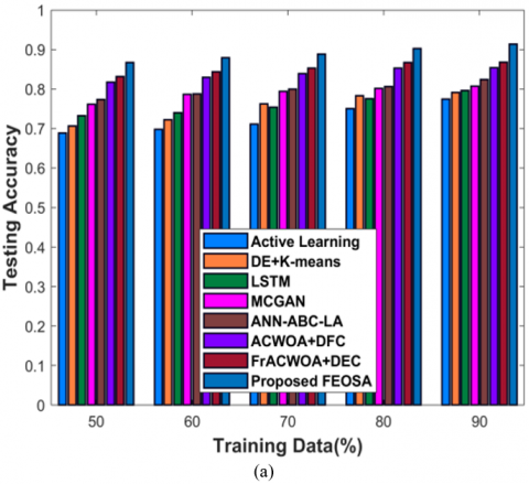
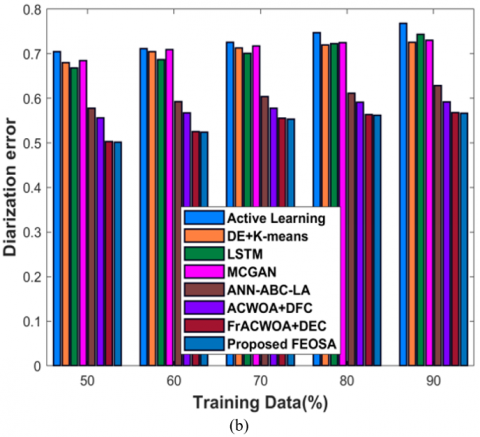
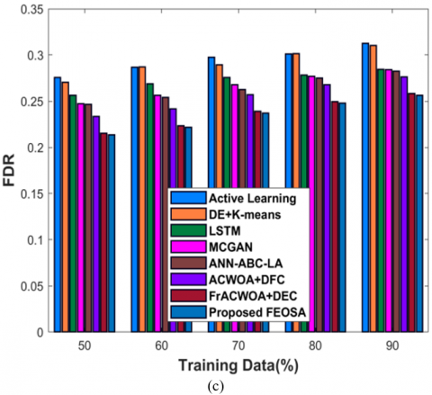
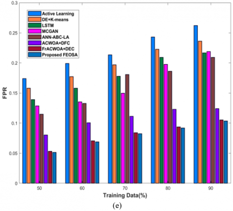
In Figure 4 a), evaluation of proposed FEOSA with respect to testing accuracy is displayed. If training data=90%, accuracy gained by designed scheme is 0.913 that delivers performance enhancement of devised approach to that of existing models, is 15.218%, 13.395%, 12.817%, 11.640%, 9.801%, 6.511%, and 4.987%. Figure 4 b) represents the analysis of diarization error. The FEOSA achieved diarization error as 0.566, whereas the classical schemes delivered the diarization error as 0.768for active learning, 0.725 for DE + K-means, 0.743 for LSTM, 0.730 for MCGAN, 0.629 for ANN-ABC-LA, 0.592 for ACWOA+DFC, and 0.568 for FrACWOA+DEC for data=90%. Figure 4 c) reveals the assessment of modeled approach in respect to FDR. For training percentage=90%, FDR attained by proposed FEOSA is 0.257 and the FNR obtained by FEOSA is 0.128 as shown in Figure 4 d). Figure 4 e) displays the evaluation of FPR. While increasing 90%, FPR attained by developed approach is 0.104, while conventional schemes obtained the FPR of 0.262, 0.236, 0.217, 0.219, 0.209, 0.124, and 0.105, respectively C.
4.6.2 Assessment based on test case-1 by varying K-fold
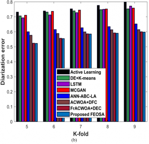
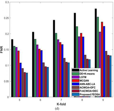
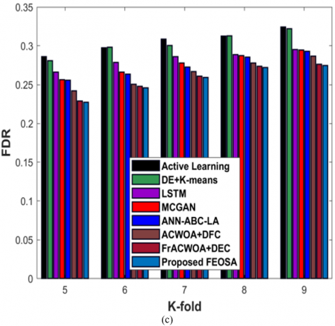
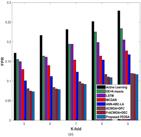
Figure 5 a) implies the estimation of designed FEOSA in respect to testing accuracy by changing K-fold value. If K-fold is 9, accuracy yielded by devised approach is 0.924. The existing techniques gained K-fold value as 0.804 for active learning, 0.822 for DE + K-means, 0.827 for LSTM, 0.838 for MCGAN, 0.856 for ANN-ABC-LA, 0.887 for ACWOA+DFC, and 0.902 for FrACWOA+DEC. If the K-fold measure is 9, diarization error attained by FEOSA is 0.598 depicted in Figure 5 b). Figure 5 c) implies the estimation of developed FEOSA in regard to FDR. If K-fold value as 9, FDR revealed by modeled strategy is 0.265. Figure 5 d) and 5 e) signifies the estimation of designed scheme in accordance with FNR and FPR. ForK-fold value=9, FNR gained by proposed approach is 0.131, while the proposed FEOSA delivered FPR as 0.106.
4.6.3 Assessment based on testcase-2 by varying training data
Figure 6 a) reveals estimation of proposed FEOSA in accordance to testing accuracy. For training data=90%, accuracy gained by developed model is 0.880 that outcomes the evolvement of proposed approach to that of existing models is 19.719%, 16.741%, 13.492%, 10.304%, s 9.220%, 3.778%, and 1.426%. Figure 6 b) depicts the evaluation of diarization error. The FEOSA achieved diarization error as 0.628, whereas the classical techniques provided the diarization error as 0.801 for active learning, 0.757 for DE + K-means, 0.776 for LSTM, 0.762 for MCGAN, 0.656 for ANN-ABC-LA, 0.618 for ACWOA+DFC, and 0.630 for FrACWOA+DEC for data=90%. Figure 6 c) reveals the estimation of modeled scheme in relation to FDR. For training data=90%, FDR attained by proposed FEOSA is 0.266 and the FNR obtained by proposed model is 0.114 as displayed in Figure 6 d). Figure 6 e) portrays the assessment of FPR. While taking the data as 90%, FPR attained by modeled approach is 0.114, while conventional schemes showed the FPR of 0.270, 0.226, 0.199, 0.172, 0.163, 0.117, and 0.115.
4.6.4 Estimation based on test case-2 by varying K-fold value
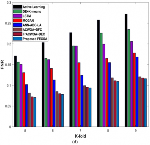
Figure 7 a) specifies the estimation of FEOSA with respect to testing accuracy by changing K-fold value. If K-fold measure is 9, accuracy yielded by developed work is 0.922. However, existing techniques gained the K-fold value as 0.785 for active learning, 0.809 for DE + K-means, 0.815 for LSTM, 0.835 for MCGAN, 0.863 for ANN-ABC-LA, 0.884 for ACWOA+DFC, and 0.903 for FrACWOA+DEC. For K-fold value is 9, diarization error attained by FEOSA is 0.626 illustrated in Figure 7 b). Figure 7 c) implies the estimation of developed FEOSA in terms of FDR. While considering the K-fold value as 9, FDR gained by designed strategy is 0.275, while the classical models attained the FDR value as 0.324 for active learning, 0.322 for DE + K-means, 0.295 for LSTM, 0.295 for MCGAN, 0.293 for ANN-ABC-LA, 0.287 for ACWOA+DFC, and 0.276 for FrACWOA+DEC. Figures 7 d) and 7 e) signifies the estimation of FEOSA model in terms of FNR and FPR. ForK-fold value=9, FNR gained by proposed approach is 0.116. On the other hand, FEOSA gained FPR as 0.116.
Figure 4. Estimation based on testcase-1 with training data, a) Testing accuracy, b) Diarization error, c) FDR, d) FNR, e) FPR
Figure 5. Evaluation based on testcase-1 with K-fold value, a) Testing accuracy, b) Diarization error, c) FDR, d) FNR, e) FPR
Figure 6. Estimation based on testcase-2 with training data, a) Testing accuracy, b) Diarization error, c) FDR, d) FNR, e) FPR
Figure 7. Evaluation based on testcase-1 with K-fold value, a) Testing accuracy, b) Diarization error, c) FDR, d) FNR, e) FPR
Table 1. Comparative discussion
|
Test Cases |
Metrics/Methods |
Active Learning |
DE+K-Means |
LSTM |
MCGAN |
ANN-ABC-LA |
ACWOA+DFC |
FrACWOA+DEC |
Proposed FEOSA |
|
Test case-1 Training data=90% |
Testing accuracy |
0.774 |
0.791 |
0.796 |
0.807 |
0.824 |
0.854 |
0.868 |
0.913 |
|
Diarization error |
0.768 |
0.725 |
0.743 |
0.730 |
0.629 |
0.592 |
0.568 |
0.566 |
|
|
FDR |
0.312 |
0.310 |
0.285 |
0.284 |
0.282 |
0.276 |
0.258 |
0.257 |
|
|
FNR |
0.270 |
0.245 |
0.200 |
0.230 |
0.217 |
0.141 |
0.129 |
0.128 |
|
|
FPR |
0.262 |
0.236 |
0.217 |
0.219 |
0.209 |
0.124 |
0.105 |
0.104 |
|
|
Test case-1 K-fold value=9 |
Testing accuracy |
0.804 |
0.822 |
0.827 |
0.838 |
0.856 |
0.887 |
0.902 |
0.924 |
|
Diarization error |
0.798 |
0.753 |
0.772 |
0.758 |
0.653 |
0.615 |
0.600 |
0.598 |
|
|
FDR |
0.323 |
0.321 |
0.294 |
0.294 |
0.292 |
0.286 |
0.267 |
0.265 |
|
|
FNR |
0.279 |
0.253 |
0.206 |
0.237 |
0.224 |
0.145 |
0.132 |
0.131 |
|
|
FPR |
0.271 |
0.244 |
0.224 |
0.226 |
0.216 |
0.127 |
0.107 |
0.106 |
|
|
Test case-2 Training data=90% |
Testing accuracy |
0.788 |
0.811 |
0.817 |
0.837 |
0.866 |
0.886 |
0.905 |
0.922 |
|
Diarization error |
0.801 |
0.757 |
0.776 |
0.762 |
0.656 |
0.618 |
0.630 |
0.628 |
|
|
FDR |
0.314 |
0.311 |
0.286 |
0.285 |
0.284 |
0.278 |
0.267 |
0.266 |
|
|
FNR |
0.263 |
0.227 |
0.200 |
0.173 |
0.164 |
0.118 |
0.115 |
0.114 |
|
|
FPR |
0.270 |
0.226 |
0.199 |
0.172 |
0.163 |
0.117 |
0.115 |
0.114 |
|
|
Test case-2 K-fold value=9 |
Testing accuracy |
0.785 |
0.809 |
0.815 |
0.835 |
0.863 |
0.884 |
0.903 |
0.922 |
|
Diarization error |
0.799 |
0.755 |
0.773 |
0.759 |
0.654 |
0.616 |
0.628 |
0.626 |
|
|
FDR |
0.324 |
0.322 |
0.295 |
0.295 |
0.293 |
0.287 |
0.276 |
0.275 |
|
|
FNR |
0.272 |
0.235 |
0.206 |
0.178 |
0.168 |
0.121 |
0.118 |
0.116 |
|
|
FPR |
0.279 |
0.233 |
0.205 |
0.177 |
0.167 |
0.119 |
0.118 |
0.116 |
4.7 Comparative discussion
Table 1 shows the discussion of FEOSA. Accordig to the discussion conducted, it is comprehensible that FEOSA has resulted superior performance with excellent results in term sof accuracy while segmenting the speech and performing the speech diarization task. It is declared that FEOSA has provided high testing accuracy of 0.913, minimum diarization error of 0.566, FDR of 0.257, FNR of 0.128, and FPR of 0.104 for test case-1 while considering training data as 90%.
Most of the speaker diarization investigation has concentrated on unsupervised cases, where no manual supervision is existing. Nevertheless, the huge challenge exists on minimizing the manual supervision to improve the system performance.
This research provides a solution to speaker segmentation and diarization using proposed FEOSA, which is a combination of FC and EOSA. The gist of this article is to model an effective pipeline for speaker segmentation and diarization using designed FEOSA. Here, the features like MFCC, LPCC, LSF, spectral roll off, logarithmic band power, spectral skewness, zero-crossing rate, FFT, spectral centroid and power spectral density are refined by taking the audio signal as an input.
The, speech activity identification is done to extract the speech signal from non-speech signals, such as noises, background music and so on. The next step is the speaker segmentation phase, which is accomplished based on speaker change identification and constant thresholds are computed based on proposed FEOSA.
At last, speaker diarization is conducted using entropy weighted power k-means and the weights are upgraded utilizing FEOSA. The proposed FEOSA has attained maximum testing accuracy of 0.913, minimum diarization error of 0.566, FDR of 0.257, FNR of 0.128, and FPR of 0.104 for test case-1 while considering the training data as 90%. Despite the growth in high-quality speaker diarization algorithms, there are still many issues that should be rectified immediately, such as overlapping speech or speakers voice modulations and this topic would be regarded as a potential future investigation area.
[1] Sun, H., Ma, B., Khine, S.Z.K., Li, H. (2010). Speaker diarization system for RT07 and RT09 meeting room audio. In IEEE International Conference on Acoustics, Speech and Signal Processing,Dallas, TX, USA, pp. 4982-4985. https://doi.org/10.1109/ICASSP.2010.5495077
[2] Meignier, S., Moraru, D., Fredouille, C., Bonastre, J.F., Besacier, L. (2006). Step-by-step and integrated approaches in broadcast news speaker diarization. Computer Speech & Language, 20(2-3): 303-330. https://doi.org/10.1016/j.csl.2005.08.002
[3] VijayKumar, K., Rao, R.R. (2023). Optimized speaker change detection approach for speaker segmentation towards speaker diarization based on deep learning. Data & Knowledge Engineering, 144: 102121. https://doi.org/10.1016/j.datak.2022.102121
[4] Ramaiah, V.S., Rao, R.R. (2018). Speaker diarization system using HXLPS and deep neural network. Alexandria Engineering Journal, 57(1): 255-266. https://doi.org/10.1016/j.aej.2016.12.009
[5] Xu, Y., McLoughlin, I., Song, Y., Wu, K. (2016). Improved i-vector representation for speaker diarization. Circuits, Systems, and Signal Processing, 35(9): 3393-3404. https://doi.org/10.1007/s00034-015-0206-2
[6] Ahmad, R., Zubair, S., Alquhayz, H., Ditta, A. (2019). Multimodal speaker diarization using a pre-trained audio-visual synchronization model. Sensors, 19(23): 5163. https://doi.org/10.3390/s19235163
[7] Tranter, S.E., Reynolds, D.A. (2006). An overview of automatic speaker diarization systems. IEEE Transactions on Audio, Speech, and Language Processing, 14(5): 1557-1565. https://doi.org/10.1109/TASL.2006.878256
[8] Ahmad, R., Zubair, S., Alquhayz, H. (2020). Speech enhancement for multimodal speaker diarization system. IEEE Access, 8: 126671-126680. https://doi.org/10.1109/ACCESS.2020.3007312
[9] Moattar, M.H., Homayounpour, M.M. (2012). A review on speaker diarization systems and approaches. Speech Communication, 54(10): 1065-1103. https://doi.org/10.1016/j.specom.2012.05.002
[10] Karim, D., Salah, H., Adnen, C. (2019). Hybridization DE with K-means for speaker clustering in speaker diarization of broadcasts news. International Journal of Speech Technology, 22(4): 893-909. https://doi.org/10.1007/s10772-019-09633-6
[11] Rokach, L., Maimon, O. (2005). Clustering methods. In Data Mining and Knowledge Discovery Handbook, Boston, MA, pp. 321-352. https://doi.org/10.1007/0-387-25465-X_15
[12] Wang, J., Xiao, X., Wu, J., Ramamurthy, R., Rudzicz, F., Brudno, M. (2020). Speaker diarization with session-level speaker embedding refinement using graph neural networks. In ICASSP IEEE International Conference on Acoustics, Speech and Signal Processing (ICASSP), Barcelona, Spain, pp. 7109-7113. https://doi.org/10.1109/ICASSP40776.2020.9054176
[13] Snyder, D., Garcia-Romero, D., Sell, G., Povey, D., Khudanpur, S. (2018). X-vectors: Robust DNN embeddings for speaker recognition. In IEEE International Conference on Acoustics, Speech And Signal Processing (ICASSP), Calgary, AB, Canada, pp. 5329-5333. https://doi.org/10.1109/ICASSP.2018.8461375
[14] Sainath, T., Weiss, R.J., Wilson, K., Senior, A.W., Vinyals, O. (2015). Learning the speech front-end with raw waveform CLDNNs. Google, Inc. New York, NY, USA.
[15] Vasamsetti, S., Santhirani, C. (2020). Hybrid particle swarm optimization-deep neural network model for speaker recognition. Multimedia Research, 3(1): 1-10
[16] Ravanelli, M., Bengio, Y. (2018). Speaker recognition from raw waveform with sincnet. In IEEE Spoken Language Technology Workshop (SLT), Athens, Greece, pp. 1021-1028. https://doi.org/10.1109/SLT.2018.8639585
[17] Dubey, H., Sangwan, A., Hansen, J.H. (2019). Transfer learning using raw waveform sincnet for robust speaker diarization. In ICASSP 2019-2019 IEEE International Conference on Acoustics, Speech and Signal Processing (ICASSP), Brighton, UK, pp. 6296-6300. https://doi.org/10.1109/ICASSP.2019.8683023
[18] Anita, J.S., Abinaya, J.S. (2019). Impact of supervised classifier on speech emotion recognition. Multimedia Research, 2(1): 9-16.
[19] Pal, M., Kumar, M., Peri, R., Park, T.J., Kim, S.H., Lord, C., Bishop, S., Narayanan, S. (2021). Meta-learning with latent space clustering in generative adversarial network for speaker diarization. IEEE/ACM Transactions on Audio, Speech, and Language Processing, 29: 1204-1219. https://doi.org/10.1109/TASLP.2021.3061885
[20] Pal, M., Kumar, M., Peri, R., Park, T.J., Kim, S.H., Lord, C., Bishop, S., Narayanan, S. (2020). Speaker diarization using latent space clustering in generative adversarial network. In ICASSP 2020-2020 IEEE International Conference on Acoustics, Speech and Signal Processing (ICASSP), Barcelona, Spain, pp. 6504-6508. https://doi.org/10.1109/ICASSP40776.2020.9053952
[21] Dasari, K.B., Devarakonda, N. (2021). Detection of different DDoS attacks using machine learning classification algorithms. Ingénierie des Systèmes d’Information, 26(5): 461-468. https://https://doi.org/10.18280/isi.260505
[22] Oyelade, O.N., Ezugwu, A.E. (2021). Ebola Optimization Search Algorithm (EOSA): A new metaheuristic algorithm based on the propagation model of Ebola virus disease. arXiv preprint arXiv:2106.01416. https://doi.org/10.48550/arXiv.2106.01416.
[23] EenaduPrathidwani dataset taken from: https://www.etv.co.in/showsentitys.
[24] Jin, Q., Schultz, T. (2004). Speaker segmentation and clustering in meetings. Interspeech, 4: 597-600
[25] Chakraborty, S., Paul, D., Das, S., Xu, J. (2020). Entropy-weighted power k-means clustering. In International Conference on Artificial Intelligence and Statistics, pp. 691-701
[26] Sharma, G., Umapathy, K., Krishnan, S. (2020). Trends in audio signal feature extraction methods. Applied Acoustics, 158: 107020. https://doi.org/10.1016/j.apacoust.2019.107020
[27] Dasari, K.B., Devarakonda, N. (2022). Detection of TCP-based DDoS attacks with SVM classification with different kernel functions using common uncorrelated feature subsets. International Journal of Safety and Security Engineering, 12(2): 239-249. https://doi.org/10.18280/ijsse.120213
[28] Itoh, T., Yamauchi, N. (2007). Surface morphology characterization of pentacene thin film and its substrate with under-layers by power spectral density using fast Fourier transform algorithms. Applied Surface Science, 253(14): 6196-6202. https://doi.org/10.1016/j.apsusc.2007.01.056