Roohi Sille* | Tanupriya Choudhury | Piyush Chauhan | Durgansh Sharma
© 2021 IIETA. This article is published by IIETA and is licensed under the CC BY 4.0 license (http://creativecommons.org/licenses/by/4.0/).
OPEN ACCESS
Magnetic resonance Imaging (MRI) is one of the most utilized medical imaging techniques for detecting and diagnosing the different abnormalities such as tumors, lesions within various internal organs of human body. Manual segmentation from these images is time-consuming and complex. Due to this, automatic segmentation techniques such as convolutional neural network (CNN), deep neural networks are used. An accurate, efficient and advanced computational segmentation method is extremely required for fatal diseases like brain tumor from brain MRI images. In this research work, deep learning model comprising of three channels such as patch extraction, 6 layered transfer-learning capsule and 5 layered segmentations capsule This proposed work addresses deep learning coupled with small kernels and handles the obstacles in brain tumor segmentation techniques. The proposed model is a 11-layered deep capsule network consisting of transfer learning along with two dropout layer at the input and 5 layers of segmentation channel along with dropout layers. The work presented in this paper focusses in attaining a high dice score coefficient and accuracy in brain tumor segmentation from MRI images. The model presented in this paper is effectively trained over 150 images in the dataset. The proposed work has attained comparative better results with respect to the dice score coefficient such as (0.80, 0.76, 0.76) for whole tumor [WT], active tumor [AT] and core tumor [CT] respectively.
deep neural networks, segmentation algorithm, transfer learning algorithm, brain tumor, deep capsule network
Brain Tumor or Intracranial neoplasm arises due to anomalous cells that emerge within the brain. Due to the complex and time-consuming nature of manual segmentation of brain tumors from MRI images, automatic segmentation is preferred. Immense research is going on in the field of automatic segmentation of brain tumors. Brain tumors prove to be fatal for human health and leads to death of the person. To decrement the death rate, early diagnosis of brain tumors is much required. Automatic segmentation leads to early diagnosis of tumors in MRI images due to the smaller amount of diagnostic time. Recent research focusses on designing efficient and accurate automated segmentation techniques, amongst which deep learning techniques plays a vital role in efficient brain tumor segmentation. There are various deep learning techniques such as deep belief networks (DBN), stacked autoencoders (SAE) and convolutional Neural Network (CNN) utilized for brain tumor segmentation. Convolutional Neural Networks have attained the most accurate results and hence are effectively used for segmentation of brain tumors from MRI images [1]. It is a feed-forward neural network consisting of multiple layers such pooling, convolutional and fully convolutional layer. To attain higher dice score coefficient in segmentation algorithm, parameters of these layers along with different weights and bias are modified.
Gliomas are most communal and destructive types of tumors in brain. These tumors lead to high mortality and morbidity. It is divided into high-grade gliomas (HGG) and low-grade gliomas (LGG) [2]. The sub-regions of a brain tumor are necrosis and edema, necrosis is the dead part and edema is the swelling caused by tumor which is subdivided into enhancing and non-enhancing tumors [3, 4]. All these sub-regions combined together represents whole tumor (WT) whereas the non-enhancing and enhancing concludes in core tumor (CT) and enhancing region describes the active tumor (AT) [5, 6]. Active tumor is a subset of core tumor and core tumor is a subset of whole tumor.
These tumors are detected by different imaging modalities such as magnetic resonance imaging (MRI), positron electron tomography (PET), computed tomography scan (CT scan), etc. Amongst these, Magnetic resonance imaging (MRI) has attained good results in detection and diagnosis if patient’s health condition due to its capability of providing a good contrast for soft tissues as compared to other imaging modalities. In addition, there are no known health hazards from temporary exposure to MR environment. Therefore, MRI is a good technique for accessing brain tumor in human beings. Manual anomaly detection from magnetic resonance imaging (MRI images) is complex and time-consuming process. Anomalies such as tumors require early detection and immediate medical care, which is tough in case of manual segmentation. Due to these reasons, automatic segmentation algorithms with higher dice score coefficient have proven to be the best diagnosis for brain tumor segmentation. Magnetic resonance imaging helps in locating multiple modalities of tumor tissues and tumor effect in different tissues including T1 weighted, T1c weighted, T2 and Fluid Attenuated Recovery inversion (FLAIR). These multiple modalities are differentiated amongst contrast and brightness of Magnetic resonance images [7, 8]. These modalities are very sensitive due to the tissues affected by inflammation and are associated directly to pathology [9]. Amongst these modalities, T1 weighted is the most common modality mainly used for structural analysis and differentiating healthy and unhealthy tissues. Due to the prominent nature of gliomas, highest morbidity rate is possessed [10]. T1 weighted presents an enhanced brain tumor segmentation technique based on the gradient and the context-sensitive attributes [2] to detect diverse tumor cells for high grade gliomas and low grade. In T1c modality, glioblastoma is enriched from the borders. For segregating active tumors (AT) from necrotic region, T1c weighted modality is effective used. The edema portion or the core tumor (CT) in the T2 appears much brighter [11]. For identification of whole tumor, fluid attenuation inversion recovery (FLAIR) is utilized. In the dataset, for each patient, images from different sequences namely: T1, T2-contrasted and FLAIR (Fluid Attenuated Inversion Recovery) acquired. Each of these sequences exploits the distinct characteristics of the tissues as explained above which results in contrast among the images. For better segmentation results, the contrast values of all the image modalities are extracted that exploit distinct characteristics of the tissues. As shown in the figure below, the WT (whole tumor) is perceptible clearly in the sequence Flair Figure 1. The CT (core tumor) is visible in the sequence T2 and the ET (enhancing tumor) structure is visible in the Figure 1. Due to this, we need MR images from different sequences so that we can identify/classify the intra-tumor structure precisely [12, 13].
Figure 1. Different MRI sequences
In earlier segmentation algorithms, handcrafted features were extracted manually hence increased level of complexity. Deep learning ha seduced the complexity of extracting features manually as in deep learning segmentation algorithms features are extracted directly from the data with increasing hierarchy. Therefore, instead of going in regular way that is manual feature extraction, our objective should be in developing more effective deep architectures that learn the features within itself. This is one of the major reasons of using deep learning for solving problems such as extraction features of tumor from brain images.
Detection of tumor is a very challenging and intuitive task due to the variation of tumor’s features such as location, shape an structure from patient to patient. This leads to a very challenging task of segmenting tumors among various Magnetic resonance images (MRI) [14]. In the Figure 2, some images of the same brain slice from different patients are shown, that reflects the tumor variation. We can clearly see that the location of tumor is different in all the eight images or patients shown below. To make it worse, the shape and the intra-tumor structure is also different from all the eight images (Figure 2). In fact, there can be more than one region of tumor as seen from the images below [15, 16]. This indeed reflects the complexity of automatic segmentation.
Figure 2. Tumor in different patients for the same brain slice
Dice score is the evaluator for the performance attained by segmentation techniques or algorithm. It is estimated by Dice Similarity Coefficient (DSC) [2], which compute the imbricate between the automatic and the manual segmentation.
$D S C=\frac{2 T P 1}{(F P 1+2 T P 1+F N 1)}$ (1)
Here, FP1 represents False Positive, TP1 represents True Positive, and FN1 represents False Negative [2, 17].
This paper discusses some of the essential concepts of multilayer perception in convolutional neural network (CNN) and deep convolutional neural networks particularly utilized for brain tumor segmentation [18, 19]. The major challenge with assessment of these segmentation algorithms is evaluating the Dice Score [20-22].
In summary, this paper has the following contributions: i) A deep capsule convolutional neural network (CNN) to fully extract high level features from brain magnetic resonance images is proposed. ii) Two capsules: transfer learning algorithm and segmentation algorithm along with different dropout layers have been proposed. iii) The performance of deep capsule network is investigated on brain tumor segmentation dataset. The results show that deep capsule network significantly outperform deep CNN.
Recent research has focused on the deep learning methods implemented for segmenting brain tumor from magnetic resonance images. In this section, a formal summary and brief description of deep learning models such as Stacked auto encoders, restricted botlzman’s machine, deep belief networks and convolutional neural networks, is discussed. This literature survey enhances the future trends for brain tumor segmentation based on the past trends.
Auto encoder’s and stacked auto-encoders (deep AEs or SAE): In these networks, the auto encoder layers are stacked together and trained independently for fine-tuned prediction using supervised learning [23]. These simple networks are assisted by a weight matrix w and bias b gathered from input along with parallel bias from hidden layer refined to hidden state for the remodeling. Hidden activation $h_{l}$ is calculated by a nonlinear activation function $\sigma$:
$h_{l}=\sigma\left(w_{i, h} i+b_{i, h}\right)$ (2)
A method was proposed for generating a noise free input to avoid the model from adapting an insignificant solution [24].
In Deep Belief Networks (DBN), densely connected neurons lead to rapid and accurate learning of relevant features. Due to the difficulty in learning with these nets with multiple hidden layers, a fast and greedy algorithm is proposed for DBN (deep belief nets) [25, 26].
The Restricted Boltzmann’s Machine (RBM) resemble to Markov random fields consisting of input layer, hidden layer that outputs hidden feature representation. Due to the bidirectional nature of nodes, latent feature representation is extracted from an input vector and vice versa. An energy function, e is defined for a precise state of IU (input units) and HU (hidden units).
$e(i, h)=h^{T} w i-c^{T} i+b^{T} i$ (3)
where, B and c are bias terms. The probability P(i,h) of the state of the system is calculated as follows:
$P(i, h)=\frac{1}{p} \exp \{-e(i, h)\}$ (4)
The partition function p is evaluated inflexibly. However, restricted inference of calculating trained on or vice versa is flexible and results as follows:
$p\left(h_{j} \mid i\right)=\frac{1}{1+\exp \left\{-b_{j}-w_{j} i\right\}}$ (5)
Deep Belief networks and stacked auto-encoders are differentiated based on the layers that is auto encoder layers of stacked auto-encoders are substituted by restricted boltzman’s machine.
Convolutional Neural Networks: The convolution operation is performed with a set of n kernels with weights w and added biases b individually creating a new feature map on the input image at each layer. These features forced to an element-by-element nonlinear transform for every convolutional layer L:
$\mathrm{f}_{\mathrm{n}}^{\mathrm{L}}=\sigma\left(\mathrm{w}_{\mathrm{n}}^{\mathrm{L}-1} * \mathrm{f}^{\mathrm{L}-1}+\mathrm{b}_{n}^{\mathrm{L}-1}\right)$ (6)
A 6- layered 3D CNN comprising of global CNN and local CNN proposed to perform striatum segmentation. This model incorporates a dropout layer for reducing overfitting and learning more robust features. The T1 modality of magnetic resonance imaging are input to global CNN for determining the approximate location of stratum and this output is shared as input to local CNN where the volume of stratum is extracted. This model obtained higher dice similarity coefficient and precision score [27, 28].
A multi modal 2D CNN’s and multi scale late fusion CNN was proposed for magnetic resonance image segmentation for feature extraction and generating feature maps. These methods led to better and efficient segmentation quality [29, 30].
A multi scale, CNN was proposed for lesion segmentation on non-uniform area to incorporate anatomical location information into the network. This method was used for segmentation of white matter intensities [31]. Fully convolutional network with 3D CNN reduced false positives and 3worked for brain extraction from multimodal input. These methods attained average dice score, high specificity and average sensitivity [32, 33].
Hough-voting CNN’s was proposed for full patch segmentations which attained robust, flexible and efficient results for multi-modal segmentation [34-38].
A 3D FCN trailed with 3D CNN is proposed for candidate segmentation for reduction in false positives. It also utilizes spatial information for extraction of high-level features hence achieve much better detection accuracy [39-42].
A Segnet named deep neural network introduced for automatic segmentation of Brain MRI. Segnet allocates each voxel to its equivalent anatomical region in an MR image of the brain. Non-linear registration of MRI is not required in this network [43].
A DCENN (deep convolutional encoder neural network) segments brain lesions from magnetic resonance images of brain [44]. This model boosts the training by gathering features from entire images, which abolishes patch selection and iterating computations at the intersection of neighboring patches.
A 11-layered deep, double-pathway, 3D CNN, developed for the separation of brain lesions [45]. When multi modal 3D patch processes at multiple scales within the developed system, it fragments voxel-wise pathology. This network processes a 3D brain volume in 3 minutes. Conditional random fields were later added to the network for enhancing the results.
A multi-cascaded architecture along with conditional random fields (CRF’s) was developed for coarse to fine segmentation by adopting multiscale features [46, 47].
A nnUnet was modified with post processing algorithm to attain a higher dice score coefficient values f 88.95, 85.06 and 82.03 for whole tumor, tumor core and enhancing tumor, respectively [48].
A Dilated Dense Attention Unet (DDAUnet) proposed for computed tomography scans that benefits in spatial and channel attention gates in several dense block to collectively examine on fixed feature maps and regions. Dilated convolutional layers are used to supervise GPU memory and enhance the network receptive field The proposed network attained a DSC value of 0.79 ± 0.20 [49].
Below Table 1 summarizes the literature review on brain tumor segmentation algorithms.
Based on the related works, deep convolutional neural networks have proven to attain a state of art in brain tumor segmentation task. Dual pathway Convolutional neural networks have given high specificity, sensitivity and dice score coefficient, hence resulting in excellent segmentation. Due to the high memory consumption by medical images, the models are designed by extracting patches (pixel patch for two-dimensional images and voxel patch for three dimensional images) initially and hence extracting accurate feature maps. Accurate feature mapping leads towards better accuracy than directly feeding complete image within the convolutional neural network. Some of the work has also been done on voxel wise convolutional neural network (CNN) that attained similar results as patch based extraction. These deep learning algorithms can be evaluated based on following performance parameters such as dice similarity coefficient, sensitivity, similarity index and accuracy, precision [50]. The proposed model has included both dual convolutional neural network model and patch extraction to enhance the dice score coefficient.
Table 1. Deep learning algorithms with its advantages
|
Algorithms |
Advantages |
|
6 layered 3DCNN [29] |
Reduced overfitting Learn more robust features |
|
Multimodal 2d CNN [30] |
Better for infant brain segmentation |
|
multi scale late fusion CNN [31] |
Better and efficient segmentation quality |
|
Deep voxelwise residual network VoxResNet [3] |
refining the volumetric segmentation performance |
|
Multi scale, CNN [32, 33] |
reduced false positives |
|
3D fully CNN [34] |
average dice score, high specificity and average sensitivity |
|
Hough-voting CNN [35, 36] |
attained robust, flexible and efficient results |
|
Segnet [44] |
Non-linear registration of MRI is not required |
|
DCENN [45] |
speeds up the training |
|
Double-pathway, 3D CNN [46] |
processes a 3D brain volume in 3 minutes |
|
3 CNN architectures
|
The first two architectures performed well with a dice score of 0.84 and 0.86 respectively as compared to the third architecture. |
|
3D FCN trailed with 3D CNN |
achieve much better detection accuracy |
|
Multi-cascade CNN with CRF’s [48] |
Attained quantitative and qualitative segmentation results |
|
nnUnet [49] |
Attained quantitative and qualitative results along with post processing method |
|
Dilated Dense Attention Unet (DDAUnet) [50] |
Improve extracted features and hence enhanced the segmentation results. |
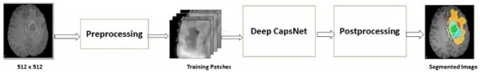
According to the literature survey, deep CNN has proven to be the state of art for brain tumor segmentation. The proposed work focusses on attaining good segmentation results by achieving good dice score coefficient. Based on the related literature, proposed work has included patch based segmentation along with transfer learning based on convolutional neural networks. The proposed model is a 11-layered capsulated convolutional neural network architecture [51]. The first capsule incorporates transfer learning layer three convolutional layers with two dropout layer, one max-pooling layer followed by two convolutional layers. The second capsule incorporates segmentation layers comprising one convolutional layer, one max-pooling layer and three fully convolutional layers with two dropout layers. The patch extraction helps in extracting high level features and transfer learning approach has improved the performance of the proposed model. Figure 3 shows the overview of the proposed model. In the proposed model, we have implemented different patch extraction methods, the output of which is fed to the CNN and processed with the help of transfer learning algorithm.
a.) Pre-processing is one the challenging task in dealing with the MRI data, due to the inhomogeneity within tumor scans caused by various movements of the magnetic fields [52]. The presence of bias across the patients MRI scans causes difficulty in fetching accurate segmentation results. Same tissues vary a lot in intensity values from time to time because of the bias field distortion. This error of bias field distortion can be removed by N4TK algorithm in bias field correction [53, 54].
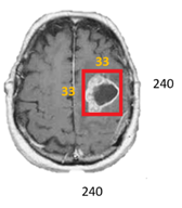
b.) For intensity normalization of the images across the multiple patients, a two-step method has been implemented [2, 19] that is the training step and the transformation step. The training step is executed only once for a given dataset and the lateral is executed for each image in the dataset. To fetch the intensity values corresponding to each landmark location including mapping of these locations is done by this training and transformation stage [55]. As shown in the Figure 4, 33 x 33 patch is extracted from 240x240 image .in the transformation phase. These are matched to several linear mappings from one point to another.
Patch extraction helps in reduction in number of parameters so that the complexity of convolutional neural network is reduced. In this proposed work, patch of size 33×33 is selected from an image of size 240×240. This leads to a selected number of high level parameters required by the model for segmenting tumors. The given voxel category is directly proportional with the neighbour voxels category. In the proposed model, patches are used for training purpose. At the testing stage, the patch size of 33×33 works fine with the dataset obtained.
c.) Due to the patch extraction method, dataset has been reduced. For enlarging the training dataset by 10 fold, data augmentation has been applied in the model. This technique is not effective for a larger dataset. In this work, rotation and flipping are performed randomly at runtime in the training dataset to generate new dataset. Some samples (t) are randomly selected from the batch size of 128 and one of the three operations like rotation, horizontal and vertical flip is randomly applied. Some modified samples are also collected by randomly combining two operations out of three. These modified samples are merged with ‘t’ to form the training set.
Figure 3. Proposed model (Deep capsule network)
Figure 4. Patch extraction
Figure 5. Convolution of image
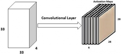
In the proposed model, a 5×5 ×3 filter is slid over an image, and the dot product is calculated in the convolutional layer. This results in the generation of a new image. This output image is known as an activation map as shown in Figure 5. In the proposed model, the achieved activation map was of size 28×28×1 as shown in Figure 6. These filters are assigned either randomly or based on the parameters.
Figure 6. Convolution with multiple filters
Pooling layer helps to reduce the spatial size by reducing the number of parameters. In proposed model, max-pooling is used. It is important to use max-pooling layer in between convolutional layers as it helps in reduction of unwanted parameters.
|
Deep Capsule Network |
|
Input: Image X: 512 x 512 Output: Segmented Image, Xs -> 240 x 240 Method: Start
End X=input image, Xs ->segmented image, Xp->extracted patch, Xn-> generated new image, Xa->activation map, Xr->convolved output, Xrp->Max-pooling output |
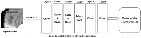
d.) Transfer learning algorithm helps in improving the learning curve by transferring the knowledge from a trained convolutional neural network model to a test model [56]. Its same as transferring knowledge from humans to the machine so that machines work take decisions, search patterns etc. exactly like humans. This knowledge helps in analysing different humans at different age levels [57]. In proposed work, transfer learning model comprises initially of three convolutional layers then max-pooling layer followed by one more convolutional layer. The output of transfer learning algorithm in the form of vector of size 128×16×16 is transferred to segmentation algorithm. The proposed model for brain tumor segmentation is 11- layered architecture consisting of transfer learning layer and segmentation layer encapsulated together. The transfer learning CNN model is shown in Figure 7 and detailed configuration is mentioned in Table 2.
Figure 7. Transfer learning CNN model
Table 2. Transfer learning CNN model chart
|
Layers |
Input |
Filter size |
Stride |
Filters |
Dropout Rate |
|
Convolutional |
4×33×33 |
3×3 |
1×1 |
128 |
NR* |
|
Convolutional + dropout |
NR* |
3×3 |
2×2 |
NR* |
0.8 |
|
Convolutional + dropout |
NR* |
3×3 |
2×2 |
NR* |
0.8 |
|
Max-pooling |
NR* |
3×3 |
2×2 |
NR* |
NR* |
|
Convolutional |
128×16×16 |
NR* |
NR* |
NR* |
NR* |
|
Convolutional |
128×16×16 |
3×3 |
2×2 |
NR* |
NR* |
*NR-Not Reported
e.) Segmentation algorithm comprises of one convolution layer, one max-pooling layer and three fully convolutional layer. Below is the CNN model comprising of the five layers such as convolutional layer, max-pooling layer and the three fully convolutional layer. A small kernel of 3×3 is used as a filter in convolutional and max-pooling layer and dropout of rate 0.5 is used in two fully convolutional layers. The segmentation layer CNN model is shown in Figure 8 and detailed configuration of model is shown in Table 3.
Figure 8. Segmentation layer
In medical image segmentation using a convolutional neural network, overfitting is the major obstacle towards excellent results [58]. While training the network, the error values are stored and mapped with the new data obtained for comparison. The compared result might vary or can be large as well is termed as overfitting. In the proposed model, a dropout layer is used to reduce this overfitting issue. The dropout layer having dropout rate of 0.8 is used in transfer learning layer. Another dropout layer having dropout rate of 0.5 in segmentation layer. The dropout rate has a significant result on layers of retrained convolutional neural network (CNN) based on transfer learning and complexity of segmentation layers [59].
Table 3. Segmentation layer CNN model chart
|
Layers |
Input |
Filter size |
Stride |
Dropout Rate |
FC units |
|
Convolutional |
128x16x16 |
3x3 |
1x1 |
NR* |
NR* |
|
Max-pooling |
128x16x16 |
3x3 |
2x2 |
NR* |
NR* |
|
FC |
6272 |
NR* |
NR* |
0.5 |
256 |
|
FC |
256 |
NR* |
NR* |
0.5 |
256 |
|
FC |
256 |
NR* |
NR* |
NR* |
5 |
*NR-Not Reported
In comparison to the convolutional neural network (CNN), a fully connected convolutional neural network (FCNN) is larger in context with the parameters [60-63]. In a convolutional neural network (CNN), the network [64, 65] finds the relation and combination within the image between pixels and spaces, whereas the fully convolutional neural network does not include most of the images that are closer or related pixels.
Post processing is performed after segmentation. Hence, some of the clusters recognized are inaccurately reflected and categorized as tumors. To work with such cases, we have used volumetric constraints to remove such errors.
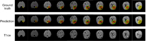
The proposed model has attained better results with transfer learning approach after implementing it with dropout layer. The prediction for the segmented tumor images has been accurately segmented. Figure 9 shows the difference between automatic segmentation and the actual ground values. From Figure 9, it is clearly predicted that the quality of the images has been enhanced as position, outline and size of the tumor has been accurately predicted. The proposed algorithm has shown better quantitative results such as dice score coefficient (DSC) for all three categories of tumor.
Below Table 4 provides information about different evaluators such as dice score, mean square error, peak signal to noise ratio, and similarity index. From the dataset of 150 images, some of the best segmentation results are elaborated in the Table 4. The dice score of second image is 0.910 and eighth image is 0.920. The dice score values of all the images have been upgraded by introducing the dropout layer in transfer learning model and segmentation model.
Figure 9. Ground Truth vs automated segmentation
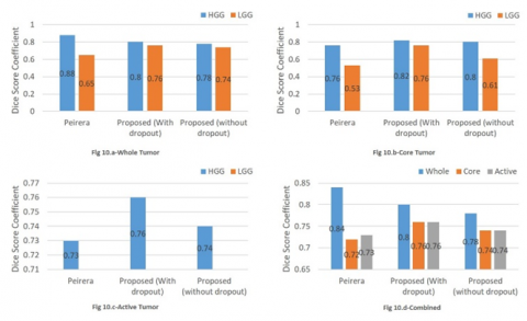
Figure 10. Comparative analysis of proposed model (with and without dropout layer)
Table 4. Parameters for segmented tissues and its performance analysis (with dropout)
|
Images |
MSE |
PSNR |
SSIM |
DSC |
|
Img1 |
1.957 |
56.45 dB |
0.8949 |
0.840 |
|
Img2 |
0.710 |
68.91 dB |
0.9190 |
0.910 |
|
Img3 |
3.920 |
58.12 dB |
0.9758 |
0.875 |
|
Img4 |
4.190 |
57.61 dB |
0.8286 |
0.880 |
|
Img5 |
1.410 |
55.64 dB |
0.8720 |
0.800 |
|
Img6 |
2.720 |
58.25dB |
0.9655 |
0.840 |
|
Img7 |
4.240 |
61.59 dB |
0.8190 |
0.890 |
|
Img8 |
0.410 |
50.61dB |
0.8290 |
0.920 |
|
Img9 |
1.210 |
51.61dB |
0.8128 |
0.895 |
|
Img10 |
1.091 |
52.45dB |
0.9112 |
0.900 |
|
Img11 |
3.021 |
52.67dB |
0.9234 |
0.909 |
A comparison of the proposed model with dropout and without dropout along with the deep learning method for Pereira et al. [50] is shown in the Figure 10. The segmentation results are quantified based on dice score coefficient value. In this figure, dice coefficient values of low-grade gliomas and high-grade gliomas are calculated in three categories of tumor (whole tumor, core tumor and active tumor) along with various parametric sets both of high-grade and low-grade gliomas. Figure 10.a represents the comparative analysis between Pereira’s model, proposed model (with and without dropout) for whole tumor. Figure 10.b represents comparison between the mentioned models for core tumor. The low-grade gliomas are usually not in active tumor state due to which their value is 0.00 in the Figure 10.c. Figure 10.d represents the overall performance of the three models for WT, CT and AT. HGG and LGG in whole tumor has DSC 0.80 and 0.76 with dropout. The HGG and LGG in core tumor has DSC 0.82 and 0.76 with dropout hence enhancing the segmentation results.
This research work aims in identifying a general, precise and robust segmentation algorithm for real time automatic segmentation of brain tumors solving all real world problems such as limited training data, noisy inputs and poor interactions within healthy and unhealthy tissues. For designing of automatic segmentation algorithm, research has been inspired from transfer learning model, energy function in deep convolutional neural network (DCNN), benefits of dropout layer, patch extraction from images for detecting brain tumors and accurately segmenting the brain tumor. The transfer learning approach when merged with the dropout layer has resulted in excellent segmentation results both in qualitative and quantitative manner. The algorithms are encapsulated together in a single framework to perform the task of brain tumor segmentation. The proposed model consists of 11-layered capsulated deep convolutional neural network that incorporates transfer learning model and segmentation model. Both the models have utilized dropout function with different dropout rate. The proposed architecture has maintained the simplicity in computational architecture for convolutional neural network (CNN). In this research paper, we have revised, implemented and observed the segmentation process of tumor from MR images and trained the CNN to perform automatic segmentation. Due to the transfer learning with dropout, the model has achieved high dice score coefficient such as 0.80 in WT (whole tumor), 0.76 in CT (core tumor) and 0.76 in AT (active tumor).
This research has focused on improving the efficiency of segmentation results by adding the transfer-learning model to the deep convolutional neural network (DCNN). This research enhances the segmentation results both in qualitative and quantitative manner. Qualitative measures such as accuracy, sensitivity, precision are considered using the quantitative measures such as similarity index, mean square error and peak signal to noise ratio evaluated for the complete dataset. This research is focused on implementing an algorithm for augmenting the computational speed and adaptability of the existing automatic brain tumor segmentation algorithms.
We acknowledge that this research is original and nowhere submitted, and there is no conflict of interest between authors and we have not received any funds for this research.
|
SSIM |
Structural Similarity Index |
|
DSC |
Dice Score Coefficient |
|
PSNR |
Peak Signal to Noise Ratio |
|
MSE |
Mean square error |
|
MRI |
Magnetic Resonance Imaging |
|
CNN |
Convolutional Neural Networks |
|
DBN |
Deep Belief Networks |
|
RBM |
Restricted Boltzmann’s Machine |
|
SAE |
Stacked Auto-encoders |
|
CT |
Core Tumor |
|
WT |
Whole Tumor |
|
AT |
Active Tumor |
|
HGG |
High Grade Gliomas |
|
LGG |
Low Grade Gliomas |
|
FCNN |
Fully Convolutional Neural Network |
[1] Huang, G., Huang, G.B., Song, S., You, K. (2015). Trends in extreme learning machines: A review. Neural Networks, 61: 32-48. https://doi.org/10.1016/j.neunet.2014.10.001
[2] Nyúl, L.G., Udupa, J.K., Zhang, X. (2000). New variants of a method of MRI scale standardization. IEEE Transactions on Medical Imaging, 19(2): 143-150. https://doi.org/10.1109/42.836373
[3] Ramesh, N., Yoo, J.H., Sethi, I.K. (1995). Thresholding based on histogram approximation. IEE Proceedings-Vision, Image and Signal Processing, 142(5): 271-279. https://doi.org/10.1049/ip-vis:19952007
[4] Dridi, M., Bouallegue, B., Hajjaji, M.A., Mtibaa, A. (2016). An enhencment medical image compression algorithm based on neural network. International Journal of Advanced Computer Science and Applications, 7(5): 484-489. https://doi.org/10.14569/IJACSA.2016.070565
[5] Trinh, D.H., Luong, M., Dibos, F., Rocchisani, J.M., Pham, C.D., Nguyen, T.Q. (2014). Novel example-based method for super-resolution and denoising of medical images. IEEE Transactions on Image Processing, 23(4): 1882-1895. https://doi.org/10.1109/TIP.2014.2308422
[6] Demirhan, A., Törü, M., Güler, I. (2014). Segmentation of tumor and edema along with healthy tissues of brain using wavelets and neural networks. IEEE Journal of Biomedical and Health Informatics, 19(4): 1451-1458. https://doi.org/10.1109/JBHI.2014.2360515
[7] Yasmin, M., Sharif, M., Mohsin, S. (2013). Neural networks in medical imaging applications: A survey. World Applied Sciences Journal, 22(1): 85-96. https://doi.org/10.5829/idosi.wasj.2013.22.01.72188
[8] Pham, D.L., Prince, J.L. (1999). Adaptive fuzzy segmentation of magnetic resonance images. IEEE Transactions on Medical Imaging, 18(9): 737-752. https://doi.org/10.1109/42.802752
[9] Prajapati, D.G., Sheth, K.R. (2017). Super-resolution technique for mri images using artificial neural network. International Journal on Recent and Innovation Trends in Computing and Communication, 5(4): 55-58. https://doi.org/10.17762/ijritcc.v5i4.360
[10] Zhao, J., Meng, Z., Wei, L., Sun, C., Zou, Q., Su, R. (2019). Supervised brain tumor segmentation based on gradient and context-sensitive features. Frontiers in neuroscience, 13: 144. https://doi.org/10.3389/fnins.2019.00144
[11] Coatrieux, G., Huang, H., Shu, H., Luo, L., Roux, C. (2013). A watermarking-based medical image integrity control system and an image moment signature for tampering characterization. IEEE Journal of Biomedical and Health Informatics, 17(6): 1057-1067. https://doi.org/10.1109/JBHI.2013.2263533
[12] Kong, Y., Deng, Y., Dai, Q. (2014). Discriminative clustering and feature selection for brain MRI segmentation. IEEE Signal Processing Letters, 22(5): 573-577. https://doi.org/10.1109/LSP.2014.2364612
[13] Saudagar, A.K.J. (2014). Minimize the percentage of noise in biomedical images using neural networks. The Scientific World Journal, 2014. https://doi.org/10.1155/2014/757146
[14] Mehdy, M.M., Ng, P.Y., Shair, E.F., Saleh, N.I., Gomes, C. (2017). Artificial neural networks in image processing for early detection of breast cancer. Computational and Mathematical Methods in Medicine, 2017: 2610628. https://doi.org/10.1155/2017/2610628
[15] Noh, H., Hong, S., Han, B. (2015). Learning deconvolution network for semantic segmentation. In Proceedings of the IEEE International Conference on Computer Vision, pp. 1520-1528.
[16] Dridi, M., Bouallegue, B., Hajjaji, M.A., Mtibaa, A. (2016). An enhencment medical image compression algorithm based on neural network. International Journal of Advanced Computer Science and Applications, 7(5): 484-489. https://doi.org/10.14569/IJACSA.2016.070565
[17] Arel, I., Rose, D.C., Karnowski, T.P. (2010). Deep machine learning-a new frontier in artificial intelligence research [research frontier]. IEEE Computational Intelligence Magazine, 5(4): 13-18. https://doi.org/10.1109/MCI.2010.938364
[18] Isa, I.S., Sulaiman, S.N., Mustapha, M., Karim, N.K.A. (2017). Automatic contrast enhancement of brain MR images using Average Intensity Replacement based on Adaptive Histogram Equalization (AIR-AHE). Biocybernetics and Biomedical Engineering, 37(1): 24-34. https://doi.org/10.1016/j.bbe.2016.12.003
[19] Demirhan, A., Törü, M., Güler, I. (2014). Segmentation of tumor and edema along with healthy tissues of brain using wavelets and neural networks. IEEE Journal of Biomedical and Health Informatics, 19(4): 1451-1458. https://doi.org/10.1109/JBHI.2014.2360515
[20] Benson, C.C., Lajish, V.L. (2014). Morphology based enhancement and skull stripping of MRI brain images. In 2014 International Conference on Intelligent Computing Applications, Coimbatore, India, pp. 254-257. https://doi.org/10.1109/ICICA.2014.61
[21] Tustison, N.J., Avants, B.B., Cook, P.A., Zheng, Y., Egan, A., Yushkevich, P.A., Gee, J.C. (2010). N4ITK: improved N3 bias correction. IEEE Transactions on Medical Imaging, 29(6): 1310-1320. https://doi.org/10.1109/TMI.2010.2046908
[22] Schmidhuber, J. (2015). Deep learning in neural networks: An overview. Neural Networks, 61: 85-117. https://doi.org/10.1016/j.neunet.2014.09.003
[23] Bharati, S., Podder, P., Mondal, M.R.H. (2020). Artificial neural network based breast cancer screening: a comprehensive review. International Journal of Computer Information Systems and Industrial Management Applications, 12(2020): 125-137.
[24] Vincent, P., Larochelle, H., Lajoie, I., Bengio, Y., Manzagol, P.A., Bottou, L. (2010). Stacked denoising autoencoders: Learning useful representations in a deep network with a local denoising criterion. Journal of Machine Learning Research, 11(12): 3371-3408.
[25] Hinton, G.E., Osindero, S., Teh, Y.W. (2006). A fast learning algorithm for deep belief nets. Neural Computation, 18(7): 1527-1554. https://doi.org/10.1162/neco.2006.18.7.1527
[26] Elleuch, M., Kherallah, M. (2020). Off-line Handwritten Arabic text recognition using convolutional DL networks. International Journal of Computer Information Systems and Industrial Management Applications, 12: 104-112.
[27] Bengio, Y., Lamblin, P., Popovici, D., Larochelle, H. (2007). Greedy layer-wise training of deep networks. In Advances in Neural Information Processing Systems, 153-160.
[28] Choi, H., Jin, K.H. (2016). Fast and robust segmentation of the striatum using deep convolutional neural networks. Journal of Neuroscience Methods, 274: 146-153. https://doi.org/10.1016/j.jneumeth.2016.10.007
[29] Zhang, W., Li, R., Deng, H., Wang, L., Lin, W., Ji, S., Shen, D. (2015). Deep convolutional neural networks for multi-modality isointense infant brain image segmentation. NeuroImage, 108: 214-224. https://doi.org/10.1016/j.neuroimage.2014.12.061
[30] Bao, S., Chung, A.C. (2018). Multi-scale structured CNN with label consistency for brain MR image segmentation. Computer Methods in Biomechanics and Biomedical Engineering: Imaging & Visualization, 6(1): 113-117. https://doi.org/10.1080/21681163.2016.1182072
[31] Chen, H., Dou, Q., Yu, L., Qin, J., Heng, P.A. (2018). VoxResNet: Deep voxelwise residual networks for brain segmentation from 3D MR images. NeuroImage, 170: 446-455. https://doi.org/10.1016/j.neuroimage.2017.04.041
[32] Ghafoorian, M., Karssemeijer, N., Heskes, T., Bergkamp, M., Wissink, J., Obels, J., Platel, B. (2017). Deep multi-scale location-aware 3D convolutional neural networks for automated detection of lacunes of presumed vascular origin. NeuroImage: Clinical, 14: 391-399. https://doi.org/10.1016/j.nicl.2017.01.033
[33] Ghafoorian, M., Karssemeijer, N., Heskes, T., van Uden, I.W., Sanchez, C.I., Litjens, G., Platel, B. (2017). Location sensitive deep convolutional neural networks for segmentation of white matter hyperintensities. Scientific Reports, 7(1): 1-12. https://doi.org/10.1038/s41598-017-05300-5
[34] Kleesiek, J., Urban, G., Hubert, A., Schwarz, D., Maier-Hein, K., Bendszus, M., Biller, A. (2016). Deep MRI brain extraction: A 3D convolutional neural network for skull stripping. NeuroImage, 129: 460-469. https://doi.org/10.1016/j.neuroimage.2016.01.024
[35] Milletari, F., Navab, N., Ahmadi, S.A. (2016). V-net: Fully convolutional neural networks for volumetric medical image segmentation. In 2016 Fourth International Conference on 3D Vision (3DV), pp. 565-571. https://doi.org/10.1109/3DV.2016.79
[36] Milletari, F., Ahmadi, S.A., Kroll, C., Plate, A., Rozanski, V., Maiostre, J., Navab, N. (2017). Hough-CNN: deep learning for segmentation of deep brain regions in MRI and ultrasound. Computer Vision and Image Understanding, 164: 92-102. https://doi.org/10.1016/j.cviu.2017.04.002
[37] Moeskops, P., Viergever, M.A., Mendrik, A.M., De Vries, L.S., Benders, M.J., Išgum, I. (2016). Automatic segmentation of MR brain images with a convolutional neural network. IEEE Transactions on Medical Imaging, 35(5): 1252-1261. https://doi.org/10.1109/TMI.2016.2548501
[38] Shakeri, M., Tsogkas, S., Ferrante, E., Lippe, S., Kadoury, S., Paragios, N., Kokkinos, I. (2016). Sub-cortical brain structure segmentation using F-CNN's. In 2016 IEEE 13th International Symposium on Biomedical Imaging (ISBI), pp. 269-272. https://doi.org/10.1109/ISBI.2016.7493261
[39] Zhao, L., Jia, K. (2016). Multiscale CNNs for brain tumor segmentation and diagnosis. Computational and Mathematical Methods in Medicine, 2016: 8356294. https://doi.org/10.1155/2016/8356294
[40] Pan, Y., Huang, W., Lin, Z., Zhu, W., Zhou, J., Wong, J., Ding, Z. (2015). Brain tumor grading based on neural networks and convolutional neural networks. In 2015 37th Annual International Conference of the IEEE Engineering in Medicine and Biology Society (EMBC), pp. 699-702. https://doi.org/10.1109/EMBC.2015.7318458
[41] Dou, Q., Chen, H., Yu, L., Shi, L., Wang, D., Mok, V.C., Heng, P.A. (2015). Automatic cerebral microbleeds detection from MR images via independent subspace analysis based hierarchical features. In 2015 37th Annual International Conference of the IEEE Engineering in Medicine and Biology Society (EMBC), pp. 7933-7936. https://doi.org/10.1109/EMBC.2015.7320232
[42] Dou, Q., Chen, H., Yu, L., Zhao, L., Qin, J., Wang, D., Heng, P.A. (2016). Automatic detection of cerebral microbleeds from MR images via 3D convolutional neural networks. IEEE Transactions on Medical Imaging, 35(5): 1182-1195. https://doi.org/10.1109/TMI.2016.2528129
[43] de Brebisson, A., Montana, G. (2015). Deep neural networks for anatomical brain segmentation. In Proceedings of the IEEE Conference on Computer Vision and Pattern Recognition Workshops, pp. 20-28.
[44] Navab, N., Hornegger, J., Wells, W.M., Frangi, A. (2015). Medical image computing and computer-assisted intervention. MICCAI 2015: 18th International Conference, Munich, Germany, Proceedings, Part III, 9351: 3-4.
[45] Kamnitsas, K., Chen, L., Ledig, C., Rueckert, D., Glocker, B. (2015). Multi-scale 3D convolutional neural networks for lesion segmentation in brain MRI. Ischemic Stroke Lesion Segmentation, 13: 46.
[46] Paulsen, R.R., Pedersen, K.S. (2015). Image Analysis. 19th Scandinavian Conference, SCIA 2015, Copenhagen, Denmark, June 15-17, 2015. Proceedings, 9127.
[47] Hu, K., Gan, Q., Zhang, Y., Deng, S., Xiao, F., Huang, W., Gao, X. (2019). Brain tumor segmentation using multi-cascaded convolutional neural networks and conditional random field. IEEE Access, 7: 92615-92629. https://doi.org/10.1109/ACCESS.2019.2927433
[48] Isensee, F., Maier-Hein, K.H. (2021). nnU-Net for Brain Tumor Segmentation. In Brainlesion: Glioma, Multiple Sclerosis, Stroke and Traumatic Brain Injuries: 6th International Workshop, BrainLes 2020, Held in Conjunction with MICCAI 2020, Lima, Peru, October 4, 2020, Revised Selected Papers, Part II, 12658: 118. https://doi.org/10.1007/978-3-030-72087-2_11
[49] Yousefi, S., Sokooti, H., Elmahdy, M.S., Lips, I.M., Shalmani, M.T.M., Zinkstok, R.T., Staring, M. (2020). Esophageal Tumor Segmentation in CT Images using Dilated Dense Attention Unet (DDAUnet). arXiv preprint arXiv:2012.03242.
[50] Shen, L., Anderson, T. (2017). Multimodal brain MRI tumor segmentation via convolutional neural networks. http://cs231n.stanford.edu/reports/2017/pdfs/512.pdf.
[51] Xiang, C., Zhang, L., Tang, Y., Zou, W., Xu, C. (2018). MS-CapsNet: A novel multi-scale capsule network. IEEE Signal Processing Letters, 25(12): 1850-1854. https://doi.org/10.1109/LSP.2018.2873892
[52] Bhardwaj, S., Pandove, G., Dahiya, P.K. (2020). A futuristic hybrid image retrieval system based on an effective indexing approach for swift image retrieval. International Journal of Computer Information Systems and Industrial Management Applications, 12: 1-13.
[53] Pereira, S., Pinto, A., Alves, V., Silva, C.A. (2016). Brain tumor segmentation using convolutional neural networks in MRI images. IEEE Transactions on Medical Imaging, 35(5): 1240-1251. https://doi.org/10.1109/TMI.2016.2538465
[54] Chen, C.M., Chen, C.C., Wu, M.C., Horng, G., Wu, H.C., Hsueh, S.H., Ho, H.Y. (2015). Automatic contrast enhancement of brain MR images using hierarchical correlation histogram analysis. Journal of Medical and Biological Engineering, 35(6): 724-734. https://doi.org/10.1007/s40846-015-0096-6
[55] Purkait, P., Chanda, B. (2012). Super resolution image reconstruction through Bregman iteration using morphologic regularization. IEEE Transactions on Image Processing, 21(9): 4029-4039. https://doi.org/10.1109/TIP.2012.2201492
[56] Yang, J., Wang, Z., Lin, Z., Cohen, S., Huang, T. (2012). Coupled dictionary training for image super-resolution. IEEE Transactions on Image Processing, 21(8): 3467-3478. https://doi.org/10.1109/TIP.2012.2192127
[57] Shi, Z., He, L., Suzuki, K., Nakamura, T., Itoh, H. (2009). Survey on neural networks used for medical image processing. International Journal of Computational Science, 3(1): 86.
[58] Wang, H., Roa, A.C., Basavanhally, A.N., Gilmore, H.L., Shih, N., Feldman, M., Madabhushi, A. (2014). Mitosis detection in breast cancer pathology images by combining handcrafted and convolutional neural network features. Journal of Medical Imaging, 1(3): 034003. https://doi.org/10.1117/1.JMI.1.3.034003
[59] Yadav, S.S., Jadhav, S.M. (2019). Deep convolutional neural network based medical image classification for disease diagnosis. Journal of Big Data, 6(1): 1-18. https://doi.org/10.1186/s40537-019-0276-2
[60] Okuhata, H., Imai, R., Ise, M., Omaki, R.Y., Nakamura, H., Hara, S., Shirakawa, I. (2014). Implementation of dynamic-range enhancement and super-resolution algorithms for medical image processing. In 2014 IEEE International Conference on Consumer Electronics (ICCE), pp. 181-184. https://doi.org/10.1109/ICCE.2014.6775963
[61] Sharma, N., Aggarwal, L.M. (2010). Automated medical image segmentation techniques. Journal of medical physics/Association of Medical Physicists of India, 35(1): 3. https://doi.org/10.4103/0971-6203.58777
[62] Lai, M. (2015). Deep learning for medical image segmentation. arXiv preprint arXiv:1505.02000.
[63] Da, C., Zhang, H., Sang, Y. (2015). Brain CT image classification with deep neural networks. In Proceedings of the 18th Asia Pacific Symposium on Intelligent and Evolutionary Systems, 1: 653-662. https://doi.org/10.1007/978-3-319-13359-1_50
[64] Kansal, T., Bahuguna, S., Singh, V., Choudhury, T. (2018). Customer segmentation using K-means clustering. In: 2018 International Conference on Computational Techniques, Electronics and Mechanical Systems (CTEMS).
[65] Verma, A., Tripathi, A., Choudhury, T. (2020). Implementing brain-machine interface (BMI) with smart computing. Computational Intelligence in Pattern Recognition, Springer, Singapore, pp. 71-81. https://doi.org/10.1007/978-981-15-2449-3_5