Sanaz Moezzi| Mehrdad Jalali | Yahya Forghani*
OPEN ACCESS
Based on twin support vector machines (TWSVM) model, the twin support vector clustering (TWSVC) is a planar clustering model that increases inter-cluster separation. Because the TWSVC is not a standard model for some variables, its solving algorithm consumes lots of time and does not always converge to the optimal solution. To solve the problem, this paper proposes a novel clustering model, denoted as TWSVC+, based on twin support vector machines (TWSVM). The TWSVC+ is convex and standard with respect to each variable. Therefore, it is possible to solve this model rapidly with an algorithm that converges to a global optimal solution relative to each variable. The author presented linear TWSVC+ and non-linear TWSVC+ for clustering linear separable clusters and linear inseparable clusters, respectively. Experimental results on real datasets of UCI repository show that the TWSVC+ was better than TWSVC and support vector clustering (SVC) in accuracy and training time.
plane-based clustering, support vector clustering (SVC), twin support vector clustering (TWSVC), convex
Clustering is a main procedure for data mining with wide application such as community detection, image processing, gene analysis, text organization, etc. K-Means and its extensions [1-5] are one class of the most famous clustering models. K-Means extracts clusters such that the data of each cluster have minimum distance to its cluster center which is a point. Hence, k-means is a point-based clustering model which tries to increase intra-cluster compactness. Other main category of clustering models are plane-based clustering models, e.g. k-plane clustering (kPC) [6, 7], proximal plane clustering (PPC) [8, 9], support vector clustering (SVC) [10, 11] and twin support vector clustering (TWSVC) [12]. In plane-based clustering model, cluster center or cluster boundary is a plane. SVC [11] tries to increase inter-cluster separation. A faster version of SVC was proposed by K. Zhang, et al. [10]. Their experimental results show that the accuracy of SVC is higher than K-Means. But, when the number of data increases, memory-usage and training time of SVC increases dramatically. SVC is based on a well-known classification model named support vector machine (SVM) [13]. Training time and accuracy of Twin SVM (TWSVM) [14-16] are better than those of SVM. The existing TWSVM-based clustering, i.e. TWSVC [12], is not a standard model with respect to some of its variables. Therefore, a time-consuming algorithm named concave-convex algorithm [17] is used to solve TWSVC with respect to the mentioned variables. Moreover, the concave-convex algorithm does not guarantee a global optimal solution with respect to the mentioned variables.
This paper proposes a novel TWSVM-based clustering model called TWSVC+, which is convex and standard with respect to each model variable. Therefore, there is a fast algorithm for solving TWSVC+ with respect to each model variable which guarantees a global optimal solution of TWSVC+ with respect to each model variable. For simplicity, it assumed that we are dealing with two-cluster clustering. Therefore, the proposed model is explained based on a two-cluster TWSVM: Assuming that we have only two clusters, initial clustering is done by using k-Means and therefore, the membership degrees of data to each initial cluster are determined. Then, cluster centers are corrected using TWSVM because data labels or data membership degrees were determined, previously. Next, data labels are corrected according to cluster centers learned using TWSVM. The process of correcting cluster centers and data labels is continued until convergence. Our experiments on the real dataset of UCI repository, i.e. Sonar, Cancer, PID, Iris and Wine show that the accuracy of TWSVC+ is better than that of k-means, SVC and TWSVC, and the training time of TWSVC+ is less than that of TWSVC and SVC.
In continue, in section 2, TWSVC is explained. As our proposed clustering model is based on TWSVM, it is briefly explained in section 2, too. In section 3, TWSVC+ is proposed. In section 4, TWSVC+ is evaluated using real dataset and in section 5, the conclusion is provided.
2.1 TWSVC for clustering
Let $\mathrm{X}=\left\{\mathrm{x}_{1}, \mathrm{x}_{2}, \ldots, \mathrm{x}_{\mathrm{N}}\right\}$ be data which must be clustered into k clusters where $\forall \mathrm{i}: \mathrm{x}_{\mathrm{i}} \in \mathrm{R}^{\mathrm{m}}$. TWSVC [6] assumes that the center of i-th cluster is a hyperplane with the equation $\mathrm{w}_{\mathrm{i}}^{\mathrm{T}} \mathrm{x}+\mathrm{b}_{\mathrm{i}}=0$, where $w_{i}$ is the weight vector and $b_{i}$ is the bias of the mentioned hyperplane. TWSVM finds i-th cluster center or i-th hyperplane such that members of this cluster are in the vicinity of i-th hyperplane and members of other clusters, are away from this hyperplane. For this purpose, the following mathematical model is used:
$\min _{\mathbf{w}_{\mathbf{i}}, \mathbf{b}_{\mathbf{i}}, \mathbf{q}_{\mathbf{i}}} \frac{1}{2}\left\|{X}_{{i}} {w}_{{i}}+{b}_{{i}} {e}\right\|^{2}+{c} \tilde{{e}}^{{T}} {q}_{{i}}$
subject to $\left|\widetilde{X}_{{i}} w_{{i}}+{b}_{{i}} \tilde{{e}}\right| \geq \tilde{{e}}-{q}_{{i}} ; {q}_{{i}} \geq 0$ (1)
where, $\mathrm{i}=1,2, \ldots, \mathrm{k}$; $\mathrm{X}_{\mathrm{i}}$ is i-th data cluster and $\widetilde{\mathrm{X}}_{\mathrm{i}}$ is the other data clusters located on both sides of the i-th cluster center. The term $\left\|\mathrm{X}_{\mathrm{i}} \mathrm{w}_{\mathrm{i}}+\mathrm{b}_{\mathrm{i}} \mathrm{e}\right\|^{2}$ of the model objective function (1) minimize the Euclidean distance of i-th cluster data to i-th cluster center. $q_{i}$ is slack vector which exceptionally allows some data of $\widetilde{\mathrm{X}}_{\mathrm{i}}$ not to be far enough from the i-th cluster center. These data are called outliers. Each of e and $\tilde{\mathrm{e}}$ are vectors whose elements are equal to 1. The parameter $c \geq 0$ determines the importance of the second term of the model objective function (1) compared to its first term. If the value of c is large, less number of $\widetilde{\mathrm{X}}_{\mathrm{i}}$ are allowed not to be far enough from i-th cluster center. Instead, it is possible that i-th cluster data, i.e. $\mathrm{X}_{\mathrm{i}}$, are not placed in the vicinity of i-th cluster center or i-th hyperplane. The model (1) is not a standard model because its first constraint is non-convex. The concave-convex algorithm which is a time-consuming algorithm is used to solve the model (1). Algorithm 1 [12] is an iterative algorithm which is used to solve the model (1) for clustering data into k cluster.
| Algorithm 1. An algorithm for solving TWSVC [12], i.e. the model (1). |
|
Input: $X=\left\{\mathrm{x}_{1}, \mathrm{x}_{2}, \ldots, \mathrm{x}_{\mathrm{N}}\right\}$ : Data k: The number of clusters. thr: a threshold. Output: k cluster centers. |
|
2.2 TWSVM for two class classification
$\min _{\mathbf{w}, \mathbf{b}, \mathbf{q}} \frac{1}{2}\|\mathrm{Xw}+\mathrm{b} \tilde{\mathrm{e}}\|^{2}+\mathrm{ce}^{\mathrm{T}} \mathrm{q}$
subject to $-(\widetilde{\mathrm{X}} \mathrm{w}+\mathrm{be}) \geq \mathrm{e}-\mathrm{q} ; \mathrm{q} \geq 0$ (2)
$\min _{\widetilde{\mathbf{w}}, \tilde{\mathbf{b}}, \tilde{\mathbf{q}}} \frac{1}{2}\|\widetilde{{X}} \widetilde{{w}}+\widetilde{{b}} e\|^{2}+\tilde{{c}} \tilde{e}^{\mathrm{T}} \tilde{{q}}$
subject to $(\mathrm{X} \widetilde{\mathrm{w}}+\widetilde{\mathrm{b}} \tilde{e}) \geq \tilde{e}-\tilde{{q}} ; \tilde{{q}} \geq 0$ (3)
where, $\mathrm{w}^{\mathrm{T}} \mathrm{x}+\mathrm{b}=0$ and $\widetilde{\mathbf{w}}^{\mathrm{T}} \mathbf{x}+\widetilde{\mathbf{b}}=0$ are the borders or the center of each of the two data classes, and w and b are the weight vector and the bias of the first class center, and w and b are the weight vector $\widetilde{\mathbf{w}}$ and $\widetilde{\mathrm{b}}$ the bias of the second class center. X is the first data class and $\widetilde{\mathrm{X}}$ is the second data class. The term $\|\mathrm{Xw}+\mathrm{b} \tilde{e}\|^{2}$ in the objective function of the model (2), minimizes Euclidean distance of the first data class from the first class center. The vector q is slack vector which allows some of the second data class not to be far enough from the first class center. Such data are called outliers. Each of e and $\tilde{\mathrm{e}}$ is a vector whose elements are equal to 1. The parameter $c \geq 0$ determines the importance of the second term of the objective function (2) compared to its first term. If the value of c is large, less number of the second data class are allowed not to be far enough from the first cluster center. Instead, it is possible that the first data class is not placed in the vicinity of the first class center. The parameter c controls the generalization ability of classifier which can increase the classifier accuracy.
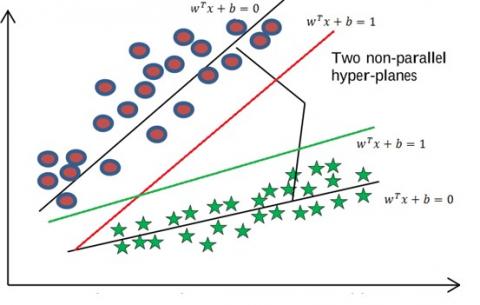
The term $\|\widetilde{\mathrm{X}} \widetilde{\mathrm{w}}+\widetilde{\mathrm{b}} e\|^{2}$ in the objective function of the model (3), minimizes Euclidean distance of the second data class from the second class center. The vector $\tilde{q}$ is slack vector which allows some of the first data class not to be far enough from the second class center. Such data are called outliers. The parameter $\tilde{c} \geq 0$ determines the importance of the second term of the objective function (3) compared to its first term. If the value of c is large, less number of the first data class are allowed not to be far enough from the second cluster center. Instead, it is possible that the second data class is not placed in the vicinity of the second class center. Figure 1 shows how TWSVM classifies data.
Figure 1. Classification of data using TWSVM
As it was mentioned, the existing TWSVC is not a standard model with respect to some of its variables. Therefore, a time-consuming algorithm named concave-convex algorithm is used to solve TWSVC with respect to the mentioned variables. Moreover, the concave-convex algorithm does not guarantee a global optimal solution with respect to the mentioned variables. In this section, we propose a novel TWSVM-based clustering model called TWSVC+, which is convex and standard with respect to each model variable. Therefore, there is fast algorithm for solving TWSVC+ with respect to each model variable which guarantees a global optimal solution of TWSVC+ with respect to each model variable.
In two following sub-sections, linear TWSVC+ and non-linear TWSVC+ is presented for clustering linear separable clusters and linear inseparable clusters, respectively.
3.1 Linear TWSVC+
TWSVC+ is based on the basic TWSVM. The basic TWSVM is a two-class classifier which learns a classifier based on a two-class training data. One can design a multi-class classifier by using some two-class TWSVM models, e.g. DAG approach. In this paper, for simplicity, it is assumed that we want to cluster data into two clusters. Therefore, the proposed model is described based on a two-class TWSVM. Obviously, similarly, by combining several two-cluster clustering model, we can create a multi-cluster clustering model.
Suppose that we want to group $\left\{\mathrm{x}_{1}, \mathrm{x}_{2}, \dots, \mathrm{x}_{\mathrm{N}}\right\}$ into two clusters n and p. Initialize cluster centers and data membership degree $\mathrm{U}_{\mathrm{ip}} \in\{0,1\}$ and $\mathrm{U}_{\mathrm{in}} \in\{0,1\}$, i.e. membership degree of $\mathrm{x}_{\mathrm{i}}$ to clusters p and n, respectively, by using k-means or randomly. Then, cluster centers can be determined using TWSVM model because data labels or data membership degrees were determined, previously. To be more precise, to determine the two cluster centers, it is enough to solve the following twin models:
$\min _{\mathbf{w} ‘ \mathbf{b} ‘ \mathbf{q}} \sum_{\mathbf{i}=1}^{\mathrm{N}}\left(\mathbf{w}^{\mathrm{T}} \mathbf{x}_{\mathbf{i}}+\mathbf{b}\right)^{2} \mathrm{U}_{\mathrm{ip}}+\mathrm{c} \sum_{\mathrm{i}=1}^{\mathrm{N}} \mathrm{q}_{\mathrm{i}} \mathrm{U}_{\mathrm{in}}$
subject to $\left\{\begin{array}{l}{-\left(\mathrm{w}^{\mathrm{T}} \mathrm{x}_{\mathrm{i}}+\mathrm{b}\right) \geq 1-\mathrm{q}_{\mathrm{i}}} \\ {\mathrm{q}_{\mathrm{i}} \geq 0, \mathrm{i}=1,2, \ldots, \mathrm{N}}\end{array}\right.$ (4)
$\min _{\tilde{\mathbf{W}} ‘ \tilde{\mathbf{b}} ‘ \tilde{\mathbf{q}}} \sum_{\mathrm{i}=1}^{\mathrm{N}}\left(\widetilde{\mathbf{w}}^{\mathrm{T}} \mathbf{x}_{\mathrm{i}}+\tilde{\mathrm{b}}\right)^{2} \mathrm{U}_{\mathrm{in}}+\tilde{\mathrm{c}} \sum_{\mathrm{i}=1}^{\mathrm{N}} \tilde{\mathrm{q}}_{\mathrm{i}} \mathrm{U}_{\mathrm{ip}}$
subject to $\left\{\begin{array}{l}{\left(\widetilde{\mathrm{w}}^{\mathrm{T}} \mathrm{x}_{\mathrm{i}}+\tilde{\mathrm{b}}\right) \geq 1-\tilde{\mathrm{q}}_{\mathrm{i}}} \\ {\tilde{\mathrm{q}}_{\mathrm{i}} \geq 0, \quad \mathrm{i}=1,2, \ldots, \mathrm{N}}\end{array}\right.$ (5)
The first model, i.e. model (4), learns the center of cluster p or a hyperplane with the equation $\mathrm{w}^{\mathrm{T}} \mathrm{x}+\mathrm{b}=0$ such that the data of cluster n are located behind the hyperplane with an appropriate distance from it. In other word, for each x of the cluster n we must almost have $-\left(w^{T} x+b\right) \geq 1$, and for each x of the cluster p we must have $\mathrm{w}^{\mathrm{T}} \mathrm{x}+\mathrm{b}=0$ which is achieved by minimizing $\left(w^{T} x+b\right)^{2}$ in the model (4). The variable b is the bias and w is the weight vector of the center of cluster p. $\mathrm{q}_{\mathrm{i}}$ is slack variable which allows $\mathrm{x}_{\mathrm{i}}$ of the cluster n not to be in the proper distance behind the center of class p. Such data are called outliers. The parameter c controls the number of outliers of class n.
The second model, i.e. the model (5), learns the center of cluster n or a hyperplane with the equation $\widetilde{\mathbf{w}}^{\mathrm{T}} \mathbf{x}+\tilde{\mathbf{b}}=0$ such that the data of cluster p are located in front of the hyperplane with an appropriate distance from it. In other word, for each x of the cluster p we must almost have $\left(\widetilde{w}^{T} x_{i}+\tilde{b}\right) \geq 1$, and for each x of the cluster n we must have $\widetilde{\mathbf{w}}^{\mathrm{T}} \mathbf{x}+\tilde{\mathbf{b}}=0$ which is achieved by minimizing $\left(\widetilde{w}^{\mathrm{T}} x+\tilde{\mathrm{b}}\right)^{2}$ in the model (5). The variable $\tilde{\mathrm{b}}$ is the bias and $\widetilde{\mathbf{w}}$ is the weight vector of the center of cluster n. $\tilde{\mathrm{q}}_{\mathrm{i}}$ is slack variable which allows $\mathrm{x}_{\mathrm{i}}$ of the cluster p not to be in the proper distance in front of the center of class n. Such data is called outlier. Parameter c controls the number of outliers of class p.
Each of the models (4) and (5) is a standard model, i.e. Quadratic Programming Problem (QPP). There exist efficient and well-known algorithms to solve a QPP. Solving the duals of these two primal models, i.e. models (4) and (5), are faster than solving the primal models because their dual models has less variables and less constraints. Hence, in continue, the duals of each of these primal models is determined. The model (4) can be written as follows:
$\min _{\mathbf{w} ‘ \mathbf{b}‘ \mathbf{q}} \frac{1}{2}(\mathrm{Xw}+\mathrm{eb})^{\mathrm{T}} \operatorname{diag}\left(\mathrm{U}_{\mathrm{p}}\right)(\mathrm{Xw}+\mathrm{eb})+\mathrm{ce}^{\mathrm{T}}\left(\operatorname{diag}\left(\mathrm{U}_{\mathrm{n}}\right)\right) \mathrm{q}$
subject to $\left\{\begin{array}{l}{-(\mathrm{Xw}+\mathrm{eb}) \geq \mathrm{e}-\mathrm{q}} \\ {\mathrm{q} \geq 0}\end{array}\right.$ (6)
where, $\mathrm{X}=\left(\mathrm{x}_{1}, \mathrm{x}_{2}, \ldots, \mathrm{x}_{\mathrm{N}}\right)^{\mathrm{T}}$; $\mathrm{e} \in \mathrm{R}^{\mathrm{N}}$ is a vector whose elements are equal to 1; $\mathrm{U}_{\mathrm{p}}=\left(\mathrm{U}_{1 \mathrm{p}}, \mathrm{U}_{2 \mathrm{p}}, \ldots, \mathrm{U}_{\mathrm{Np}}\right)^{\mathrm{T}}$; $\mathrm{U}_{\mathrm{n}}=\left(\mathrm{U}_{1 \mathrm{n}}, \mathrm{U}_{2 \mathrm{n}}, \ldots, \mathrm{U}_{\mathrm{Nn}}\right)^{\mathrm{T}}$; and $\mathrm{q}=\left(\mathrm{q}_{1}, \mathrm{q}_{2}, \ldots, \mathrm{q}_{\mathrm{N}}\right)^{\mathrm{T}}$. The model (6) can be written as follows:
$\begin{aligned} \min _{\mathbf{w} ‘ \mathbf{b} ‘ \mathbf{q}} \frac{1}{2} \| \sqrt{\operatorname{diag}\left(\mathrm{U}_{\mathrm{p}}\right)} \mathrm{X} \mathrm{w}+& \sqrt{\operatorname{diag}\left(\mathrm{U}_{\mathrm{p}}\right)} \mathrm{eb} \|^{2} \\ &+\operatorname{ce}^{\mathrm{T}}\left(\operatorname{diag}\left(\mathrm{U}_{\mathrm{n}}\right)\right) \mathrm{q} \end{aligned}$
subject to $\left\{\begin{array}{l}{-(X w+e b) \geq e-q} \\ {q \geq 0}\end{array}\right.$ (7)
Let $\dot{\mathrm{x}}=\sqrt{\operatorname{diag}\left(\mathrm{U}_{\mathrm{p}}\right)} \mathrm{x}$, $\dot{\mathrm{e}}=\sqrt{\operatorname{diag}\left(\mathrm{U}_{\mathrm{p}}\right)}$, $\ddot{\mathrm{e}}=\operatorname{diag}\left(\mathrm{U}_{\mathrm{n}}\right) \mathrm{e}$ and $\operatorname{diag}\left(\mathrm{U}_{\mathrm{n}}\right)=\operatorname{diag}\left(1-\mathrm{U}_{\mathrm{p}}\right)$ Then, the model (7) can be rewritten as follows:
$\min _{\mathbf{w} ‘ \mathbf{b}‘ \mathbf{q}} \frac{1}{2}\|\dot{\mathbf{X}} \mathbf{w}+\dot{\mathbf{e}} \mathrm{b}\|^{2}+\mathrm{c} \ddot{\mathrm{e}}^{\mathrm{T}} \mathrm{q}$
subject to $\left\{\begin{array}{l}{-(X w+e b) \geq e-q} \\ {q \geq 0}\end{array}\right.$ (8)
Lagrange function of the model (8) is as follows:
$\mathcal{L}=\frac{1}{2}\|\dot{\mathrm{X}} \mathrm{w}+\dot{\mathrm{e}} \mathrm{b}\|^{2}+\mathrm{c} \ddot{\mathrm{e}}^{\mathrm{T}} \mathrm{q}-\alpha^{\mathrm{T}}(-(\mathrm{X} \mathrm{w}+\mathrm{eb})+\mathrm{q}-\mathrm{e})-\beta^{\mathrm{T}} \mathrm{q}$ (9)
where, $\alpha \geq 0$ and $\beta \geq 0$ are Lagrange coefficients. We have at the optimal point of the dual model:
$\frac{\mathrm{d} \mathcal{L}}{\mathrm{dw}}=0 \rightarrow \dot{\mathrm{X}}^{\mathrm{T}}(\dot{\mathrm{X}} \mathrm{w}+\dot{\mathrm{e}} \mathrm{b})+\mathrm{X}^{\mathrm{T}} \alpha=0$ (10)
$\frac{\mathrm{d} \mathcal{L}}{\mathrm{db}}=0 \rightarrow \dot{\mathrm{e}}^{\mathrm{T}}(\dot{\mathrm{X}} \mathrm{w}+\dot{\mathrm{e}} \mathrm{b})+\mathrm{e}^{\mathrm{T}} \alpha=0$ (11)
$\frac{\mathrm{d} \mathcal{L}}{\mathrm{dq}}=0 \rightarrow c\ddot{e}-\alpha-\beta=0$ (12)
According to Eq. (12) and given that $\beta \geq 0$ and $\alpha \geq 0$, we have:
$0 \leq \alpha \leq c\ddot{e}$ (13)
By combining Eq. (10) and Eq. (11) we obtain:
$\left[\dot{X}^{\mathrm{T}}, \dot{\mathrm{e}}^{\mathrm{T}}\right][\dot{\mathrm{X}}, \dot{\mathrm{e}}][\mathrm{w}, \mathrm{b}]+\left[\mathrm{X}^{\mathrm{T}}, \mathrm{e}^{\mathrm{T}}\right] \alpha=0$ (14)
We define $\mathrm{H}=\lceil\dot{\mathrm{X}}, \dot{\mathrm{e}}], \quad \mathrm{G}=[\mathrm{X}, \mathrm{e}]$ and $\mathrm{V}=[\mathrm{w}, \mathrm{b}]^{\mathrm{T}}$ Then, Eq. (14) can be written as follows:
$\mathrm{H}^{\mathrm{T}} \mathrm{HV}+\mathrm{G}^{\mathrm{T}} \alpha=0$ (15)
Therefore,
$\mathrm{V}=-\left(\mathrm{H}^{\mathrm{T}} \mathrm{H}\right)^{-1} \mathrm{G}^{\mathrm{T}} \alpha$ (16)
The matrix $\mathrm{H}^{\mathrm{T}} \mathrm{H}$ may be not invertible. In such situation, a small positive value $(\lambda)$ is added to its main diagonal. Then, we have:
$\mathrm{V}=-\left(\mathrm{H}^{\mathrm{T}} \mathrm{H}+\lambda \mathrm{I}\right)^{-1} \mathrm{G}^{\mathrm{T}} \alpha$ (17)
Moreover, by substituting Eq. (10)-(12) in the Lagrange function (9), the dual of the first model of the proposed twin models can be obtained as follows:
$\max _{\alpha}-\frac{1}{2} \alpha^{\mathrm{T}} G\left(\mathrm{H}^{\mathrm{T}} \mathrm{H}\right)^{-1} \mathrm{G}^{\mathrm{T}} \alpha+\mathrm{e}^{\mathrm{T}} \alpha$
subject to $0 \leq \alpha \leq c\ddot{e}$ (18)
By solving the model (18), and obtaining optimal $\alpha$ and putting it in Eq. (16) or Eq. (17), the value of V, i.e. the weight vector w and the bias b of center of cluster p, is obtained.
Similarly, by setting the gradient of Lagrange function of the second model of the proposed twin model, i.e. the model (5), equal to zero, we obtain:
$\widetilde{\nabla}=\left(\widetilde{\mathrm{H}}^{\mathrm{T}} \widetilde{\mathrm{H}}\right)^{-1} \mathrm{G}^{\mathrm{T}} \widetilde{\alpha}$ (19)
where, $\tilde{\alpha}$ is Lagrange coefficient; $\widetilde{\nabla}=[\widetilde{w} ‘ \tilde{\mathrm{b}}]^{\mathrm{T}} ; \widetilde{\mathrm{H}}=[\widetilde{\mathrm{X}}, \overline{\mathrm{e}}]$; $\widetilde{\mathrm{X}}=\sqrt{\operatorname{diag}\left(\mathrm{U}_{\mathrm{n}}\right)} \mathrm{X} ; \overline{\mathrm{e}}=\sqrt{\operatorname{diag}\left(\mathrm{U}_{\mathrm{n}}\right)} \mathrm{e}$; and $\overline{\overline{\mathrm{e}}}=\operatorname{diag}\left(\mathrm{U}_{\mathrm{p}}\right) \mathrm{e}$. Similarly, the dual of the model (5) can be obtained:
$\max _{\tilde{\alpha}}-\frac{1}{2} \widetilde{\alpha}^{\mathrm{T}} \widetilde{\mathrm{H}}\left(G^{\mathrm{T}} G\right)^{-1} \widetilde{\mathrm{H}}^{\mathrm{T}} \widetilde{\alpha}+\mathrm{e}^{\mathrm{T}} \widetilde{\alpha}$
subject to $\quad 0 \leq \widetilde{\alpha} \leq \tilde{\mathrm{c}}\overline{\overline{e}}$ (20)
By solving the model (20), and obtaining optimal $\widetilde{\alpha}$ and putting it in Eq. (19), the value of $\tilde{V}$, i.e. the weight vector $\widetilde{w}$ and the bias $\tilde{b}$ of center of class n, is obtained.
After determining the cluster centers using the models (18) and (20), the membership degrees of data to the clusters, or the values of $\mathrm{U}_{\mathrm{ip}}$ and $\mathrm{U}_{\mathrm{in}}$ must be modified such that the two clusters of data are as most distinctive as possible. That is, as far as possible, data of cluster p must be on the first hyperplane with the equation $\mathrm{w}^{\mathrm{T}} \mathrm{x}+\mathrm{b}=0$, namely $\sum_{i=1}^{N}\left(w^{T} x_{i}+b\right)^{2} U_{i p}$ must be minimized, while the data of cluster n must be located far behind the first hyperplane. Also, as far as possible, data of cluster n must be on the second hyperplane with the equation $\widetilde{\mathbf{w}}^{\mathrm{T}} \mathbf{x}+\tilde{\mathbf{b}}=0$, namely $\sum_{i=1}^{N}\left(\widetilde{W}^{T} X_{i}+\widetilde{b}\right)^{2} U_{i n}$ must be minimized, while the data of cluster p must be located far in front of the second hyperplane, and the number of clusters outliers must be reduced, or almost equivalently $\sum_{i=1}^{N} q_{i} U_{i n}$ and $\sum_{i=1}^{N} \widetilde{q}_{1} U_{i p}$ must be minimized. To this end, the following model is proposed:
$\begin{aligned} \min _{\mathbf{U}} & \sum_{\mathrm{i}=1}^{\mathrm{N}}\left(\mathrm{w}^{\mathrm{T}} \mathrm{x}_{\mathrm{i}}+\mathrm{b}\right)^{2} \mathrm{U}_{\mathrm{ip}}+\sum_{\mathrm{i}=1}^{\mathrm{N}} \mathrm{q}_{\mathrm{i}} \mathrm{U}_{\mathrm{in}} \\ &+\sum_{\mathrm{i}=1}^{\mathrm{N}}\left(\widetilde{\mathrm{w}}^{\mathrm{T}} \mathrm{x}_{\mathrm{i}}+\tilde{\mathrm{b}}\right)^{2} \mathrm{U}_{\mathrm{in}}+\sum_{\mathrm{i}=1}^{\mathrm{N}} \widetilde{\mathrm{q}}_{\mathrm{i} \mathrm{p}}U_{ip} \end{aligned}$
subject to $\left\{\begin{array}{l}{\mathrm{U}_{\mathrm{ip}}+\mathrm{U}_{\mathrm{in}}=1} \\ {\mathrm{U}_{\mathrm{ip}}, \mathrm{U}_{\mathrm{ip}} \in\{0,1\}, \mathrm{i}=1,2, \ldots, \mathrm{N}} \\ {-\mathrm{L} \leq \sum_{\mathrm{i}=1}^{\mathrm{N}} \mathrm{u}_{\mathrm{ip}}-\sum_{\mathrm{i}=1}^{\mathrm{N}} \mathrm{u}_{\mathrm{in}} \leq \mathrm{L}}\end{array}\right.$ (21)
The constraint $\mathrm{U}_{\mathrm{ip}}+\mathrm{U}_{\mathrm{in}}=1$ states that $\mathrm{x}_{\mathrm{i}}$ can be the member of only one cluster. The last constraint which is similar to the constraint of SVC doesn’t allow all data are assigned to one cluster. This constraint states that the difference between the number of data of clusters n and p must not be higher than a predefined parameter denoted by L. For the moment, we do not consider the last constraint of the model (21). Note that $\left(w^{T} x_{i}+b\right)^{2}+\widetilde{q}_{1}$ is the coefficient of $\mathrm{U}_{\mathrm{ip}}$ and $\left(\widetilde{w}^{\mathrm{T}} \mathrm{x}_{\mathrm{i}}+\widetilde{\mathrm{b}}\right)^{2}+\mathrm{q}_{\mathrm{i}}$ is the coefficienct of $\mathrm{U}_{\mathrm{in}}$, and according to the constraints of the model (21 ), $\mathrm{U}_{\mathrm{in}}=1$ exclusive or $\mathrm{U}_{\mathrm{ip}}=1$. Therefore, to minimize the objective function (21), $\mathrm{U}_{\mathrm{ip}}$ must be set to 1 if its coefficient is smaller than the coefficient of $\mathrm{U}_{\mathrm{in}}$. In other word,
$\mathrm{U}_{\mathrm{ip}}=\left\{\begin{array}{ll}{1} & {\left(\mathrm{w}^{\mathrm{T}} \mathrm{x}_{\mathrm{i}}+\mathrm{b}\right)^{2}+\widetilde{\mathrm{q}}_{1} \leq\left(\widetilde{\mathrm{w}}^{\mathrm{T}} \mathrm{x}_{\mathrm{i}}+\overline{\mathrm{b}}\right)^{2}+\mathrm{q}_{\mathrm{i}}} \\ {0} & {\text { otherwise. }}\end{array}\right.$
$\mathrm{U}_{\mathrm{in}}=1-\mathrm{U}_{\mathrm{ip}}$ (22)
After determining the membership degrees using Eq. (22), if the last constraint of the model (21) is not satisfied, namely if $\sum_{i=1}^{N} u_{i p}-\sum_{i=1}^{N} u_{i n}>L$, some data of cluster p must migrate to cluster n, and if $\sum_{i=1}^{N} u_{i p}-\sum_{i=1}^{N} u_{i n}<-L$, some data of cluster n must migrate to cluster p to satisfy the last constraint. Of course, since the objective function (21) must be minimized, the data with the least affect on increasing the objective function (21) must migrate. For this purpose, the algorithm 2 is suggested.
|
Algorithm 2: Migration of data of cluster p to cluster n or vice versa for satisfying the last constraint of the model (21). |
|
Diff $=\left[\left(w^{T} x_{i}+b\right)^{r}+\widetilde{q}_{1}\right]-\left[\left(\widetilde{w}^{T} x_{i}+\widetilde{b}\right)^{r}+q_{i}\right]$ If $\sum_{i=1}^{N} u_{i p}-\sum_{i=1}^{N} u_{i n}>L$ then Diff $=$ Diff $<0$ $\forall \mathrm{i} \in\left\{1: \frac{\sum_{i=1}^{N} u_{i p}-\sum_{i=1}^{N} u_{i n}-L}{2}\right\}: U_{i n}=1, U_{i p}=0$ Elseif $\sum_{i=1}^{N} u_{i p}-\sum_{i=1}^{N} u_{i n}<-L$ then Diff $=$ Diff $\geq 0$ $\forall \mathrm{i} \in\left\{1: \frac{\sum_{1=1}^{\mathrm{N}} \mathrm{u}_{\mathrm{ip}}-\Sigma_{\mathrm{i}-1}^{\mathrm{N}} \mathrm{u}_{\mathrm{in}}-\mathrm{L}}{2}\right\}: \mathrm{U}_{\mathrm{in}}=1, \mathrm{U}_{\mathrm{ip}}=0$ End if |
After determining the membership degrees using equation (22) and using algorithm 2, if the current membership degrees is different from the previous membership degrees, the center of each cluster must be corrected using models (18) and (20), and then this process must be continued until convergence. In fact, the proposed iterative algorithm tries to solve the following models:
$\underset{\tilde{\mathrm{w}}‘ \tilde{\mathrm{b}} ‘ \tilde{\mathrm{q}},U}{\underset{\mathrm{w}‘ \mathrm{b} ‘ \mathrm{q},}{min}}\quad \frac{1}{2} \sum_{\mathrm{i}=1}^{\mathrm{N}}\left(\mathrm{w}^{\mathrm{T}} \mathrm{x}_{\mathrm{i}}+\mathrm{b}\right)^{2} \mathrm{U}_{\mathrm{ip}}+\mathrm{c} \sum_{\mathrm{i}=1}^{\mathrm{N}} \mathrm{q}_{\mathrm{i}} \mathrm{U}_{\mathrm{in}}+\frac{1}{2} \sum_{\mathrm{i}=1}^{\mathrm{N}}\left(\widetilde{\mathrm{W}}^{\mathrm{T}} \mathrm{x}_{\mathrm{i}}+\tilde{\mathrm{b}}\right)^{2} \mathrm{U}_{\mathrm{in}}+\tilde{\mathrm{c}} \sum_{\mathrm{i}=1}^{\mathrm{N}} \tilde{\mathrm{q}}_{\mathrm{i}} \mathrm{U}_{\mathrm{ip}}$
subject to $\left\{\begin{array}{l}{-\left(\mathrm{w}^{\mathrm{T}} \mathrm{x}_{\mathrm{i}}+\mathrm{b}\right) \geq 1-\mathrm{q}_{\mathrm{i}}} \\ {\mathrm{q}_{\mathrm{i}} \geq 0, \mathrm{i}=1,2, \ldots, \mathrm{N}} \\ {\left(\widetilde{\mathrm{w}}^{\mathrm{T}} \mathrm{x}_{\mathrm{i}}+\tilde{\mathrm{b}}\right) \geq 1-\tilde{\mathrm{q}}_{\mathrm{i}}} \\ {\tilde{\mathrm{q}}_{\mathrm{i}} \geq 0, \mathrm{i}=1,2, \ldots, \mathrm{N}} \\ {\mathrm{U}_{\mathrm{ip}}+\mathrm{U}_{\mathrm{in}}=1} \\ {\mathrm{U}_{\mathrm{ip}}, \mathrm{U}_{\mathrm{ip}} \in\{0,1\}, \mathrm{i}=1,2, \ldots, \mathrm{N}} \\ {-\mathrm{L} \leq \sum_{\mathrm{i}=1}^{\mathrm{N}} \mathrm{u}_{\mathrm{ip}}-\sum_{\mathrm{i}=1}^{\mathrm{N}} \mathrm{u}_{\mathrm{in}} \leq \mathrm{L}}\end{array}\right.$ (23)
If membership degrees are considered to be fixed, the model (23) is transformed into the models (4) and (5), and if the clusters centers are considered to be fixed, the model (23) is transformed into the model (21). Our proposed algorithm for solving the model (23) can be summarized as algorithm 3.
|
Algorithm 3. An algorithm for solving TWSVC+, i.e. the model (23). |
|
Input: $\mathrm{S}=\left\{\mathrm{x}_{1}, \mathrm{x}_{2}, \ldots, \mathrm{x}_{\mathrm{N}}\right\}$: data Output: The members of each of two clusters. |
|
Step 1: Initialize membership degrees using K-Means or randomly. Step 2: Determine cluster centers using the models (18) and (20). Step 3: Determine membership degrees using Eq. (22) and then algorithm 2. Step 4: If the current membership degrees are different from the previous membership degrees, go to step 2. |
3.2 Non-linear TWSVC+
If clusters are not linear separable, no hyperplane can be found to separate the clusters. To address this problem, first, data are mapped into a high-dimensional space using a mapping function denoted by $\varphi$. The mapping function $\varphi$ is selected such that the data is linear separable in the high dimensional space. We have
$\mathrm{w}=\sum_{\mathrm{i}=1}^{\mathrm{N}} \mathrm{s}_{\mathrm{i}} \varphi\left(\mathrm{x}_{\mathrm{i}}\right)$
$\widetilde{\mathrm{w}}=\sum_{\mathrm{i}=1}^{\mathrm{N}} \tilde{\mathrm{s}}_{\mathrm{i}} \varphi\left(\mathrm{x}_{\mathrm{i}}\right)$
where, $s_{i}, \tilde{s}_{i} \in R$. Thus, the first and the second cluster centers with the equations $\mathrm{w}^{\mathrm{T}} \mathrm{x}+\mathrm{b}=0$ and $\widetilde{\mathbf{w}}^{\mathrm{T}} \mathbf{x}+\tilde{\mathbf{b}}=0$ can be written as follows:
$\mathrm{k}\left(\mathrm{x}_{\mathrm{i}}, \mathrm{X}\right) \mathrm{s}+\mathrm{b}=0$
$\mathrm{k}\left(\mathrm{x}_{\mathrm{i}}, \mathrm{X}\right) \tilde{\mathrm{s}}+\mathrm{b}=0$
where, $\mathrm{k}(\mathrm{x}, \mathrm{z})=\phi^{\mathrm{T}}(\mathrm{x}) \phi(\mathrm{z})$ is a kernel function. Thus, the model (4) and (5) can be restated as follows:
$\min _{\mathbf{w}‘ \mathbf{b} ‘ \mathbf{q}} \frac{1}{2} \sum_{i=1}^{N}\left(\mathrm{k}\left(\mathrm{x}_{\mathrm{i}}, \mathrm{X}\right) \mathrm{s}+\mathrm{b}\right)^{2} \mathrm{U}_{\mathrm{ip}}+\mathrm{c} \sum_{\mathrm{i}=1}^{\mathrm{N}} \mathrm{q}_{\mathrm{i}} \mathrm{U}_{\mathrm{in}}$
s.t. $\left\{\begin{array}{l}{-\left(\mathrm{k}\left(\mathrm{x}_{\mathrm{i}}, \mathrm{X}\right) \mathrm{s}+\mathrm{b}\right) \geq 1-\mathrm{q}_{\mathrm{i}}} \\ {\mathrm{q}_{\mathrm{i}} \geq 0, \mathrm{i}=1,2, \ldots, \mathrm{N}}\end{array}\right.$ (24)
$\min _{{\tilde{W}} ‘ \tilde{b}‘ \tilde{\mathbf{q}}} \frac{1}{2} \sum_{i=1}^{N}\left(\mathrm{k}\left(\mathrm{x}_{\mathrm{i}}, \mathrm{X}\right) \tilde{\mathrm{s}}+\tilde{\mathrm{b}}\right)^{2} \mathrm{U}_{\mathrm{in}}+\tilde{\mathrm{c}} \sum_{\mathrm{i}=1}^{\mathrm{N}} \tilde{\mathrm{q}}_{\mathrm{i}} \mathrm{U}_{\mathrm{ip}}$
s.t. $\left\{\begin{array}{l}{\left(\mathrm{k}\left(\mathrm{x}_{\mathrm{i}}, \mathrm{X}\right) \tilde{\mathrm{s}}+\tilde{\mathrm{b}}\right) \geq 1-\tilde{\mathrm{q}}_{\mathrm{i}}} \\ {\tilde{\mathrm{q}}_{\mathrm{i}} \geq 0, \mathrm{i}=1,2, \ldots, \mathrm{N}}\end{array}\right.$ (25)
The models (24) and (25) are also QPPs. Hence, there are efficient algorithms to solve them. Solving the duals of these primal models, i.e. models (24) and (25), are faster than solving the primal models because their dual models has less variables and less constraints. Hence, in continue, the duals of each of these primal models is determined. The model (25) can be written as follows:
$\min ^{\frac{1}{2}}_{\mathbf{w} ‘ \mathbf{b}‘ \mathbf{q}} \| \sqrt{\operatorname{diag}\left(\mathrm{U}_{\mathrm{p}}\right)} \mathrm{k}(\mathrm{X}, \mathrm{X}) \mathrm{s}+\sqrt{\operatorname{diag}\left(\mathrm{U}_{\mathrm{p}}\right)} \mathrm{eb} \|^{2} \\+\operatorname{ce}^{\mathrm{T}}\left(\operatorname{diag}\left(\mathrm{U}_{\mathrm{n}}\right)\right) \mathrm{q}+\operatorname{ce}^{\mathrm{T}} \operatorname{diag}\left(\mathrm{U}_{\mathrm{n}}\right) \mathrm{q}$
subject to $-(\mathrm{k}(\mathrm{X}, \mathrm{X}) \mathrm{s}+\mathrm{eb}) \geq \mathrm{e}-\mathrm{q}, \mathrm{q}>0$ (26)
Let $\dot{\mathrm{k}}(\mathrm{X} ‘ \mathrm{X})=\sqrt{\operatorname{diag}\left(\mathrm{U}_{\mathrm{p}}\right)} \mathrm{k}(\mathrm{X}, \mathrm{X}) ; \dot{\mathrm{e}}=\sqrt{\operatorname{diag}\left(\mathrm{U}_{\mathrm{p}}\right)e}$; and $\ddot{\mathrm{e}}=\operatorname{diag}\left(\mathrm{U}_{\mathrm{n}}\right) \mathrm{e}$. Thus, the model (26) can be written as follows:
$\min _{\mathbf{w} ‘ \mathbf{b} ‘ \mathbf{q}} \frac{1}{2}\|\dot{\mathbf{k}}(\mathrm{X}, \mathrm{X}) \mathrm{s}+\dot{\mathrm{e}} \mathrm{b}\|^{2}+\mathrm{c} \ddot{\mathrm{e}}^{\mathrm{T}} \mathrm{q}$
subject to $-(\mathrm{k}(\mathrm{X}, \mathrm{X}) \mathrm{s}+\mathrm{eb}) \geq \mathrm{e}-\mathrm{q}, \mathrm{q} \geq 0$ (27)
Similarly, by setting the gradient of the Lagrange function of model (27) equal to zero, we obtain:
$\overline{\mathrm{V}}=-\left(\overline{\mathrm{H}}^{\mathrm{T}} \overline{\mathrm{H}}\right)^{-1} \overline{\mathrm{G}}^{\mathrm{T}} \bar{\alpha}$ (28)
where, $\bar{\alpha}$ is Lagrange coefficient, $\overline{\mathrm{V}}=[\mathrm{s}, \mathrm{b}]^{\mathrm{T}}, \overline{\mathrm{H}}=[\dot{\mathrm{k}}(\mathrm{X}, \mathrm{X}), \dot{\mathrm{e}}]$, and $\overline{\mathrm{G}}=[\mathrm{k}(\mathrm{X}, \mathrm{X}), \mathrm{e}]$. Similarly, the duals of the model (27) can be obtained:
$\max _{\bar{\alpha}}-\frac{1}{2} \bar{\alpha}^{\mathrm{T}} \bar{G}\left(\overline{\mathrm{H}}^{\mathrm{T}} \overline{\mathrm{H}}\right)^{-1} \overline{\mathrm{G}}^{\mathrm{T}} \bar{\alpha}+\mathrm{e}^{\mathrm{T}} \bar{\alpha}$
subject to $\quad 0 \leq \bar{\alpha} \leq c\ddot{\mathrm{e}}$ (29)
The matrix $\overline{\mathrm{H}}^{\mathrm{T}} \overline{\mathrm{H}}$ may be not invertible. In such situation, a small positive value $(\lambda)$ is added to its main diagonal. In this case, we have:
$\overline{\mathrm{V}}=-\left(\overline{\mathrm{H}}^{\mathrm{T}} \overline{\mathrm{H}}+\lambda \mathrm{I}\right)^{-1} \overline{\mathrm{G}}^{\mathrm{T}} \bar{\alpha}$ (30)
After solving the dual model (29) and obtaining optimal $\bar{\alpha}$ and putting it into Eq. (30), $\bar{V}$, i.e. the weight vector s and the bias b of the class center p, is obtained.
Similarly, by setting the gradient of Lagrange function of the model (25) equal to zero, we obtain
$\overline{\overline{\mathrm{V}}}=-\left(\overline{\overline{\mathrm{H}}}^{\mathrm{T}} \overline{\overline{\mathrm{H}}}\right)^{-1} \overline{\mathrm{G}}^{\mathrm{T}} \overline{\bar{\alpha}}$ (31)
where, $\overline{\bar{\alpha}}$ is Lagrange coefficient, $\overline{\overline{\mathrm{V}}}=[\tilde{\mathrm{s}}, \tilde{\mathrm{b}}]^{\mathrm{T}}, \overline{\mathrm{H}}=[\ddot{\mathrm{k}}(\mathrm{X}, \mathrm{X}), \overline{\mathrm{e}}]$, and $\ddot{\mathrm{k}}(\mathrm{X}‘ \mathrm{X})=\sqrt{\operatorname{diag}\left(\mathrm{U}_{\mathrm{n}}\right)} \mathrm{k}(\mathrm{X}, \mathrm{X})$. Similarly, the dual of the model (25) can be obtained:
$\max _{\overline{\bar{\alpha}}}-\frac{1}{2} \overline{\bar{\alpha}}^{\mathrm{T}} \overline{\mathrm{G}}\left(\overline{\overline{\mathrm{H}}}^{\mathrm{T}} \overline{\overline{\mathrm{H}}}\right)^{-1} \overline{\mathrm{G}}^{\mathrm{T}} \overline{\bar{\alpha}}+\mathrm{e}^{\mathrm{T}} \overline{\bar{\alpha}}$
subject to $\quad 0 \leq \overline{\bar{\alpha}} \leq \tilde{\mathrm{c}} \overline{\overline{\mathrm{e}}}$(32)
where, $\overline{\overline{\mathrm{e}}}=\operatorname{diag}\left(\mathrm{U}_{\mathrm{p}}\right) \mathrm{e}$. The matrix $\overline{\overline{\mathrm{H}}}^{\mathrm{T}} \overline{\overline{\mathrm{H}}}$ may be not invertible. In such situation, a small positive value (λ) is added to its main diagonal. In this case, we have:
$\overline{\overline{\mathrm{V}}}=-\left(\overline{\overline{\mathrm{H}}}^{\mathrm{T}} \overline{\overline{\mathrm{H}}}+\lambda \mathrm{I}\right)^{-1} \overline{\mathrm{G}}^{\mathrm{T}} \overline{\bar{\alpha}}$ (33)
After solving the dual model (32), and obtaining the optimal $\overline{\bar{a}}$ and putting it into Eq. (33), $\overline{\bar{V}}$, i.e. the weight vector $\tilde{{s}}$ and the bias $\tilde{{b}}$ of the cluster center n, is obtained.
In this section, the proposed model called TWSVC+ is compared with k-means, linear SVC [10], nonlinear SVC [10] and TWSVC [12]. We used Gaussian kernel function in the nonlinear clustering models. The parameter of Gaussian kernel function is $\sigma$. The parameters c and $\tilde{\mathbf{c}}$ were considered to be the same in this paper. The optimal value of these parameters, i.e. $\sigma$ and c, were chosen by grid search method from the sets $\{0.1,0.2, \ldots, 2\}$, $\left\{2^{-10}, 2^{-9}, \ldots, 2^{10}\right\}$, respectively. It should be noted that each of the eight real datasets, i.e. Iris, Wine, Sonar, Cancer, PID, Ecoli, Haberman, and Parkinsons were normalized. For random initialization in k-means, each experiment was repeated 20 times and the average of results was reported in Table 1. As can be seen, the accuracy of TWSVC+ is a bit better than SVC because the accuracy of TWSVM is a bit better than SVM [8], and TWSVC+ is TWSVM-based model and SVC is SVM-based model.
The accuracy of TWSVC+ is much better than TWSVC because TWSVC+ is a standard model with respect to each variable, while TWSVC is not a standard model with respect to some variables. The concave-convex algorithm is used to solve TWSVC with respect to the mentioned variables. The concave-convex algorithm does not guarantee a global optimal solution with respect to the mentioned variables.
Table 2 shows training times. As it can be seen, k-means has the least training time, and TWSVC+ has the second least training time. The training time of TWSVC+ is less than that of SVC because the training time of TWSVM is less than SVM [8]. The training time of TWSVC+ is less than that of TWSVC because concave-convex algorithm which is used to solve TWSVC is too time consuming.
Table 1. The accuracy of clustering models (%)
|
Mean |
Parkinsons |
Haberman |
Ecoli |
PID |
Cancer |
Sonar |
Wine |
Iris |
|
|
71.60 |
59.11 |
74.83 |
71.65 |
65.10 |
94.69 |
52.88 |
54.57 |
100 |
TWSVC (linear) |
|
72.67 |
65.63 |
51.63 |
73.81 |
76.43 |
95.70 |
52.40 |
65.73 |
100 |
TWSVC (Non-linear) |
|
86.17 |
85.09 |
74.72 |
95.17 |
79.01 |
97.13 |
66.73 |
95.51 |
96.00 |
SVC (linear) |
|
86.27 |
84.37 |
75.98 |
94.37 |
76.02 |
97.13 |
66.81 |
95.51 |
100 |
SVC (Non-linear) |
|
75.14 |
86.36 |
51.96 |
73.51 |
82.29 |
97.70 |
54.80 |
54.49 |
100 |
K-Means |
|
86.35 |
86.36 |
75.49 |
98.21 |
83.48 |
95.55 |
57.40 |
94.28 |
100 |
TWSVC+ (linear) |
|
86.63 |
84.09 |
71.43 |
95.96 |
87.67 |
94.09 |
69.85 |
89.93 |
100 |
TWSVC+ (Non-linear) |
Table 2. Training time of clustering models (second)
|
Mean |
Parkinsons |
Haberman |
Ecoli |
PID |
Cancer |
Sonar |
Wine |
Iris |
|
|
21.14 |
1.45 |
7.62 |
5.67 |
102.14 |
46.62 |
2.89 |
1.90 |
0.81 |
TWSVC (linear) |
|
43.12 |
2.54 |
16.03 |
9.70 |
204.54 |
103.15 |
4.89 |
2.35 |
1.74 |
TWSVC (Non-linear) |
|
10.64 |
0.22 |
4.80 |
4.89 |
26.52 |
45.09 |
1.57 |
1.26 |
0.73 |
SVC (linear) |
|
17.25 |
0.18 |
3.60 |
4.70 |
37.03 |
88.18 |
2.13 |
1.52 |
0.68 |
SVC (Non-linear) |
|
0.03 |
0.01 |
0.01 |
0.01 |
0.04 |
0.02 |
0.03 |
0.07 |
0.02 |
K-Means |
|
5.62 |
0.41 |
3.33 |
2.50 |
22.16 |
14.18 |
1.01 |
0.87 |
0.52 |
TWSVC+ (linear) |
|
8.89 |
0.37 |
2.52 |
2.92 |
31.41 |
30.11 |
1.91 |
1.02 |
0.87 |
TWSVC+ (Non-linear) |
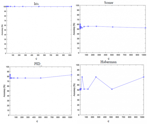
Figure 2. Sensitivity of linear TWSC+ to the hyper-parameter c
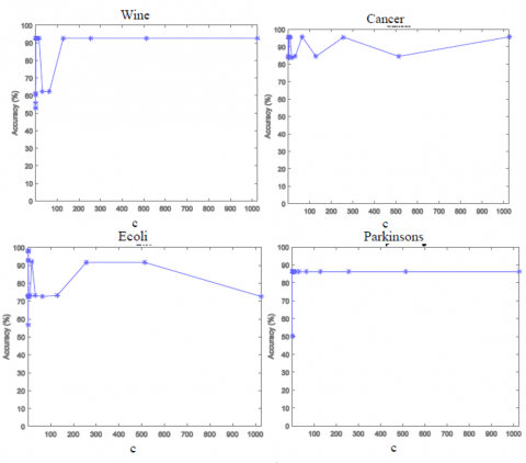
Figure 3. Sensitivity of non-linear TWSC+ to the hyper-parameter c
Figure 2 and Figure 3 depict the sensitivity of linear TWSVC+ and non-linear TWSVC+ to the hyper-parameter c, respectively. As it can be seen, the sensitivity of TWSVC+ to the hyper-parameter c depends on input dataset. For some datasets, when the hyper-parameter c changes the accuracy does not changes; for some datasets, when the hyper-parameter c changes for a wide range the accuracy does not changes; and for some datasets, when the hyper-parameter c changes the accuracy changes.
(1) In this paper, a TWSVM-based clustering model called TWSVC+ was proposed which is an improved version of TWSVC. Our experiments on five real datasets showed that TWSVC+ has the highest accuracy compared with SVC, TWSVC and k-means, and has the less training time compared with SVC and TWSVC.
(2) The accuracy and training time of TWSVC+ is better than SVC because SVC is SVM-based clustering model while TWSVC+ is TWSVM-based clustering model, and training time and accuracy of TWSVM is better than those of SVM [8].
(3) The accuracy and training time of TWSVC+ is better than TWSVC because TWSVC is not a standard model with respect to some of its variables while TWSVC+ is a standard model (QPP) with respect to the mentioned variables. A time-consuming algorithm named concave-convex algorithm is used to solve the non-standard model TWSVC with respect to the mentioned variables while there are efficient algorithms to solve TWSVC+ with respect to the mentioned variables. Moreover, the concave-convex algorithm does not guarantee a global optimal solution with respect to the mentioned variables while QPP does.
|
X |
training set |
|
N |
the number of training data |
|
xi |
i-th training data |
|
Xi |
i-th data cluster |
|
$\widetilde{\mathrm{X}}_{\mathrm{i}}$ |
the other data clusters located on both sides of the i-th cluster center |
|
wi |
weight vector of i-th cluster |
|
bi |
bias of i-th cluster |
|
k |
the number of cluster |
|
thr |
threshold parameter |
|
e, $\tilde{e}$ |
vectors of which elements are equal to 1 |
|
q, $\tilde{q}$ |
slack vectors |
|
Uip |
membership degree of xi to clusters p |
|
w, $\tilde{w}$ |
weight vectors of hyperplanes |
|
b, $\tilde{b}$ |
biases of hyperplanes |
|
$\lambda$ |
a small positive scalar |
|
L |
A threshold parameter |
|
$\alpha, \beta$ |
lagrange coefficients |
|
c, $\tilde{c}$ |
penalty parameter |
[1] Huang, X., Ye, Y., Zhang, H. (2014). Extensions of kmeans-type algorithms: a new clustering framework by integrating intracluster compactness and intercluster separation. IEEE Transactions on Neural Networks and Learning Systems, 25(8): 1433-1446. https://doi.org/10.1109/TNNLS.2013.2293795
[2] Huang, X., Yang, X., Zhao, J., Xiong, L., Ye, Y. (2018). A new weighting k-means type clustering framework with an l2-norm regularization. Knowledge-Based Systems, 151: 165-179. https://doi.org/10.1016/j.knosys.2018.03.028
[3] Yao, M., Wu, Q., Li, J., Huang, T. (2016). K-walks: clustering gene-expression data using a K-means clustering algorithm optimised by random walks. International Journal of Data Mining and Bioinformatics, 16(2): 121-140. https://doi.org/10.1504/IJDMB.2016.080039
[4] Cui, X., Wang, F. (2015). An improved method for K-means clustering. 2015 International Conference on Computational Intelligence and Communication Networks (CICN), Jabalpur, India, pp. 756-759. https://doi.org/10.1109/CICN.2015.154
[5] Suryavanishi, A.S., Gujra, A.D. (2016). A new framework for k-means algorithm by combining the dispersions of clusters. International Journal of Advance Research in Computer Science and Management Studies, 4(1).
[6] Bradley, P.S., Mangasarian, O.L. (2000). K-plane clustering. Journal of Global Optimization, 16(1): 23-32. https://doi.org/10.1023/A:1008324625522
[7] Tabatabaei-Pour, M., Salahshoor, K., Moshiri, B. (2006). A modified k-plane clustering algorithm for identification of hybrid systems. 2006 6th World Congress on Intelligent Control and Automation, Dalian, China. https://doi.org/10.1109/WCICA.2006.1712564
[8] Shao, Y.H., Bai, L., Wang, Z., Hua, X.Y., Deng, N.Y. (2013). Proximal plane clustering via eigenvalues. Procedia Computer Science, 17: 41-47. https://doi.org/10.1016/j.procs.2013.05.007
[9] Liu, L.M., Guo, Y.R., Wang, Z., Yang, Z.M., Shao, Y.H. (2017). K-proximal plane clustering. International Journal of Machine Learning and Cybernetics, 8(5): 1537-1554. https://doi.org/10.1007/s13042-016-0526-y
[10] Zhang, K., Tsang, I.W., Kwok, J.T. (2009). Maximum margin clustering made practical. IEEE Transactions on Neural Networks, 20(4): 583-596. https://doi.org/10.1109/TNN.2008.2010620
[11] Xu, L., Neufeld, J., Larson, B., Schuurmans, D. (2005). Maximum margin clustering. In Advances in Neural Information Processing Systems, pp. 1537-1544.
[12] Wang, Z., Shao, Y.H., Bai, L., Deng, N.Y. (2015). Twin support vector machine for clustering. IEEE transactions on Neural Networks and Learning Systems, 26(10): 2583-2588. https://doi.org/10.1109/TNNLS.2014.2379930
[13] Gunn, S.R. (1998). Support vector machines for classification and regression. ISIS Technical Report, 14(1): 5-16.
[14] Khemchandani, R., Chandra, S. (2007). Twin support vector machines for pattern classification. IEEE Transactions on Pattern Analysis and Machine Intelligence, 29(5): 905-910. https://doi.org/10.1109/TPAMI.2007.1068
[15] Tian, Y., Qi, Z., Ju, X., Shi, Y., Liu, X. (2014). Nonparallel support vector machines for pattern classification. IEEE Transactions on Cybernetics, 44(7): 1067-1079. https://doi.org/10.1109/TCYB.2013.2279167
[16] Chen, S.G., Wu, X.J. (2018). A new fuzzy twin support vector machine for pattern classification. International Journal of Machine Learning and Cybernetics, 9(9): 1553-1564. https://doi.org/10.1007/s13042-017-0664-x
[17] Yuille, A.L., Rangarajan, A. (2002). The concave-convex procedure (CCCP). In Advances in Neural Information Processing Systems, pp. 1033-1040. https://doi.org/10.1162/08997660360581958