Bella Clarisa Meylani![]() | Paiman Eko Prasetyo*
| Paiman Eko Prasetyo*![]()
© 2023 IIETA. This article is published by IIETA and is licensed under the CC BY 4.0 license (http://creativecommons.org/licenses/by/4.0/).
OPEN ACCESS
Volatility in international crude oil prices can have a significant impact on economic stability and potentially disrupt the achievement of sustainable development goals. This research aims to identify the impact of international crude oil prices on Indonesia's monetary sector. The study utilized monthly secondary data from 2017:01-2022:11 and employed a Vector Error Correction Model for analysis. The variables used were International Crude Oil Prices, Inflation, Exchange Rates, and Consumer Expectations Index. The novelty of this research is the inclusion of consumer expectations as a variable. The results show that there is cointegration between the variables, and a reciprocal connection occurs between Exchange Rates and International Crude Oil Prices. The Impulse Response Function analysis indicates that changes in International Crude Oil Prices have a long-term impact on Inflation, Exchange Rates, and Consumer Expectations Index. Based on Forecast Error Variance Decomposition analysis, changes in the International Crude Oil Prices will have a significant impact on Inflation and Exchange Rates. In terms of sustainable development, the increasing crude oil prices may lead to greater consumption of renewable energy through substitution behavior. Mitigation policies can be prepared for both the short and long term phases.
crude oil prices, impact, indonesia, monetary sector, sustainable development
The fossil fuels still have a dominant position for economic sustainability. Crude oil as the main source of fossil fuels has its own role for the realization of sustainable development. The use of fossil fuels has the potential to worsen environmental quality and make climate change even more extreme. This prompted the United Nations to increase the campaign to use renewable energy as the main energy source to become increasingly massive. It is also aligned with the 2030 sustainable development goals on the use of clean (environmentally friendly) and affordable modern energy. Low crude oil prices make the final price of fuel oil cheap and the use of renewable energy will decrease [1].
Beside of final impact on sustainable development, volatility in international crude oil prices as the main source of fuel oil also potentially disrupt macroeconomic performance [2-4] and lead to sustainable challenges, especially for net importing countries [5-7] including Indonesia. The imported crude oil is a crussial thing for Indonesia caused by the insufficient of domestic production to equal the required level of consumption.
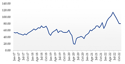
International crude oil prices West Texas Intermediate (WTI) type show an increasing trend from 2017 to the end of 2022 (Figure 1), this is due to a decrease in global crude oil inventories, the Middle East conflict, the agreement on limiting oil production (OPEC-Russia), increased demand crude oil by China, and exacerbated by the geopolitical conflict that occurred between Russia and Ukraine, considering Russia is one of the powerful crude oil producing countries in the world and contributes 11% of global oil production, so that the geopolitical turmoil at there also affected the fluctuations of international crude oil prices. Research findings validate that geopolitical conditions that occur in crude oil exporting countries cause prices volatility on international market [8-10].
Figure 1. International crude oil prices (WTI)
Source: Investing, 2023
The increment in international crude oil prices led to higher the production costs of domestic fuel oil, so this had a significant negative impact on the sustainability of the monetary sector. This happens because the higher cost of fuel production due to the increase in crude oil prices in the international market has the potential to cause inflation from supply side (cost push inflation). As a result of inflation, the stability of the monetary sector will also be disrupted, considering that inflation is an important indicator in the monetary sector that can cause a domino effect for the aggregate economy. At 2022:9, inflation reach 5.95% yoy (highest level in last 5 years), at 2022:11 the rupiah exchange rates ever depreciate into 15,737 IDR/USD, and future economic conditions have the potential to weaken and its lead the consumer expectation to be pesimism. These phenomena are creating a domino effect for the aggregate economy.
The background that have been explained are the base to build the research objectives. So, this research aims to identify the impact of International Crude Oil Prices on the monetary sector which is proxied by the Inflation, Consumer Expectation Index, and Exchange Rates variables. The novelty in this research is a combination of variables involving consumer expectations. This variable is important to analyze because consumers are the parties who receive the final product from processed crude oil, so that fluctuations (especially increment) in oil prices on the international market have the potential to lead changes in the final price received by consumers. Furthermore, economic conditions which are expected continue to deteriorate due to inflation and the depreciation of the rupiah exchange rates will potentially weaken consumer optimism about future conditions, then affecting current consumption patterns. That circumstances makes the impact of crude oil price movements on consumer expectations worthy to analyze. Briefly, this article consists of several main parts, such as introduction, literature review, research methods, results and discussion, and conclusion.
The fuel oil in Indonesia cannot be fully analyzed using a demand – supply approach. Normally, when the price goes up, the demand for that item goes down. However, this is not the case for fuel oil, the value of demand (aggregately) is difficult to reduce even though the price is increasing. Along with the rise in the price level of fuel oil, production costs will also increase [11-13]. If economic conditions do not support for additional capital, companies will be faced with the trilemma, that are increasing the price of output products, reducing the quantity of output products, or reducing other input factors for production cost efficiency. When companies choose to maintain the quantity of output products, the consequence is an increase of production costs (cost push inflation). The research findings was confirmed that the rising of crude oil price drove the increasing on inflation. The contrary research result are not yet found [14-16].
The depreciation of the rupiah exchange rate is inseparable from Indonesia's position as a net importer of crude oil. International trade activities, particularly import, require equivalents value to calculate transaction recapitulation. In the case of crude oil import, the equivalence is carried out using the USD as a benchmark. The higher price of international crude oil, the more Rupiah converted to USD to obtain this commodity, resulting in a weakening of the currency. The research results was validate that the rising of crude oil price led the depreciation of exchange rate in the importing countries [17-19]. But, the findings from another studies [20, 21] are opposite.
Next, the higher of fuel prices will push the production efficiency, such as reducing labor recruitment. Moreover, optimism of consumers to the future conditions in economy are potentially to getting worse as a spillover of higher inflation which is not followed by an increment of income (wages), that condition will transform the consumer behavior. Next, the increment of production costs due to the increase in international crude oil prices are potentially to cause a reduction in employment rate [22, 23]. It will weaken consumer optimism about the availability of jobs in the future. This is based on expectations regarding future conditions, both in terms of income, job availability, and other general economic conditions. This phenomenon is summarized in the Consumer Expectations Index variable, where the measure is generated from calculating the ratio of future consumption compared to current conditions.
This research applies a quantitative method with secondary data on monthly for the 2017:01-2022:11 period sourced from Investing and Central Bank of Indonesia (BI). Quantitative methods are the most appropriate approach to be used in research based on numerical data with clear and measurable objects. This research tries to identify more about the core of the problem that has been arranged systematically by utilizing numerical data that is processed statistically to be able to find answers to the problem formulations that have been compiled. Considering this, quantitative methods are the most appropriate approach to be applied in this research.
The analysis technique applied in this research is Vector Autoregressive (VAR). Compared to other analytical techniques, VAR is the most relevant technique to support the objectives to be achieved in this research. This is because VAR is a time series data analysis technique that is able to estimate the impact of a phenomenon dynamically. In VAR, there are three main models, such as unrestricted VAR, Vector Error Correction Model (VECM), and VAR in difference. The selection of models in VAR is based on the results of the data stationarity test. If stationary data is at the “level”, then the unrestricted VAR model is used, if stationary data is at the “first difference” and cointegration occurs then the VECM model is used, if stationary data at the “first difference” without cointegration then the VAR in difference model is used.
Table 1. Operational definition of variables
|
Variable |
Indicator |
Units |
Source |
|
International Crude Oil Prices (WTI) |
The average of WTI international crude oil prices (monthly). |
USD/barrel |
Investing |
|
Inflation (INF) |
Based on Consumer Price Index (CPI) movements. |
Percent (%) |
BI |
|
Exchange Rates (EXR) |
Monhtly Jakarta Interbank Spot Dollar Rate (JISDOR) IDR/USD in the Foreign Exchange Market. |
IDR/USD |
BI |
|
Consumer Expectations Index (CEI) |
Comparation of consumer expectation on income, general economy condition, and employment rate 6 month later toward present condiotion (ratio) |
Basis point |
BI |
In this technique, all variables act as endogenous variables and estimated simultaneously, so that the relationship between variables can be estimated without identifying exogenous variables. The variables used in this research include (Table 1) International Crude Oil Prices (WTI), Inflation (INF), Exchange Rates, (EXR) and Consumer Expectations Index (CEI).
The Vector Autoregressive (VAR) technique is carried out through several stages which include: (1) Stationarity test, carried out to determine the variance stability of the time series data used. Stationarity testing in this research uses the Augmented Dickey Fuller (ADF) approach. If the test shows a probability of <0.05, then the data is declared stationary at the selected level. If the data is stationary at the “level”, then the unrestricted VAR model can be used. If the data is stationary at the “first difference” and cointegration occurs, then the appropriate model to use is the Vector Error Correction Model (VECM). However, if the data is stationary at the “first difference” without cointegration, then the model used is VAR indifference (2) Selection of the optimum lag, is intended to identify how long the past period of a variable (and other endogenous variables) can affect the condition of the variable at this time. The optimum lag selection in this research is based on the smallest Akaike Information Criteria (AIC) value. (3) Cointegration test, serves to determine the existence of a long-term relationship between variables. In addition, the cointegration test also functions as a model determinant (Vector Error Correction Model or VAR indifference). This test is carried out if the data used is stationary at the first difference. Cointegration in this research was identified using the Johansen approach. Between variables are said to be cointegrated if the value of Trace Statistics or Max Eigen Statistics is greater than the Critical Value value of 0.05. (4) The stability test is a stage that must be fulfilled in a dynamic model such as VAR so that the Impulse Response Function (IRF) and Forecast Error Variance Decomposition (FEVD) analysis are declared valid. The VAR model is declared stable if the modulus value at the Roots of Characteristic Polynomial is less than 1. (5) The estimation of the VAR model is a step that is carried out after the data is declared stable. The basic specification model equation in this research is:
$y_t=\mathrm{c}+\sum_{i=1}^p \emptyset_i y_{t-1}+\varepsilon_t$ (1)
where, $y_t\left(y_{1 t}, y_{2 t}, \ldots y_{n t}\right)$ is the $\mathrm{n} \times 1$ vector of the variables used; $y_{t-i}$ is the variable lag with the order $i$; $ \emptyset_i$ is an $\mathrm{n} \times \mathrm{n}$matrix of autoregressive coefficients and vectors; $y_{t-i}$ for $i=1,2, \ldots, \mathrm{p}, \mathrm{c}=\left(\mathrm{c} 1 . \mathrm{c} 2 \ldots, \mathrm{c}_{\mathrm{n}}\right)$ is $\mathrm{n} \times 1$ intercept vector of the model $\varepsilon_t\left(\varepsilon_{1 t}, \varepsilon_{2 t}, \ldots, \varepsilon_{n t}\right)$ is $\mathrm{n} \times 1$ vector of disturbance (disturbance variable). (6) Causality analysis, is aim to test the existence of a reciprocal connections that occurs among variables. Causality analysis in this research was carried out through the Granger causality test. (7) Impulse Response Function analysis plays a role in identifying the response of endogenous variables to a shock. This response also describes how the impact that occurs from the presence of a shock on the endogenous variables. In this research, Impulse Response Function analysis was carried out to determine the impact that occurred on INF, EXR, and CEI as a result of changes (shocks) that occurred in WTI. (8) Forecast Error Variance Decomposition analysis is a stage for predicting the proportion of variance to changes that occur in the variable itself and other variables.
4.1 Result
The results of this research consist of data stationarity, optimum lag length, cointegration, and model stability testing, followed by the estimation results of the VAR model along with causality analysis, impulse response function analysis, and forecast error variance decomposition. The emphasis on the impact of WTI changes (shocks) on INF, EXR, and CEI is on the Impulse Response Function (IRF) analysis.
1) Stationarity test
Stationarity test results at the “level” show that all variables have a probability >0.05 while at the “first difference” all variables have a probability <0.05 (Table 2). Based on the results, it can be state that the correct model to use is the Vector Error Correction Model (VECM).
Table 2. Result of stationerity test
|
|
Level |
First Difference |
|
WTI |
0.5672 |
0.0000 |
|
INF |
0.3385 |
0.0527 |
|
EXR |
0.1541 |
0.0000 |
|
CEI |
0.1496 |
0.0000 |
2) Testing the optimum lag length
Based on the optimum lag test in Table 3, the smallest AIC value is at lag 1, so that lag 1 is selected as the optimum lag. It means that all subsequent processes, up to the interpretation of using the VAR method, are based on lag 1.
3) Model stability test
The results of the model stability test in Table 4, appear that the modulus value at the Roots of Characteristic Polynomial is less than 1. From these results, declared that the model used is stable or has passed the stability test.
4) Cointegration test
After the stability test, then cointegration testing is carried out. Based on the cointegration test with the Johannsen approach (Table 5), the result is that the trace statistic value is bigger than the critical value of 0.05 on None* and especially on At Most1* or the probability value on the None* row and At most1* row is 0.0016 respectively and 0.0216 (smaller than 0.05).
Table 3. Result of optimum lag tes
|
Lag |
LogL |
LR |
FPE |
AIC |
SC |
HQ |
|
0 |
-1090.741 |
NA |
8.46e+09 |
34.21066 |
34.34559 |
34.26382 |
|
1 |
-889.0061 |
371.9492* |
25551548* |
28.40644* |
29.08109* |
28.67222* |
|
2 |
-876.5475 |
21.41313 |
28720094 |
28.51711 |
29.73148 |
28.99551 |
|
3 |
-864.1896 |
19.69555 |
32681979 |
28.63092 |
30.38502 |
29.32195 |
|
4 |
-850.4277 |
20.21278 |
36091294 |
28.70086 |
30.99468 |
29.60451 |
|
5 |
-845.1149 |
7.139059 |
52911749 |
28.03484 |
31.86837 |
30.15111 |
|
6 |
-831.5642 |
16.51494 |
61538303 |
29.11138 |
32.48463 |
30.44028 |
Table 4. Result of model stability test
|
Root |
Modulus |
|
0.938736 – 0.147275i |
0.950218 |
|
0.938736 + 0.147275i |
0.950218 |
|
0.797624 |
0.797624 |
|
0.435909 – 0.315136i |
0.537892 |
|
0.435909 + 0.315136i |
0.537892 |
|
-0.237428 |
0.237428 |
|
-0.145920 |
0.145920 |
|
0.141172 |
0.14172 |
Table 5. Result of johannsen cointegration test
|
Hypothesized No.Of CE(s) |
Eigenvalue |
Trace Statistic |
0.05 Critical Value |
Prob** |
|
None* |
0.343102 |
61.42528 |
47.85613 |
0.0016 |
|
At most 1* |
0.258089 |
32.84985 |
29.79707 |
0.0216 |
|
At most 2* |
0.126800 |
12.55013 |
15.49471 |
0.1324 |
|
At most 3* |
0.047790 |
3.329957 |
3.841466 |
0.0680 |
From Table 5, it can be stated that the model in this research has cointegration equilibrium equations, or there is a long-term connection among those variables. Thus, it can be confirmed that the Vector Error Correction Model (VECM) model can be used. Next, a VECM model was formed whose results are displayed in Table 6.
5) The result of estimated Vector Error Correction Model (VECM)
The VECM estimation results (Table 6) show that crude oil price at the current period (ΔWTIt) in short-term is positively affected by crude oil prices and the consumer expectations index of the previous period (ΔWTIt-1 and ΔCEIt-1), it variable also negatively affected by inflation and the exchange rates one period earlier (ΔINFt-1 and ΔEXRt-1). The effect of ΔWTIt-1, ΔCEIt-1, and ΔINFt-1 is not statistically significant because the resulting t-statistic value is smaller than the t-table value (1.99547), whereas the ΔEXRt-1 variable has a significant effect. Next, inflation at the current period (ΔINFt) is positively formed by ΔCEIt-1 and ΔEXRt-1, and negatively formed by ΔWTIt-1 and ΔINFt-1. The effect of these four variables is not statistically significant. Furthermore, the current period of consumer expectation index (ΔCEIt) was positively built by ΔWTIt-1 and ΔCEIt-1, and negatively by ΔINFt-1 and ΔEXRt-1.
Table 6. Estimation result of short term VECM
|
|
ΔWTI |
ΔINF |
ΔCEI |
ΔEXR |
|
C0 (S.E) [t-stat] |
0.683421 (0.78447) [0.87118] |
0.036357 (0.03302) [1.10107] |
0.072190 (0.92846) [0.07775] |
36.60113 (46.8160) [0.78181] |
|
ΔWTIt-1 (S.E) [t-stat] |
0.145650 (0.12573) [1.15842] |
-0.003625 (0.00529) [-0.68489] |
0.057816 (0.14881) [-0.38853] |
-0.188234 (7.50342) [-0.02509] |
|
ΔINFt-1 (S.E) [t-stat] |
-4.859157 (2.86369) [-1.69682] |
-0.211592 (0.12054) [-1.75543] |
-3.666114 (3.38932) [1.08167] |
-10.94758 (170.900) [-0.06422] |
|
ΔCEIt-1 (S.E) [t-stat] |
0.152214 (0.10198) [1.49261] |
0.003552 (0.00429) [0.82760] |
0.087271 (0.12070) [0.72306] |
1.734391 (6.08589) [0.28499] |
|
ΔEXRt-1 (S.E) [t-stat] |
-0.006247 (0.00211) [-2.95626]* |
3.06e-05 (8.9E-05) [0.34406] |
-0.006639 (0.00250) [-2.65435]* |
-0.136352 (0.12611) [-1.08117] |
*statistically significant (t-statistic>t-table)
Based on the resulted t-statistic value, only ΔEXRt-1 has a significant effect. Then, the exchange rate at the current period (ΔEXRt) is positively influenced by ΔEXRt-1, and negatively affected by ΔINFt-1, ΔEXRt-1, and ΔWTIt-1. Statistically, the influence of the four variables can be stated to be insignificant.
At the short term, ΔWTIt-1 has negative influence to the ΔINFt and ΔEXRt.. Then, ΔWTIt-1 positif influence on ΔCEIt. Statistically, all the influence of ΔWTIt-1 for another variables are not significant. The coefficient of influence will be more explain through its impacts on other variables by the Impulse Response Function analysis.
VECM estimates (Table 7) show that in the long term INF, EXR, and CEI have a negative effect on WTI. The influence of the three variables is not statistically significant.
Table 7. Estimation result of long term VECM
|
|
WTI |
|
INF (S.E) [t-stat] |
-3.947150 (3.54343) [-1.11393] |
|
CEI (S.E) [t-stat] |
-0.217035 (0.29053) [1.49261] |
|
EXR (S.E) [t-stat] |
-0.010261 (0.00527) [-1.94747] |
6) The result of granger causality test
The granger causality test (Table 8) show the result that EXR and WTI have a causal relationship (two-way), this can be seen from the both probability value <0.05 (significance level 5%).
Table 8. Result of granger causality test
|
Variable |
Toward |
F-statistic |
Prob |
|
INF WTI |
WTI INF |
5.22064 26.7620 |
0.0255 2.E-06 |
|
CEI WTI |
WTI CEI |
0.05342 0.64918 |
0.8179 0.4233 |
|
EXR WTI |
WTI EXR |
5.13944 4.80969 |
0.0266 0.0318 |
|
CEI INF |
INF CEI |
2.73527 2.07214 |
0.1029 0.1547 |
|
EXR INF |
INF EXR |
0.00972 0.47190 |
0.9217 0.4945 |
|
EXR CEI |
CEI EXR |
3.97743 0.33622 |
0.0502 0.5640 |
7) Analysis of Impulse Response Function (IRF)
Based on Figure 2, it can be state that:
At the 1st period to 24th period, INF consistently showed increase response. This can be interpreted that the shocks on WTI has impact to increase of INF. Judging from the graph, INF's response to WTI shocks does not move towards the balance point (0 point). It can be concluded that shocks of WTI have a long term impact on INF.
Next, EXR consistently show a increase response toward shocks on WTI along the 24 periods. This indicates that shocks to WTI have impact weakening of the Exchange Rates (depreciation). The graph shows that EXR's response to WTI shocks does not appear to be moving towards 0 point. It can be concluded that shocks on WTI have long term impact on EXR.
CEI's response to the WTI shock in the first period until second period are downward. This means that in 1st to 2nd period, a shock to WTI have impact in lower of CEI. Furthermore, entering the 3rd to 24th period, CEI continues to show a upward response. This means that shocks on WTI will increase CEI in the 3rd to 24th period. Judging from the resulted IRF graph, the CEI's response to WTI dominantly upward from the 3rd to the 24th period, this indicates that in general WTI shocks have impact on the increase of CEI. The graph shows that the CEI's response to the WTI shock has not moved close to 0 point. It can be concluded that shocks on WTI have long term impact on CEI.
8) Analysis of Forecast Error Variance Decomposition (FEVD)
Based on the FEVD results (Table 9), the findings are:
At the 1st period, the variations in changes on WTI is formed by itself variable (100%). Then in the 12th period, WTI's contribution in explaining changes in itself decreased, in the 36th period it remained at 85.63%. Even though it has consistently experienced a decline, over the next 36 periods the changes in WTI still be dominated by itself.
The variation of changes in INF at the 1st period was dominated by its own contribution (99.83%), then 0.17% was determined by WTI. Interestingly, in the 12th and 36th periods, WTI's contribution rose significantly to 51.39% and 57.88%. Meanwhile, INF's contribution in explaining its own changes continued to decline, remaining 4.38% in the 36th period. Furthermore, EXR also experienced an increase contribution, from 0% in the first period to 37.55% in the 36th period. By that result, it can be state that during the 12th to 36th period, movements of INF are dominantly formed by WTI and EXR contributions.
In the 1st period, the dominant variation of CEI came from self-contribution (95.72%), followed by INF of 4.09%, and WTI of 0.19%. Entering the 12th to 36th period, EXR's contribution continues to increase, even the figure is greater than INF and WTI, but still smaller than CEI. In general, it can be concluded that in the next 36 periods, changes that occur in CEI still be predominantly self-inflicted, followed by EXR, INF, and WTI.
Variations in EXR movements at the 1st period dominantly built by itself (97.23%), then CEI contribute 2.14%, WTI (0.38%), and INF (0.24%). Since the 12th period, WTI's contribution in explaining EXR changes has consistently increased, reaching 55.34% in the 36th period. Next, INF's contribution also consistently increased to 2.94% in the 36th period. CEI's contribution in explaining EXR changes continued to decrease until the 36th period to 1.41%.
Meanwhile, EXR's contribution in explaining changes in itself also gradually decreased until 40.29% at the 36th period. From these results, it can be concluded that in the next 36 periods, changes in EXR will be dominated by WTI and also the variable itself.
Figure 2. The impact of changes in WTI on the monetary sector variables
Table 9. Result of forecast error variance decomposition
|
Variable |
Periods |
S.E |
Variance Decomposition (units in %) |
|||
|
ΔWTI |
ΔINF |
ΔCEI |
ΔEXR |
|||
|
ΔWTI |
1 |
6.3753 |
100.0000 |
0.0000 |
0.0000 |
0.0000 |
|
12 |
22.7594 |
84.7706 |
2.6673 |
5.7282 |
6.8339 |
|
|
24 |
28.7632 |
85.3446 |
2.2846 |
7.2973 |
5.0735 |
|
|
36 |
33.4792 |
85.6332 |
2.0837 |
8.1007 |
4.1825 |
|
|
ΔINF |
1 |
0.2683 |
0.1684 |
99.8316 |
0.0000 |
0.0000 |
|
12 |
1.3465 |
51.3955 |
15.3191 |
0.2025 |
33.0829 |
|
|
24 |
2.3517 |
56.6852 |
6.3568 |
0.2210 |
36.7370 |
|
|
36 |
3.0814 |
57.8440 |
4.3794 |
0.2253 |
37.5511 |
|
|
ΔCEI |
1 |
7.5454 |
0.1942 |
4.0894 |
95.7164 |
0.0000 |
|
12 |
30.6351 |
0.7657 |
2.6697 |
87.0903 |
10.4743 |
|
|
24 |
44.3145 |
1.4574 |
1.8547 |
84.2798 |
12.4080 |
|
|
36 |
54.7453 |
1.7393 |
1.9311 |
83.2026 |
13.1000 |
|
|
ΔEXR |
1 |
380.4637 |
0.3834 |
0.2423 |
2.1424 |
97.2319 |
|
12 |
1021.373 |
31.0164 |
1.3217 |
1.7817 |
65.8803 |
|
|
24 |
1440.969 |
48.5428 |
2.4802 |
1.5197 |
47.4572 |
|
|
36 |
1769.634 |
55.3426 |
2.9547 |
1.4103 |
40.2924 |
|
4.2 Discussion
Significant changes in international crude oil prices lead to increase in inflation [14-16, 24-26]. This condition prompted the government establish a policy to increase the price of fuel oil in the consumer market so that it had an impact on the aggregate economy. Central Bank of Indonesia as the monetary authority has issued a contractionary policy in the form of a discount policy (raising the interest rate) as a response to suppressing the inflation rate. This is not aimed at controlling the rate of inflation from the supply side, but rather the demand side through the money supply. Viewed from the side of the rupiah exchange rates, the increase in international crude oil prices led to depreciation. These findings are in line with empirical studies which show that an increase of international crude oil prices causes a depreciation in the exchange rate in net importing countries as a result of USD demand conversion has increased [5, 17-19, 27].
The reinforcement of USD was pushed by increment interest rates policy by The Fed. The increase in interest rates triggered an increase of capital inflow to the United States [28]. On the other hand, the price of crude oil is set in nominal USD currency, so that when the USD appreciates, the price of oil will also increase [29]. Interestingly, the weakening of the exchange rates after the increase of international crude oil prices did not occur in certain net importer countries such as China, Japan and South Korea [3, 27]. The appreciation of Yuan (China)/USD and Yen (Japan)/USD after increasing international crude oil prices is caused by the devaluation policies and dumping policies set by these countries [30-32], the South Korean Won showed appreciation when the price rose supported by the increasing strength of the Korean Wave when the economy was in expansion phase [33].
The next finding in this research is that the CEI variable shows a decreasing response in the very short term and then consistently increases after passing a turning point in the second period. The decline in CEI in the short term (1-2 periods) occurs due to the potential increase in fuel prices and cause a domino effect in the form of inflation. However, this condition can be overcome because the government immediately responds to shocks to oil prices through various policies, especially intervening in fuel prices by increasing the allocation of subsidy funds. On the other hand, oil price volatility had a major impact on the supply side, thus encourage the monetary authorities to overcome the deteriorating economic conditions from the demand side by maintaining the stability of the business cycle [34].
The ability of the monetary authority to make the business cycle move stably has the potential to maintain the level of employment and people's income, which will eventually result in stability of aggregate demand-supply in the market [34-37]. It shows good general economic conditions, so that CEI is moving up and stable for the long term even though oil prices are experiencing shocks.
Some efforts that can be made to overcome crude oil price shocks in the short term through monetary policy include stabilizing the business cycle through lowering interest rates. This will have an impact on the potential for increasing access to working capital (credit) by producers, so that the effects of cost push inflation can be minimized. Next, the addition of working capital makes production costs still efficient to operate without reducing one of the input factors (labor). Maintained business cycles and employment opportunities have the potential to strengthen consumer optimism regarding the availability of jobs and economic conditions in the future.
Exchange rate stabilization can be carried out through monetary operations in the form of Open Market Operations (OMO) for rupiah and foreign exchange interventions. Several foreign currency OMO instruments that are practical to apply are in the form of spot, forward and Domestic Non Deliverable Fund (DNDF) transaction interventions because they can be executed without going through an auction process. In conditions where the depreciation of the exchange rate continues to occur, the central bank may take Operation Twist (two or more OMO instruments taken simultaneously). The Operation Twist formulation can consist of double rupiah OMO, double foreign currency OMO, as well as rupiah-forex OMO.
In the long term, mitigation of this impact can be supported by upstream and downstream controls. In the upstream sector (oil acquisition), an increase in domestic production must be encouraged. Several actions that can be taken are activation of development wells (new) and maintenance of active (old) wells. This will increase the quantity of oil refineries so that dependence on imported crude oil can be helped. Next, from the diplomatic path, it can be pursued by proposing a bilateral agreement, in which crude oil purchases can be made using local currency units. This can minimize the depreciation of the exchange rate. Next, control of the downstream sector can be pursued by setting proportional fuel prices according to income level categories. Some of the actions that can be taken are increasing the supply of non-subsidized fuel oil, tightening the supply of subsidized fuel oil, and setting certain procedural requirements for production driving fuels, such as diesel. This will have an impact on the burden of controlled fiscal policy.
Beside of upstream and downstream control, in the long run the impact of crude oil price shocks can also be mitigated through structural changes in the economy because it is closely related to the achievement of sustainable development goals. These structural changes can be explained from 2 aspects, namely business behavior and consumption behavior. To change the structure of business behavior, the encouragement towards the realization of sustainable investments must be increased. It can be realized by increasing the ease of access to investment when oil prices are rising. This condition makes the portfolio of environmentally friendly (eco-friendly) companies in the capital market experience positive sentiment and potentially scale up the operational activity with more eco-friendly input factors. The existence of this policy will increase the spillover of energy-friendly business behavior [38, 39].
Next, to control consumption behavior, the government can also realize it through a green fund policy in the form of greater subsidies for environmentally friendly products both in terms of the production process and the inherent nature of the product itself. On the other hand, the increase in oil prices has an impact on increasing renewable energy consumption [40], so that the existence of policies that encourage the use of environmentally friendly products will further strengthen the shift in consumption behavior. The increasingly encouraged shift in consumption from fuel energy to renewable energy makes sustainable development goals faster to be realized.
International crude oil prices have increased significantly in the last five years and led shocks for economic stability and strategy of sustainable development realization, especially for net importing countries such as Indonesia. The results in this empirical study reveal that volatilities in international crude oil prices have an impact on rising inflation, the rupiah exchange rates (depreciation), and the consumer expectations index and this lasts in the long term.
Policies that can be taken as steps to mitigate these impacts can be divided into 2 phases of mitigation. The short-term phase can be realized by controlling interest rates, while the long-term phase can be controlled by countermeasures in the upstream and downstream sectors. In additional, to support the realization of sustainable development goals, the impacts of shocks in crude oil prices can be mitigate by increasing of green investment, green fund, and renewable energy consumption. Limitations in this research are on the subject and the use of variables. The subjects in this research are limited to Indonesia while there are many other net importer countries that may be affected by the increase in international crude oil prices. In addition, the use of variables is limited to three monetary sector indicators only. Further research can take broader research subjects and add other variables related to the monetary sector, so that the discussion can be more complex.
[1] Setyadharma, A., Prasetyo, P.E., Oktavilia, S., Fortuna, B.D., Wahyuningrum, I.F.S. (2022). Does higher income lead to more renewable energy consumption? Evidence from Indonesia. In IOP Conference Series: Earth and Environmental Science, 1098(1): 012081. https://doi.org/10.1088/1755-1315/1098/1/012081
[2] Jiang, Y., Feng, Q., Mo, B., Nie, H. (2020). Visiting the effects of oil price shocks on exchange rates: Quantile-on-quantile and causality-in-quantiles approaches. The North American Journal of Economics and Finance, 52: 101161. https://doi.org/10.1016/j.najef.2020.101161
[3] Hashmi, S.M., Chang, B.H., Huang, L., Uche, E. (2022). Revisiting the relationship between oil prices, exchange rate, and stock prices: An application of quantile ARDL model. Resources Policy, 75: 102543. https://doi.org/10.1016/j.resourpol.2021.102543
[4] Zhang, Y., Hyder, M., Baloch, Z.A., Qian, C., Saydaliev, H.B. (2022). Nexus between oil price volatility and inflation: Mediating nexus from exchange rate. Resources Policy, 79: 102977. https://doi.org/10.1016/j.resourpol.2022.102977
[5] Saidu, M.T., Naseem, N.A.M., Law, S.H., Yasmin, B. (2021). Exploring the asymmetric effect of oil price on exchange rate: Evidence from the top six African net oil importers. Energy Reports, 7: 8238-8257. https://doi.org/10.1016/j.egyr.2021.07.037
[6] Le, T.H., Boubaker, S., Bui, M.T., Park, D. (2023). On the volatility of WTI crude oil prices: A time-varying approach with stochastic volatility. Energy Economics, 117: 106474. https://doi.org/10.1016/j.eneco.2022.106474
[7] Zhao, J. (2022). Exploring the influence of the main factors on the crude oil price volatility: An analysis based on GARCH-MIDAS model with Lasso approach. Resources Policy, 79: 103031. https://doi.org/10.1016/j.resourpol.2022.103031
[8] Kim, M.S. (2018). Impacts of supply and demand factors on declining oil prices. Energy, 155: 1059-1065. https://doi.org/10.1016/j.energy.2018.05.061
[9] Liu, L., Wang, Y., Wu, C., Wu, W. (2016). Disentangling the determinants of real oil prices. Energy Economics, 56: 363-373. https://doi.org/10.1016/j.eneco.2016.04.003
[10] Wang, Q., Sun, X. (2017). Crude oil price: Demand, supply, economic activity, economic policy uncertainty and wars–From the perspective of structural equation modelling (SEM). Energy, 133: 483-490. https://doi.org/10.1016/j.energy.2017.05.147
[11] Husaini, D.H., Lean, H.H. (2021). Asymmetric impact of oil price and exchange rate on disaggregation price inflation. Resources Policy, 73: 102175. https://doi.org/10.1016/j.resourpol.2021.102175
[12] Antonio, J.G., Luis, A.H. (2022). Inflation, oil prices and exchange rates. The Euro’s dampening effect. Journal of Policy Modeling, 44(1): 130-146. https://doi.org/10.1016/j.jpolmod.2021.12.001
[13] Kilian, L., Zhou, X. (2022). The impact of rising oil prices on US inflation and inflation expectations in 2020-23. Energy Economics, 113: 106228. https://doi.org/10.1016/j.eneco.2022.106228
[14] Lacheheb, M., Sirag, A. (2019). Oil price and inflation in Algeria: A nonlinear ARDL approach. The Quarterly Review of Economics and Finance, 73: 217-222. https://doi.org/10.1016/j.qref.2018.12.003
[15] Mien, E. (2022). Impact of oil price and oil production on inflation in the CEMAC. Resources Policy, 79: 103010. https://doi.org/10.1016/j.resourpol.2022.103010
[16] Mukhtarov, S. (2020). The effects of oil prices on macroeconomic variables: Evidence from Azerbaijan. International Journal of Energy Economics and Policy. 10(1): 72-80. https://doi.org/10.32479/ijeep.8446
[17] Sokhanvar, A., Bouri, E. (2023). Commodity price shocks related to the war in Ukraine and exchange rates of commodity exporters and importers. Borsa Istanbul Review, 23(1): 44-54. https://doi.org/10.1016/j.bir.2022.09.001
[18] Zhang, X., Baek, J. (2022). The role of oil price shocks on exchange rates for the selected Asian countries: Asymmetric evidence from nonlinear ARDL and generalized IRFs approaches. Energy Economics, 112: 106178. https://doi.org/10.1016/j.eneco.2022.106178
[19] Wen, D., Liu, L., Ma, C., Wang, Y. (2020). Extreme risk spillovers between crude oil prices and the US exchange rate: Evidence from oil-exporting and oil-importing countries. Energy, 212: 118740. https://doi.org/10.1016/j.energy.2020.118740
[20] Ahmad, W., Prakash, R., Uddin, G.S., Chahal, R.J.K., Rahman, M.L., Dutta, A. (2020). On the intraday dynamics of oil price and exchange rate: What can we learn from China and India? Energy Economics, 91: 104871. https://doi.org/10.1016/j.eneco.2020.104871
[21] Baghestani, H., Toledo, H. (2019). Oil prices and real exchange rates in the NAFTA region. The North American Journal of Economics and Finance, 48: 253-264. https://doi.org/10.1016/j.najef.2019.02.009
[22] Chan, Y.T., Dong, Y. (2022). How does oil price volatility affect unemployment rates? A dynamic stochastic general equilibrium model. Economic Modelling, 114: 105935. https://doi.org/10.1016/j.econmod.2022.105935
[23] Cuestas, J.C., Gil-Alana, L.A. (2018). Oil price shocks and unemployment in Central and Eastern Europe. Economic Systems, 42(1): 164-173. https://doi.org/10.1016/j.ecosys.2017.05.005
[24] Castillo, P., Montoro, C., Tuesta, V. (2020). Inflation, oil price volatility and monetary policy. Journal of Macroeconomics, 66: 103259. https://doi.org/10.1016/j.jmacro.2020.103259
[25] Raheem, I.D., Bello, A.K., Agboola, Y.H. (2020). A new insight into oil price-inflation nexus. Resources Policy, 68: 101804. https://doi.org/10.1016/j.resourpol.2020.101804
[26] Salisu, A.A., Isah, K.O., Oyewole, O.J., Akanni, L.O. (2017). Modelling oil price-inflation nexus: The role of asymmetries. Energy, 125: 97-106. https://doi.org/10.1016/j.energy.2017.02.128
[27] Kisswani, K.M., Elian, M.I. (2021). Analyzing the (a) symmetric impacts of oil price, economic policy uncertainty, and global geopolitical risk on exchange rate. The Journal of Economic Asymmetries, 24: e00204. https://doi.org/10.1016/j.jeca.2021.e00204
[28] Rakhmat, Warjiyo, P., Sadli, A.M. (2022). The influence of exchange rate and foreign capital on the performance of inflation targeting framework in Indonesia. International Journal of Sustainable Development and Planning, 17(5): 1585-1592. https://doi.org/10.18280/ijsdp.170523
[29] Çanakcı, M. (2021). Role of oil prices and major macroeconomic factors in the economic growth of selected G20 countries. International Journal of Sustainable Development and Planning, 16(2): 347-356. https://doi.org/10.18280/ijsdp.160214
[30] Anastasopoulos, A. (2018). Testing for financial contagion: New evidence from the Greek crisis and yuan devaluation. Research in International Business and Finance, 45: 499-511. https://doi.org/10.1016/j.ribaf.2017.09.001
[31] Ludema, R.D., Mayda, A.M., Yu, Z., Yu, M. (2021). The political economy of protection in GVCs: Evidence from Chinese micro data. Journal of International Economics, 131: 103479. https://doi.org/10.1016/j.jinteco.2021.103479
[32] Li, K., Devpura, N., Cheng, S. (2022). How did the oil price affect Japanese yen and other currencies? Fresh insights from the COVID-19 pandemic. Pacific-Basin Finance Journal, 75: 101857. https://doi.org/10.1016/j.pacfin.2022.101857
[33] Baek, J., Nam, S. (2021). The South Korea–China trade and the bilateral real exchange rate: Asymmetric evidence from 33 industries. Economic Analysis and Policy, 71: 463-475. https://doi.org/10.1016/j.eap.2021.06.007
[34] Geiger, M., Scharler, J. (2019). How do consumers assess the macroeconomic effects of oil price fluctuations? Evidence from US survey data. Journal of Macroeconomics, 62: 103134. https://doi.org/10.1016/j.jmacro.2019.103134
[35] Alpanda, S., Granziera, E., Zubairy, S. (2021). State dependence of monetary policy across business, credit and interest rate cycles. European Economic Review, 140: 103936. https://doi.org/10.1016/j.euroecorev.2021.103936
[36] Bui, D.T., Nguyen, C.P., Su, T.D. (2021). Asymmetric impacts of monetary policy and business cycles on bank risk-taking: evidence from Emerging Asian markets. The Journal of Economic Asymmetries, 24: e00221. https://doi.org/10.1016/j.jeca.2021.e00221
[37] Mohimont, J. (2022). Welfare effects of business cycles and monetary policies in a small open emerging economy. Journal of Economic Dynamics and Control, 136: 104316. https://doi.org/10.1016/j.jedc.2022.104316
[38] Wang, Q., Fan, Z. (2023). Green finance and investment behavior of renewable energy enterprises: A case study of China. International Review of Financial Analysis, 87: 102564. https://doi.org/10.1016/j.irfa.2023.102564
[39] Dutta, A., Jana, R.K., Das, D. (2020). Do green investments react to oil price shocks? Implications for sustainable development. Journal of Cleaner Production, 266: 121956. https://doi.org/10.1016/j.jclepro.2020.121956
[40] Guo, Y., Yu, C., Zhang, H., Cheng, H. (2021). Asymmetric between oil prices and renewable energy consumption in the G7 countries. Energy, 226: 120319. https://doi.org/10.1016/j.energy.2021.120319