Yousef Altork*![]() | Malik I. Alamayreh
| Malik I. Alamayreh![]()
© 2024 The authors. This article is published by IIETA and is licensed under the CC BY 4.0 license (http://creativecommons.org/licenses/by/4.0/).
OPEN ACCESS
Optimizing hybrid thermal systems for domestic heating systems is essential to achieve maximum energy efficiency, lower carbon emissions, and decrease overall expenses. This research focuses on utilizing solar energy through evacuated tube solar water systems in conjunction with fuel-based (LPG or diesel) boilers or electric heat pumps for heating residential homes in various climate zones across Jordan. The contributions of each sub-system of thermal energy production were assessed using a one-year dynamic simulation using simulation software TSOL and Meteonorm. A variety of optimization methods are then employed to study and compare several parameters, including station rankings as well as technical and environmental factors. The optimization methods Best-Worst Method BWM yields the highest and lowest weights for the total solar fraction and solar contribution to heating, respectively. After station rankings were conducted using the ARAS, VIKOR, TOPSIS, MOORA, and AHP methodologies, the Maan and Amman stations were identified as most relevant and inappropriate for ETSW use. The annual production of 115.38 GJ utilizing ETSW at the stations under study reduced CO2 emissions by 12.18 tons. The largest losses, accounting for 60.25% and 33.86% of the total losses, respectively, were identified as thermal and optical losses for Maan station. Thus, this study's findings demonstrate the potential of optimized hybrid thermal systems, integrating solar energy with conventional heating methods, to significantly enhance energy efficiency, reduce carbon emissions, and lower overall expenses in residential heating across diverse climate zones in Jordan.
hybrid heating power system, sanitary hot water, carbon dioxide emissions, Best-Worst Method (BWM), economic analysis
Jordan has limited natural resources and high-energy prices. According to the Word Bank organization review, During the last two decades, Jordan's population has also more than doubled to 11 million, increasing the energy demand. Further [1], the Jordanian government estimated that the Jordan population will rise to over 19 million by mid – 2050 [2]. The estimated yearly personal energy consumption rate in Jordan was 1746 kWh on average (as of 2021) [3]. This coupled with climate change is going to have a major impact on energy demand and the amount of usable energy sources available. Action is required immediately to reduce demand, increase supply, and apply the principles of a circular economy to meet future energy requirements.
Jordan is a country that is hugely reliant on imported fossil fuels to meet its energy needs. Referring to the International Renewable Energy Agency (IRENA) Report 2021 [4]. It was illustrated from the report that 4% of the total supply of energy in Jordan came from renewable energy and 96% of the total energy from hydrocarbons fuels (coal, gas, and oil). Furthermore, the report illustrated that only 3% of the energy supply in Jordan increased during the period 2014-2019, while solar energy was the main supply of renewable energy. During 2022, the fossil fuels rapidly increased in Jordan. The Jordanian government raised the prices of oil derivatives many times during the year 2022. The prices of diesel usually used for resident building heating increased by 47% during the period from May 2021 to May 2023. The price of an LPG gas for central disruption increased to 33% according to the Ministry of Energy retail prices of petroleum products [5, 6]. This is due to rises in global energy prices and due to the increase in the energy demand in Jordan.
There are alternative energy sources can be used to reduce the risk of raised prices of oil derivatives including solar thermal energy, heat pumps, and hybrid heating systems. In accord with the report of the Ministry of Energy in Jordan 2021 about 48% of the electrical energy in Jordan quantities in residential buildings [3]. There are many benefits to using hybrid energy systems. They are more efficient than traditional systems, and they can help reduce greenhouse gas emissions, providing sustainable energy and utilizing natural resources optimally. Hybrid systems can also provide backup power in case of a power outage. Due to the oil derivatives price shocks, it is necessary to optimize and select the most adequate domestic heating system depend on the location and weather. It is necessary to find alternative energy sources because fossil fuels contribute to pollution. Hybrid conventional solar collectors are utilized, but their effectiveness is significantly reduced on cold, cloudy, and windy days [7]. In Jordan, some of these hybrid systems are designed with thermal storage systems [8, 9], or without storage systems [10-12].
Researchers have used optimization methods to select the best energy model configurations for a system. Optimizing capacity and operation strategies is crucial to the efficiency of a system. Generally, studies aim to maximize energy efficiency, reduce carbon dioxide emissions, and reduce total annual costs. For example, in Tianjin, China, the researchers Lu et al. [13] developed a bi-level model optimization method suitable for coupled multi-energy systems, which can improve energy efficient and more stably. Comparing the optimized system to the traditional system, 36.2% of annual operating costs can be saved. The researchers Liu et al. [14] used multi-objective optimization technique to optimize distributed energy systems combined with hybrid energy storage and reduce annual global emissions of carbon dioxide by 51.7%–73.2%. The team of Ren et al. [15] discussed using multi-objective optimization technique to improve a hybrid heating and cooling system that integrates solar and geothermal energy sources. According to the results, the hybrid system configuration in China that uses a heat pump with electricity achieves better performance than other configurations. Wu et al. [16] compared configuration and operation optimization methods. Using the collaborative optimization method, multiple decision variables were determined using a genetic algorithm and orthogonal experimental design. Zhang et al. [17] show that it is possible to save 5.5% of energy in a hotel by using multi-population genetic algorithms to enhance a combined cooling, heating and geothermal heat pump. Kalbasi et al. [18] discussed the use of hybridized systems for heating water and spaces in sixteen stations in Belgium. As a result of using TSOL software in energy dynamic simulation, the researchers concluded that evacuated tube solar water with an electric boiler is both cost-effective and attractive. The ARAS technique, VIKOR, and TOPSIS optimization methods were also applied.
The researchers Franco et al. [19] applied a dynamic simulation to study energy systems in a building in Pisa. They concluded that an energy savings of up to 44% could be achieved through occupant-centred control strategies and demand-controlled ventilation in large non-residential buildings. Multi-objective optimization approach applied by the researchers [20] Based on different scenarios relating to climate change and energy price aberration, the method is applied to a building in Tehran. As a result of energy retrofitting, up to 73% of CO2 emissions can be reduced, and thermal discomfort can be reduced by up to 46%. For buildings’ space heating loads in the integrated community energy system, the researcher Jin et al [21] conducted a numerical study to demonstrate that a balanced scheduling scheme can be obtained with a bi-level model predictive control method by balancing consumer energy costs with the profits of the operator of an integrated community energy system (ICES). The model predictive control (MPC) was based mixed-integer linear program that formulated as an optimization of a bilevel model predictive control model using the Karush-Kuhn-Tucker optimality conditions. The researchers [22] formulate and develop computationally efficient heuristics for solving the optimal power-water-heat flow problem. By combining convex relaxation and convex–concave procedures, the proposed heuristic is able to solve the OPWHF in an iterative manner. The simulation shows that the proposed framework improves the operational flexibility of the integrated system during periods of time-varying energy prices and photovoltaic generation. In order to optimize HVAC systems in buildings, Lu et al. [23] employed adaptive neuro-fuzzy inference systems. The simulation study compares the optimization method with traditional methods. Based on the results, the proposed method significantly increases system performance.
The objective of this research is to determine the overall heating capacity required for a residential building across six locations in Jordan, employing three variations of a central hybrid heating system. These systems incorporate an evacuated tube solar collector in conjunction with either an auxiliary boiler or a heat pump. The research can illustrate which central heating system is more suitable depending on the location and climate in Jordan.
Figure 1 illustrates the Global Horizontal Irradiation (GHI) in Jordan, a Middle Eastern country covering an expanse of 89,213 square kilometers, with around 75% of its landmass classified as desert terrain [24].
In Jordan, the climate is predominately Mediterranean; there are too short transitional periods in the year: the first begins around the beginning of October, and the second about the middle of April. The climate in Aqaba and the Dead Sea is characterized by a hot and dry desert climate compared to Amman, which has a Mediterranean climate that is milder [25]. Figure 1 shows long term (1999-2018) average global horizontal irradiation AGHR in Jordan and selected cities for different regions in Jordan. The range AGHR in Jordan is between 2000-2900 kWh/m2, while Maan has the highest global radiation more than 2900 kWh/m2. In this research, six selected cities for different regions in Jordan were obtained, namely. Amman, Aqaba, Maan, Karak (Ghor El Safi), Irwaished, and Irbid to cover most climates in Jordan.
Figure 1. Global horizontal irradiation in Jordan and selected cities for different regions in Jordan [26]
The objective of this study is to optimize and compare three central heating system types: (1) a hybrid central heating system consists of a solar collector and gas boiler. (2) A hybrid central heating system consists of a solar collector with diesel boiler. (3) A hybrid central heating system consist of a solar collector and heat pump. This research also evaluates and compares various optimization methods, which include:
• Additive Ratio Assessment (ARAS)
• TOPSIS method
• VIKOR method
• Multi-Objective Optimization based on Ratio Analysis (MOORA)
• Analytic Hierarchy Process (AHP)
Furthermore, the research will discuss the impact of factors such as CO2 emissions avoided, heating solar fraction, system efficiency, economic effect, and the impact of climate data in six locations in Jordan. Then, the research tries to optimize the best configurations. The novelty of this research lies in its ability to demonstrate the optimal hybrid heating system tailored to the unique combination of location in Jordan and climate data.
2.1 TSOL software
The current research involves one-year simulations that were conducted at six different stations in Jordan. Since conducting experiments for this many stations in just one year are not feasible, it is recommended to use reliable software like TSOL for simulations within this scope. The accuracy of TSOL's results has been demonstrated in previous studies cited in articles [27-29].
TSOL is a software tool specifically designed for simulating solar thermal systems, including various components like water heat storage units, pools, and heating processes. The software calculates the required energy balance and heating capacity based on hourly typical weather data [28]. TSOL considers both the beam radiation and diffuse radiation, where the diffuse intensity is determined through a formula when the collector is tilted at an angle of α, as the beam radiation is available in climate libraries.
$\begin{gathered}0 \leq k_t \leq 0.3: \frac{I_d}{I}=1.02-0.245 k_t+0.0123 \sin \alpha \\ 0.3<k_t \leq 0.78: \frac{I_d}{I}=1.4-1.749 k_t+0.177 \sin \alpha \\ k_t>0.78: \frac{I_d}{I}=0.486 k_t-0.182 \sin \alpha\end{gathered}$ (1)
where, $k_t$ indicates the hourly allowance index, $I$, which represents the total hourly irradiance on a horizontal surface $\left[\frac{\mathrm{kJ}}{\mathrm{m}^2}\right]$, and $I_d$, represents the surface's hourly diffuse irradiance $\left[\frac{\mathrm{kJ}}{\mathrm{m}^2}\right]$. The formula for calculating collector thermal energy dissipation [29] is given by:
$\begin{aligned} \rho=G_{\text {dir }} \cdot \eta_0 \cdot f_{I A M} & +G_{ {diff }} \cdot \eta_0 \cdot f_{ {IAM.diff }} -k_0\left(T_{k m}-T_A\right)-k_q\left(T_{k m}-T_A\right)^2\end{aligned}$ (2)
The equation includes several variables, such as $\eta_0$, which represents the collector's zero-loss efficiency, $G_{d i r}$, which is the portion of solar irradiation that strikes a tilted surface, $f_{ {IAM }}$, which is the modifier for the incident angle, $G_{ {diff }}$, which is the diffuse solar irradiance that strikes a tilted surface, $f_{ {IAM.diff }}$, which is the modifier for the diffuse incident angle, $k_0$, which is the heat transfer coefficient (measured in $\frac{W}{m^2 \cdot k}$, $T_{k m}$, which is the collector average temperature, $T_A$, which is the ambient temperature, and $k_q$, which is the heat transfer coefficient (measured in $\frac{W}{m^2 \cdot k^2}$ ).
The losses in solar collectors due to optics determined by running an energy balance between the collectors' input irradiance and output energy, using parameters such as the "incident angle modifier" and "conversion factor" that are specific to the type of collector. To estimate the reduction in pollutants resulting from using SWHs, the TSOL software calculates the primary energy saved and based on fuel type-specific emission parameters to determine the heating system's carbon dioxide emissions. For natural gas fuel, TSOL software employs an emitted at a rate of 5.144 g CO2/kJ [29].
The energy provided by the solar thermal system is divided by the total heat given to the standby tank (from both solar and auxiliary boiling sources), as shown below, to determine the overall solar fraction, which reflects the percentage of standby tank energy supplied by solar energy.
$Solar\, fraction _{ {Total }}=\frac{Q_{C L . D H W}+Q_{ {S.HL }}}{Q_{ {CL.DHW }}+Q_{ {S.HL }}+Q_{ {AuxH.DHW }}+Q_{ {AuxH.HL }}}$ (3)
Other relations related to the current simulation, according to Figure 2 are illustrated as following [29]:
$Solar\, fraction_{D H W}=\frac{Q_{C L . D H W}}{Q_{C L . D H W}+Q_{A u x H . D H W}}$ (4)
$Solar\, fraction_{ {Heating }}=\frac{Q_{S . H L}}{Q_{S . H L}+Q_{A u x H . H L}}$ (5)
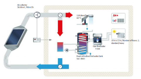
The research proposes to employ two distinct systems: a solar air heater and a solar water heater, both of which are coupled to an extra 9 kW boiler as shown in Figure 2. The proposed system depicted in Figure 2(a), which is widely used in different countries such as Algeria, Canada, and Turkey in previous studies [27-29], has been selected for the current research. As a consequence, the suggested system has been used in this investigation since, as the findings section will show, it is more extensively used and more efficient than the method in Figure 2(b).
Figure 2. (a) The solar water heating system's diagram with auxiliary 9 kW boiler (gas fired, oil-fired, or heat pump). (b) The solar air heating system's diagram with auxiliary 9 kW boiler
2.2 Best-Worst Method (BWM)
The optimal choice is chosen using the MCDM method for making decisions across multiple criteria, which compares multiple options based on several indexes. The best and worse choices are made by the decision-maker based on Rezaei's best-worst technique [30], and then pairs each of these two indicators with other indicators to compare them to one another. The weights of the different indexes are then determined by formulating and solving a MAXIMIN problem. A correlation is also considered in this method to assess the incompatibility rate and ensure that the comparison is valid. The following steps make up the BWM approach [30]:
$\begin{array}{r}{minmax}_j\left\{\left|\frac{w_B}{w_j}-s_{B j}\right|,\left|\frac{w_j}{w_w}-s_{j w}\right|\right\} \text { s.t. } \sum_j w_j =1, \quad w_j \geq 0, { for \,all } \,j\end{array}$ (6)
By simplifying Eq. (6) yields:
$\begin{gathered}min \,\xi \text { s.t. }\left|\frac{w_B}{w_j}-s_{B j}\right| \leq \xi, { for \, all }\, j \\ min\, \xi \text { s.t. }\left|\frac{w_j}{w_w}-s_{j w}\right| \leq \xi, { for \,all }\, j \\ \sum_j w_j=1, w_j \geq 0, { for \,all }\, j\end{gathered}$ (7)
The liner model of Eq. (7) can be expressed as [31]:
$\begin{gathered}min\, \xi \text { s.t. }\left|w_B-s_{B j} w_j\right| \leq \xi, { for\, all\, } j \\ min\, \xi \text { s.t. }\left|w_j-s_{j w} w_w\right| \leq \xi, { for \,all\, } j \\ \sum_j w_j=1, w_j \geq 0, { for \,all\, } j\end{gathered}$ (8)
The optimum values of $\left\{w_1^*, w_2^*, \cdots, w_n^*\right\}$ are determined by solving Eq. (8). The compatibility rate is calculated using $\xi^*$. A greater value of $\xi^*$ obviously signifies a higher compatibility rate. The highest value of $\xi$ can be found since $a_{B j} * a_{j w}=a_{B W}$ and $a_{B W} \in\{1,2, \ldots, 9\}$.
The degree of compatibility indicators listed in Table 1 and Eq. (9) are used to compute the consistency ratio [30]:
$Consistency \,Ratio =\frac{\xi^*}{ { Consistency \,index }}$ (9)
The consistency ratio becomes closer to zero as the outcomes become more reliable.
Table 1. consistency index using BWM
|
sBW |
Consistency Index (max $\xi$) |
|
1 |
0.00 |
|
2 |
0.44 |
|
3 |
1.00 |
|
4 |
1.63 |
|
5 |
2.3 |
|
6 |
3.00 |
|
7 |
3.73 |
|
8 |
4.47 |
|
9 |
5.23 |
The level of idealization is utilized in the ARAS approach to order the alternatives [32, 33]. Three stages make up the ARAS method [32]. The m×n decision-matrix is designed in the first step, where m is the number of choices (rows), and n is the number of criteria (columns).
$R=\left[\begin{array}{ccccc}r_{01} & \cdots & r_{0 j} & \cdots & r_{0 n} \\ \vdots & \ddots & \vdots & \ddots & \vdots \\ r_{i 1} & \cdots & r_{i j} & \cdots & r_{i n} \\ \vdots & \ddots & \vdots & \ddots & \vdots \\ r_{m 1} & \cdots & r_{m j} & \cdots & r_{m n}\end{array}\right] i=\overline{0, m} ; j=\overline{1, n}$ (10)
The function of the i-th option in the j-th criterion is represented by $r_{i j}$. The optimum value for the j criterion is also $r_{0 j}$. The optimum value of the j variable is established by Eq. (11).
$\begin{aligned} & r_{i j}=\max _i r_{i j}, \text { if } \max _i r_{i j} \text { is preferable } ; \\ & r_{i j}=\min _i r_{i j}, \text { if } \min _i r_{i j} \text { is preferable. }\end{aligned}$ (11)
The initial decision matrix's values are converted to values that fall between (0-1) and (0-∞) using the normalizing technique. The second stage involves normalizing the initial input values for each criterion to the form $\bar{r}_{i j}$, which corresponds to the elements of the matrix $\bar{R}$ and is defined by Eq. (12).
$\bar{R}=\left[\begin{array}{ccccc}\bar{r}_{01} & \cdots & \bar{r}_{0 j} & \cdots & \bar{r}_{0 n} \\ \vdots & \ddots & \vdots & \ddots & \vdots \\ \bar{r}_{i 1} & \cdots & \bar{r}_{i j} & \cdots & \bar{r}_{i n} \\ \vdots & \ddots & \vdots & \ddots & \vdots \\ \bar{r}_{m 1} & \cdots & \bar{r}_{m j} & \cdots & \bar{r}_{m n}\end{array}\right] i=\overline{0, m} ; j=\overline{1, n}$ (12)
The following criteria, whose maxima represent the preferred values, are normalized:
$\bar{r}_{i j}=\frac{r_{i j}}{\sum_{i=0}^m r_{i j}}$ (13)
By using a two-stage process, the criteria, whose preferred values are minima, are normalized:
$r_{i j}=\frac{1}{r_{i j}^*}, \bar{r}_{i j}=\frac{r_{i j}}{\sum_{i=0}^m r_{i j}}$ (14)
In the third step, the normalized matrix $\bar{R}$ is combined with the weights to create the matrix $\hat{R}$. $w_j$ stands for the weight of each $\mathrm{j}$-criterion.
$\hat{R}=\left[\begin{array}{ccccc}\hat{r}_{01} & \cdots & \hat{r}_{0 j} & \cdots & \hat{r}_{0 n} \\ \vdots & \ddots & \vdots & \ddots & \vdots \\ \hat{r}_{i 1} & \cdots & \hat{r}_{i j} & \cdots & \hat{r}_{i n} \\ \vdots & \ddots & \vdots & \ddots & \vdots \\ \hat{r}_{m 1} & \cdots & \hat{r}_{m j} & \cdots & \hat{r}_{m n}\end{array}\right] i=\overline{0, m} ; j=\overline{1, n}$ (15)
$\hat{r}_{i j}=\bar{r}_{i j} * w_j$ (16)
The optimality function values are specified by the following equation:
$S_i=\sum_{j=1}^n \hat{r}_{i j}, i=\overline{0, m}$ (17)
where, $S_i$ represents the value of the option i's optimality function. Each option's alternative utility is determined by contrasting it with the best value, designated $S_0$. According to Eq. (18) the utility degree equation $\left(K_i\right)$, is found for option $A_i$. Consider the fact that $K_i$ values are used to rank the alternatives.
$K_i=\frac{S_i}{S_0}, i=\overline{0, m}$ (18)
This method takes into account both the choice's distance from the epitome point and its distance from the undesirable ideal one. The preferred option needs to be the furthest from the ideal point while also being the furthest from the opposite ideal point [34]. Both benefit and cost measures can be calculated using TOPSIS [35]. The vector normalization approach is utilized in the TOPSIS method to normalize the criteria. Using Eq. (19) [36], the normal value of $r_{i j}$ is calculated:
$r_{i j}=\frac{x_{i j}}{\sum_{i=1}^M x_{i j}^2}$ (19)
where, $r_{i j}$ is the value of the typical decision matrix and $x_{i j}$ is the value for the option i according to criterion j. The formula for the typical balanced beta decision matrix is calculated by applying Eq. (20) to the normal decision matrix V and a set of weights W = (w1, w2,…, wn):
$v_{i j}=w_{i j} * r_{i j}$ (20)
Following that, using Eqs. (21) and (22) as a basis, the ideal solutions ($A^*$) and ($A^{-}$) are calculated:
$\begin{gathered}A^*=\left\{\left(\max v_{i j} \mid j \in J\right),\left(\min v_{i j} \mid j \in J^{\prime}\right) \mid i=1,2,3, \ldots, M\right\} =\left\{v_{1^*}, v_{2^*}, \ldots, v_{N^*}\right\}\end{gathered}$ (21)
$\begin{gathered}A^{-}=\left\{\left(\min v_{i j} \mid j \in J\right),\left(\max v_{i j} \mid j \in J^{\prime}\right) \mid i=1,2,3, \ldots, M\right\} =\left\{v_{1^{-}}, v_{2^{-}}, \ldots, v_{N^{-}}\right\}\end{gathered}$ (22)
The Euclidean technique and Eqs. (23) and (24) are used to determine how far option j is from the optimum situation ($s_i^*$) and the worst-case situation ($s_i^{-}$):
$s_i^*=\sqrt{\sum_{j=1}^n\left(v_{j i}-v_j^*\right)^2}, i=1, \cdots, M$ (23)
$s_i^{-}=\sqrt{\sum_{j=1}^n\left(v_{j i}-v_j^{-}\right)^2}, i=1, \cdots, M$ (242)
Then, using Eq. (25), it is calculated how close each choice ($A_j$) is to the ideal answer:
$C_{i^*}=\frac{S_{i^{-}}}{S_{i^*}+S_{i^{-}}}, 0 \leq C_{i^*} \leq 1, i=1,2,3, \ldots, M$ (25)
Finally, the options are ranked in order of importance using $C_{i^*}$'s value.
Inconsistent and disproportionate criterion decision problems were the motivation for the development of VIKOR. The VIKOR model bases ranking on how close a solution is to the ideal one. Four steps make up the VIKOR technique [37, 38].
Step 1: Using Eq. (26), the optimum ideal solution $f_j^*$ (PIS) and the undesirable ideal solution $f_j^{-}$ (NIS) are derived:
$\begin{aligned} & f_j^*=\left\{\max _i f_{i j} \mid j \in I_1\right\}, f_j^*=\left\{\min _i f_{i j} \mid j \in I_2\right\} \\ & f_j^{-}=\left\{\min _i f_{i j} \mid j \in I_1\right\}, f_j^{-}=\left\{\max _i f_{i j} \mid j \in I_2\right\}\end{aligned}$ (26)
where, I1 and I2 are, correspondingly, a set of profit and cost criteria.
Step 2: $S_i$ and $R_i$ values are determined using the Eqs. (27) and (28):
$S_i=\sum_{j=1}^n w_j\left(f_j^*-f_{i j}\right) /\left(f_j^*-f_j^{-}\right)$ (27)
$R_i=\max _j\left[w_j\left(f_j^*-f_{i j}\right) /\left(f_j^*-f_j^{-}\right)\right]$ (28)
where, $w_j$ is the weighted criteria.
Step 3: Using Eq. (29) to calculate the $Q_i$ index:
$Q_i=v\left(\frac{S_i-S^*}{S^{-}-S^*}\right)+(1-v)\left(\frac{R_i-R^*}{R^{-}-R^*}\right)$ (29)
where, $S^*=\min S_i, S^{-}=\max S_i, R^*=\min R_i, R^{-}=$ $\max R_i$, and the weights $v$ and $(1-v)$ represent attractiveness and regret, respectively. Depending on the decision-maker, $v$ can have any value between 0 and 1.
Step 4: The higher the priority and rank, the lower the $Q_i$ value.
MOORA is a technique for multi-objective optimization with discrete options is proposed by WK Brauers and Zavadskas [39]. The approach begins with a matrix of alternate responses to various objectives:
$X=\left[\begin{array}{ccccc}x_{01} & \cdots & x_{0 j} & \cdots & x_{0 n} \\ \vdots & \ddots & \vdots & \ddots & \vdots \\ x_{i 1} & \cdots & x_{i j} & \cdots & x_{i n} \\ \vdots & \ddots & \vdots & \ddots & \vdots \\ x_{m 1} & \cdots & x_{m j} & \cdots & x_{m n}\end{array}\right] i=\overline{0, m} ; j=\overline{1, n}$ (30)
where, alternative j's response to objective i is represented by $x_{i j}$. i = 1, 2, . . . , m are the objectives, j = 1, 2, . . .,n are the alternatives.
An alternative's reaction to an objective is compared to a denominator that is typical of all choices pertinent to that aim using a ratio system called MOORA. The square root of the whole of the squares for each choice per objective is selected as the denominator as follow:
$r_{i j}=\frac{x_{i j}}{\sqrt{\sum_{i=1}^M x_{i j}^2}}$ (31)
where, $r_{i j}$ is a dimensionless number that represents alternative j's normalized response to objective i. These normalized alternatives' responses to objectives are within the range [0:1].
The formula for the typical balanced beta decision matrix is calculated by applying Eq. (32) to the normal decision matrix and a set of weights $w_{i j}$ = (w1, w2,…, wn):
$v_{i j}=w_{i j} * r_{i j}$ (32)
These responses are added for maximum and subtracted for minimization in the optimization process:
$Y_i=\sum_{i=1}^g v_{i j}-\sum_{i=g+1}^n v_{i j}$ (33)
with i = 1, 2, . . . , g for the purposes to be maximized, i = g + 1, g + 2, . . . , n for the purposes to be minimized. $Y_i$ is the normalized evaluation of option j in relation to all objectives. Linearity in this expression refers to dimensionless measurements in the range between 0 and 1. The final preference is shown by an ordinal ranking of the $Y_i$.
When making decisions to address complicated issues, the Analytic Hierarchy Process (AHP) is applied with multiple criteria or alternatives. Developed by Saaty [40], AHP broadly used in various fields, for instance: engineering, economics, social sciences, and environmental studies.
The basic idea behind AHP is to break down a complex decision problem into smaller, more manageable parts, and after that compare each component's relative importance using pairs of evaluations. By doing so, AHP offers a well-structured framework for making decisions, and helps decision-makers to clarify their preferences and priorities. The AHP method divided into the following steps:
Step 1: Structure the issue: Create a decision hierarchy, define the decision problem, and list the criteria and alternatives.
Step 2: Pairwise comparison: Evaluate the relative importance of each criterion and alternative by pairwise comparisons using a 9-point scale. The scale ranges from 1 (equally important) to 9 (extremely more important). Assuming, for instance, that criterion A is twice as significant as criterion B, then A given a value of 2 and B a value of 1/2.
Step 3: Weight calculation: Calculate the weights of the criteria and alternatives by normalizing the comparison matrix for pairs. The weights are the relative importance of each criterion and alternative, and they should add up to one. To calculate the weight of criterion i, the ith column's sum divided by the comparison pairs matrix. The pairwise comparison matrix is divided by the sum of the jth row in order to determine the weight of alternative j.
Step 4: Consistency check: By calculating the consistency index (CI) and consistency ratio (CR), you may determine whether the pairwise comparison matrix is consistent. The CI is a measure of how consistent the judgments are, and the CR is a ratio of the CI to a random consistency index. If the CR is less than 0.1, the judgments considered consistent.
Step 5: Aggregation: Aggregate the weights of the criteria and alternatives to get an overall ranking. The aggregation done in several ways, such as multiplying the weights of the criteria and alternatives or using a weighted sum.
Here is the equation for normalizing the pairwise comparison matrix:
$W_{i j}=\frac{A_{i j}}{\sum_j A_{i j}}$ (34)
where, $W_{i j}$ is the weight of criterion i relative to criterion $\mathrm{j}, A_{i j}$ is the judgment of criterion i compared to criterion $j$, and $\sum_j A_{i j}$ is the sum of the ith column.
Here is the equation for computing the consistency index:
$C I=\frac{\lambda_{\max }-n}{n-1}$ (35)
where, $\lambda_{\max }$ is the pairwise comparison matrix's highest eigenvalue, and n is the number of criteria or options.
Here is the equation for computing the consistency ratio:
$C R=\frac{C I}{R I}$ (36)
where, RI is the random consistency index, which depends on the size of the pairwise comparison matrix as shown in Table 2.
Table 2. Consistency of random matrices for AHP method
|
Matrix Order |
RI |
|
1 |
0 |
|
2 |
0 |
|
3 |
0.52 |
|
4 |
0.89 |
|
5 |
1.11 |
|
6 |
1.25 |
Data on temperature, location, the temperature of the water distribution network, and the total yearly radiation are shown in Table 3 for specific sites. It should be mentioned that the information in Table 3 was compiled using the Meteonorm 8.0.3 program.
The simulation's results used an assumption that the average household would use 110 liters of hot water per day at a temperature of 60 °C. The simulation was done for the entire year, considering an 80 m2 conditioned space with a temperature of 21°C and a heat load of 10 kW. The double-glazed windows have areas of 1.60, 4.00, 8.00, and 5.60 m2 for the north, east, south, and west, respectively. The heating source's heat gain was estimated to be 5 [W/m2], and the need for space heating was uniform throughout the cold months during the year, from November to April. The building walls were of medium thickness. The solar water heating (SWH) system and accessories, such as buffer tanks, piping length, and boilers, were taken into consideration to enable a fair comparison between various stations. The simulated system used a 20 m2 evacuated tube collector oriented to zero azimuth angle. Dual-coil (300 liters) and single-coil (1000 liters) buffer tanks were used for sanitary hot water and space heating, respectively. The nominal capacity of the gas, diesel, and heat pump boilers was 9 kW, and the volume flow rate of the intermediate fluid, a 60:40 mixture of water and polypropylene glycol, was 40 [liters/m2.h]. For circumstances, the return temperature difference was calculated to be 20 °C when there was a strong demand for space heating and 15 °C in other circumstances. Figure 2 displays a schematic of the simulated system. The solar collector's tilt was set to 45°.
The simulation conducted in this study involves four main steps, each comprising several internal steps and data. These steps include determining user data, obtaining climate data from the Meteonorm software, analyzing the data using the TSOL program, and finally, identifying the optimal location. The first step, determining user data, entails specifying the building requirements for heating purposes, such as the desired amount and temperature of hot water, as well as the solar system specifications. In the second step, climate data is gathered from the Meteonorm software, including location data, total solar radiation, and the percentage of diffuse solar radiation. Both the first and second steps serve as inputs for the third step, which involves analyzing the data using the TSOL program. This analysis focuses on various parameters, such as the total solar fraction, solar contribution to heating, heating solar fraction, DHW solar fraction, solar contribution to DHW, CO2 emissions reduction, fuel savings, and system efficiency. Finally, the last step involves assessing six locations in Jordan to determine the most suitable location for installing the solar system. This assessment considers the assigned weights for each criterion from step three. Various approaches, including ARAS, VIKOR, TOPSIS, MOORA, and AHP, are applied in this evaluation process.
Table 3. Station required data
|
Station |
Latitude |
Longitude |
Total Annual Irradiance [GJ/m2] |
Diffuse Irradiance Percentage [%] |
Cold Water Temperature (Feb/Aug) [˚C] |
|
Maan Airp. |
30.17 ° |
-35.78 ° |
8.028 |
36.7 |
15.5/21 |
|
GHOR EL SAFI (Karak) |
31.03 ° |
-35.46 ° |
7.508 |
36.0 |
23/28.5 |
|
Irwaished |
32.5 ° |
-38.2 ° |
7.684 |
34.9 |
17/23 |
|
Amman Airp. |
31.98 ° |
-35.98 ° |
7.480 |
37.9 |
15.5/20.2 |
|
AQABA INTL AIRPORT |
29.63 ° |
-35.01 ° |
7.867 |
33.6 |
22.5/28 |
|
Irbid |
32.55 ° |
-35.85 ° |
7.329 |
38.2 |
15.5/20 |
Table 4 illustrates the output data corresponding to each system as depicted in Figure 2. Upon examination of the outcomes for the Amman station, it is evident that the solar water heating system exhibits superior performance across all evaluated indices, encompassing system efficiency, avoided CO2 emissions, solar fraction, and fuel saving.
Table 4 presents the results of one-year dynamic simulations. The results indicate that the Aqaba and Amman stations had the highest and lowest performance, respectively, with the former supplying 99.55% and the latter supplying 75.81% of the total required heating demand through Evacuated Tube Solar Water (ETSW). The average total solar fraction for the stations studied in Jordan was found to be 87.49%, based on the results. The stations in Maan, Irwaished, Amman, and Irbid had a total solar fraction lower than the average (i.e., less than 87.49%), indicating that they may not be as appropriate for the intended purpose.
In terms of the thermal power needed for space heating, Maan station has the highest solar contribution with 8.388 GJ per year, while Ghor El-Safi station has the lowest with 2.843 GJ per year. The total solar power transferred for heating annually is 34.898 GJ, which results in an average heating power of 5.816 GJ per station. This average heating power produced by each station is equivalent to a heating solar fraction of 75.94%.
Regarding the potential for providing sanitary hot water, Maan and Ghor El-Safi stations have the highest and lowest solar contribution amounts, respectively. The installation of ETSW in Maan resulted in a supply of 10.202 GJ/year of hot water, while for Ghor El-Safi station, this figure was 9.023 GJ/year. In total, the solar contribution to domestic hot water (DHW) for all the stations under study was 58.485 GJ, resulting in an average supply of hot water power of 9.748 GJ per station. This average supply of hot water power is equivalent to a DHW solar fraction of 99.61%.
Regarding the avoidance of CO2 emissions resulting from the non-utilization of fossil fuels, Maan station is considered the most efficient with an annual CO2 emission avoidance of 1923.10 kg, 1,478.50 kg, and 1,375.70 kg when using diesel, gas, and heat pump auxiliary boilers, respectively. On the other hand, Ghor El-Safi station is the least efficient with an annual CO2 emission avoidance of 1,384.80 kg, 1,064.60 kg, and 878.10 kg for the same auxiliary boilers. The average annual CO2 emission avoidance for each station using the same auxiliary boilers are 1675.85 kg, 1288.40 kg, and 1151.71 kg. In total, all stations combined will avoid emitting 8.23 tons of CO2 emissions per year.
9.1 Weighting of indices
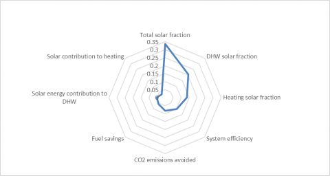
Figure 3 displays the outcomes of the BWM method's final weighting of the indexes based on meeting with several academic researchers in the field of renewable energy as clarified by Kalbasi et al. [18]. It is evident from the results that "Total solar fraction" and "DHW solar fraction" carry the most significant weight, while "Solar contribution to heating" has the least weight. A comparison of the index weights can be observed in Figure 3. Additionally, the BWM technique's consistency ratio for the indexes is 0.07306381.
Figure 3. Comparison of the weight of indexes
9.2 Ranking of stations
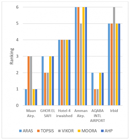
Figure 4 displays the outcomes of a study that assessed the suitability of different stations using five optimization techniques: ARAS, TOPSIS, VIKOR, MOORA, and AHP. The techniques used a method ranking index, such as Ki, Yi, and Qi, to rank the stations. The study revealed that Maan station was the most suitable according to three out of five optimization techniques, while Aqaba station was ranked first in two methods. The ranking presented in Figure 4 was based on a diesel auxiliary boiler. However, when a gas-powered auxiliary boiler was used, the same ranking was obtained as shown in Table 5. In contrast, when a heat pump was used as an auxiliary boiler, the order of some intermediate stations changed, although the first and last preferred stations remained the same.
Table 4. The outputs for each station
|
Location |
System Efficiency |
Total Solar Fraction |
DHW Solar Fraction |
Solar Energy Contribution to DHW [GJ] |
Heating Solar Fraction |
Solar Contribution to Heating [GJ] |
Fuel Savings |
CO2 Emissions Avoided [kg] |
||||
|
Oil-Fired Boiler [L] |
Gas-Fired Boiler [m3] |
Heat Pump [kWh Electricity] |
Oil-Fired Boiler |
Gas-Fired Boiler |
Heat Pump |
|||||||
|
The solar water heating system's diagram with auxiliary 9 kW boiler as in Figure 2(a) |
||||||||||||
|
Maan Airport. |
0.1101 |
0.8731 |
0.9986 |
10.202 |
0.7574 |
8.388 |
722.8 |
699.2 |
2,065.70 |
1,923.10 |
1,478.50 |
1,375.70 |
|
Karak (Ghor el safi) |
0.0757 |
0.9933 |
0.9988 |
9.023 |
0.9763 |
2.843 |
520.4 |
503.5 |
1,318.40 |
1,384.80 |
1,064.60 |
878.1 |
|
Irwaished |
0.1043 |
0.8533 |
0.9965 |
9.935 |
0.7141 |
7.328 |
678.6 |
656.5 |
1,918.10 |
1,805.50 |
1,388.20 |
1,277.40 |
|
Amman Airport. |
0.105 |
0.7581 |
0.9934 |
10.101 |
0.5519 |
6.401 |
657.1 |
635.7 |
1,833.50 |
1,748.50 |
1,344.20 |
1,221.10 |
|
Aqaba airport |
0.0789 |
0.9955 |
1 |
9.122 |
0.9852 |
3.887 |
554.1 |
536 |
1,445.50 |
1,474.30 |
1,133.40 |
962.7 |
|
Irbid |
0.1048 |
0.7763 |
0.989 |
10.102 |
0.5712 |
6.051 |
646 |
624.9 |
1,794.80 |
1,718.90 |
1,321.50 |
1,195.30 |
|
The solar air heating system's diagram with auxiliary 9 kW boiler as in Figure 2(b) |
||||||||||||
|
Amman Airport. |
0.065 |
0.7330 |
0.9420 |
9.347 |
0.5212 |
5.205 |
579.2 |
510.7 |
1427.90 |
1,468.40 |
1,165.10 |
1,005.80 |
Table 5. The outputs of ARAS, TOPSIS, VIKOR, MOORA, and AHP techniques
|
ARAS |
TOPSIS |
VIKOR |
MOORA |
AHP |
|||||||
|
Location |
Type |
Ki |
Rank |
TOPSIS score |
Rank |
Qj |
Rank |
Yi |
Rank |
Yi |
Rank |
|
Maan Airp. |
Oil-fired boiler |
0.145288888 |
1 |
0.563640027 |
3 |
0.165442786 |
3 |
0.424713996 |
1 |
0.926854382 |
1 |
|
GHOR EL SAFI |
Oil-fired boiler |
0.141639488 |
3 |
0.677652911 |
2 |
0.106699213 |
2 |
0.412766177 |
3 |
0.901313906 |
3 |
|
Hotel-4 irwaished |
Oil-fired boiler |
0.140046855 |
4 |
0.468840561 |
4 |
0.381581446 |
4 |
0.409234588 |
4 |
0.894741424 |
4 |
|
Amman Airp. |
Oil-fired boiler |
0.129812393 |
6 |
0.259087471 |
6 |
0.934670484 |
5 |
0.379440412 |
6 |
0.83359929 |
6 |
|
AQABA INTL AIRPORT |
Oil-fired boiler |
0.144243661 |
2 |
0.712718768 |
1 |
0.010070757 |
1 |
0.420507377 |
2 |
0.917176491 |
2 |
|
Irbid |
Oil-fired boiler |
0.130540722 |
5 |
0.266286238 |
5 |
0.947052684 |
6 |
0.381520915 |
5 |
0.837960855 |
5 |
|
Location |
Type |
||||||||||
|
Maan Airp. |
Gas-fired boiler |
0.145286491 |
1 |
0.563627025 |
3 |
0.165442786 |
3 |
0.424704272 |
1 |
0.926854382 |
1 |
|
GHOR EL SAFI |
Gas-fired boiler |
0.141638608 |
3 |
0.677676562 |
2 |
0.106697187 |
2 |
0.41276175 |
3 |
0.901318833 |
3 |
|
Hotel-4 irwaished |
Gas-fired boiler |
0.14006035 |
4 |
0.469062236 |
4 |
0.381216078 |
4 |
0.409273338 |
4 |
0.894845288 |
4 |
|
Amman Airp. |
Gas-fired boiler |
0.129810269 |
6 |
0.259060844 |
6 |
0.934662893 |
5 |
0.37943163 |
6 |
0.833600242 |
6 |
|
AQABA INTL AIRPORT |
Gas-fired boiler |
0.144241317 |
2 |
0.712728469 |
1 |
0.01010154 |
1 |
0.420498548 |
2 |
0.917172611 |
2 |
|
Irbid |
Gas-fired boiler |
0.130538279 |
5 |
0.266257426 |
5 |
0.947052684 |
6 |
0.381511199 |
5 |
0.837959732 |
5 |
|
Location |
Type |
||||||||||
|
Maan Airp. |
Heat pump |
0.146028798 |
1 |
0.578517441 |
3 |
0.165442786 |
3 |
0.427024913 |
1 |
0.926854382 |
1 |
|
GHOR EL SAFI |
Heat pump |
0.140300932 |
4 |
0.651500521 |
2 |
0.107149745 |
2 |
0.408899756 |
4 |
0.889842559 |
4 |
|
Hotel-4 irwaished |
Heat pump |
0.140519758 |
3 |
0.484268234 |
4 |
0.378872283 |
4 |
0.410750158 |
3 |
0.893389053 |
3 |
|
Amman Airp. |
Heat pump |
0.129991687 |
6 |
0.279253315 |
6 |
0.934808663 |
5 |
0.38008311 |
6 |
0.830575358 |
6 |
|
AQABA INTL AIRPORT |
Heat pump |
0.14328139 |
2 |
0.690146875 |
1 |
0.009558775 |
1 |
0.417758844 |
2 |
0.907800244 |
2 |
|
Irbid |
Heat pump |
0.130631517 |
5 |
0.284794018 |
5 |
0.947052684 |
6 |
0.381900123 |
5 |
0.834464357 |
5 |
Figure 4. A comparison of each station's ranking using ARAS, TOPSIS, VIKOR, MOORA, and AHP
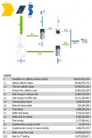
9.3 Assessing the amount of loses in Maan station
Eq. (4) from the "Help" section of the TSOL software provides more information on the heat losses for solar water heaters. First the energy received by the collectors can be calculated and then calculate the optical losses by deducting the energy output and heat losses. Depending on the length of the pipe, both convective and conductive heat transfer are responsible for the heat loss in the pipes.
From Figure 5, it can see that the solar collector receives 168.825 GJ of radiation, and each of the 20 solar collectors receives 8.44 GJ/m2. The radiation on the horizontal surface in Maan is 8.028 GJ/m2, as shown in Table 3. The tilted surface is what causes the difference in energy that the collector receives. The SWH at Maan station experiences 49.282 GJ of optical losses. As the temperature of the solar collector’s increases, heat loss amplifies, and it becomes 87.7 GJ. Figure 5 shows that losses in tanks constitute only 3.5% of the total losses (145.547 GJ). Overall, the loss analysis for this station shows that heat losses, then optical losses, are the main causes of losses. The least amount of losses occur in the buffer tank, main tank, internal piping, and external piping.
Figure 5. Energy balance illustration for Maan station
9.4 Economics analysis of using ETSW
This section focuses on the economics of using ETSW to provide a portion of the building's heating needs as well as sanitary hot water usage. Payback time [41-43] is used to evaluate economic analysis and can be computed using the formula below:
$\begin{aligned} & { Payback \,Time [years] } =\frac{{ Total \,cost \,to \,purchase \,and\, install\, SWH \,system }}{ { Cost \,savings\, per\, year \,owing \,to \,using\, SWH }}\end{aligned}$ (37)
ETSW with HWST initially costs $13000 to purchase and install. On the other hand, the power needed for pumping can be computed simply using the power consumption of 0.025 kWh/m2 [44]. The ability to save energy for each station is shown in Figure 6, which demonstrates that the energy-saving ranges from 5311.9 kWh/year (for Ghor El Safi) to 7376.6 kWh/year (for Maan).
Figure 6. Energy saving potential in each station due to SWH system
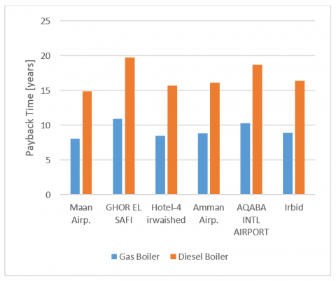
In two distinct examples, the payback time's economic calculations were examined. In the first case, space heating and sanitary hot water were both provided by a hybrid system that included a gas boiler and ETSW. Figure 7 displays the payback time results based on a 0.85% gas boiler efficiency and a $0.06 per kWh natural gas pricing according to the average natural gas price in Jordan in 2022. The cost of using the SWH system is recouped economically in the best and least fortunate stations, respectively, in 8.1 (for Maan) and 10.9 (for Ghor El Safi) years.
Figure 7. Payback time evaluation for each station for a hybrid gas or diesel boiler with ETSW
In the second case, the thermal energy needed to meet the building's heating needs was provided by a diesel boiler hybrid system with ETSW. The payback time results are displayed in Figure 7 and assume a 90% efficiency for the diesel boiler and a fuel cost of $0.18 per kWh according to the average diesel price in Jordan in 2022.
Like the first case, calculations revealed that the payback times for Maan (best) and Gore El Safi (worst) are 14.9 and 19.7 years, respectively. When the first and second cases are compared, it becomes clear that using a gas boiler makes expenditures in the usage of ETSW to meet the building's heating needs more appealing.
The payback period for the hybrid heat pump and ETSW system is long, equaling more than 50 years in Maan station, due to the high cost of the heat pump system and Jordan's relatively affordable electricity pricing. This enormous gap between costs and savings indicates how difficult it will be for the nation to implement sustainable energy alternatives. The long payback period for the hybrid heat pump and ETSW system can deter people and businesses from making the necessary up-front investments, even though they promise improved energy efficiency and diminished environmental impact in the long run.
Various communities have adopted solar energy as a source of hot water delivery because of rising energy costs, a lack of fossil fuels, and environmental concerns. This study uses a central heating system that comprises evacuated tube solar collectors and a backup boiler; diesel, gas, or heat pump to assess the overall heating capacity of a residential structure at six locations throughout Jordan. Software programs TSOL 5.5 and Meteonorm 8.0.3 were used to run simulations. The ARAS, VIKOR, TOPSIS, MOORA, and AHP approaches were used to assess each location's performance.
Key findings of the study include:
In conclusion, this analysis underscores the potential of evacuated tube solar collectors in significantly reducing CO2 emissions, meeting substantial domestic heating demand, and delineating optimal installation locations in Jordan. Future research avenues may focus on further optimizing hybrid heating systems and addressing thermal and optical loss factors to enhance overall efficiency and sustainability.
|
AGHR |
Average Global horizontal irradiation, kWh/m2 |
|
AHP |
Analytic Hierarchy Process |
|
ARAS |
Additive Ratio Assessment method |
|
ARENA |
International Renewable Energy Agency |
|
BWM |
Best-Worst Method |
|
DHW |
Domestic Hot Water |
|
ETSW |
Evacuated Tube Solar Water |
|
LPG |
Liquefied Petroleum Gas |
|
MCDM |
Multi-Criteria Decision Making |
|
MOORA |
Multi-Objective Optimization based on Ratio Analysis |
|
SWH |
Solar Water Heating |
|
TOPSIS |
Technique for Order of Preference by Similarity to Ideal Solution |
|
$\eta_0$ |
The collector's zero-loss efficiency |
|
$G_{ {diff }}$ |
The diffuse solar irradiation that strikes a tilted surface, kWh/m2 |
|
$G_{ {dir }}$ |
The portion of solar irradiation that strikes a tilted surface, kWh/m2 |
|
$I$ |
Total hourly radiation on a horizontal surface, kWh/m2 |
|
$I_d$ |
Hourly diffuse radiation on a horizontal surface, kWh/m2 |
|
$T_A$ |
Ambient temperature, k |
|
$T_{k m}$ |
Collector mean temperature, k |
|
$f_{I A M}$ |
The modifier for the incident angle |
|
$f_{ {IAM.diff }}$ |
The modifier for the diffuse incident angle |
|
$k_0$ |
Heat transfer coefficient, W/m2.k |
|
$k_q$ |
Heat transfer coefficient, W/m2.k2 |
|
$k_t$ |
Hourly clearance index |
[1] World Bank Organization. Jordan Overview. https://www.worldbank.org/en/country/jordan/overview, accessed on Sep. 16, 2023.
[2] Department of Statistics, Jordan Government. Report: Population Projections for the Kingdom’s Residents during the Period 2015-2050. (2016). http://www.dos.gov.jo/dos_home_e/main/Demograghy/2017/POP_PROJECTIONS(2015-2050).pdf, accessed on Sep. 16, 2023.
[3] Minister of Energy & Mineral Resources. Annual Report (2021). https://www.memr.gov.jo/ebv4.0/root_storage/en/eb_list_page/annual_report_2021_en.pdf, accessed on Sep. 16, 2023.
[4] International Renewable Energy Agency (IRENA). Renewables Readiness Assessment: The Hashemite Kingdom of Jordan. https://www.irena.org/publications/2021/Feb/Renewables-Readiness-Assessment-The-Hashemite-Kingdom-of-Jordan, accessed on Sep. 16, 2023.
[5] Minister of Energy & Mineral Resources. (2023). https://www.memr.gov.jo/EBV4.0/Root_Storage/AR/EB_List_Page/p1-5-2023.pdf, accessed on Sep. 16, 2023.
[6] Minister of Energy & Mineral Resources. (2022). https://www.memr.gov.jo/ebv4.0/root_storage/en/eb_list_page/pfy2020-1.pdf, accessed on Sep. 16, 2023.
[7] Hamdan, M., Al Louzi, R., Al Aboushi, A., Abdelhafez, E. (2022). Enhancement of solar water disinfection using Nano catalysts. Journal of Ecological Engineering, 23(12): 14-20. https://doi.org/10.12911/22998993/154775
[8] Al Afif, R., Ayed, Y., Maaitah, O.N. (2023). Feasibility and optimal sizing analysis of hybrid renewable energy systems: A case study of Al-Karak, Jordan. Renewable Energy, 204: 229-249. https://doi.org/10.1016/j.renene.2022.12.109
[9] Alamayreh, M.I., Alahmer, A. (2023). Design a solar harvester system capturing light and thermal energy coupled with a novel direct thermal energy storage and nanoparticles. International Journal of Thermofluids, 18: 100328. https://doi.org/10.1016/j.ijft.2023.100328
[10] Al-Amayreh, M.I., Alahmer, A., Manasrah, A. (2020). A novel parabolic solar dish design for a hybrid solar lighting-thermal applications. Energy Reports, 6(9): 1136-1143. https://doi.org/10.1016/j.egyr.2020.11.063
[11] Srinivas, T., Reddy, B.V. (2014). Hybrid solar–biomass power plant without energy storage. Case Studies in Thermal Engineering, 2: 75-81. https://doi.org/10.1016/j.csite.2013.12.004
[12] Asfar, J.A., Alrbai, M., Qudah, N. (2023). Energy analysis of a hybrid parabolic trough collector with a steam power plant in Jordan. Energy Exploration & Exploitation, 41(6). https://doi.org/10.1177/01445987231188152
[13] Lu, S., Li, Y., Xia, H. (2018). Study on the configuration and operation optimization of CCHP coupling multiple energy system. Energy Conversion and Management, 177: 773-791. https://doi.org/10.1016/j.enconman.2018.10.006
[14] Liu, Z., Fan, G., Sun, D., Wu, D., Guo, J., Zhang, S., Yang, X., Lin, X., Ai, L. (2022). A novel distributed energy system combining hybrid energy storage and a multi-objective optimization method for nearly zero-energy communities and buildings. Energy, 239: 122577. https://doi.org/10.1016/j.energy.2021.122577
[15] Ren, F., Wang, J., Zhu, S., Chen, Y. (2019). Multi-objective optimization of combined cooling, heating and power system integrated with solar and geothermal energies. Energy Conversion and Management, 197: 111866. https://doi.org/10.1016/j.enconman.2019.111866
[16] Wu, D., Han, Z., Liu, Z., Li, P., Ma, F., Zhang, H., Yin, Y., Yang, X. (2021). Comparative study of optimization method and optimal operation strategy for multi-scenario integrated energy system. Energy, 217: 119311. https://doi.org/10.1016/j.energy.2020.119311
[17] Zhang, Y., Deng, Y., Zheng, Z., Yao, Y., Liu, Y. (2023). Optimizing the operation strategy of a combined cooling, heating and power system based on energy storage technology. Scientific Reports, 13(1): 2928. https://doi.org/10.1038/s41598-023-29938-6
[18] Kalbasi, R., Jahangiri, M., Mosavi, A., Dehshiri, S.J.H., Dehshiri, S.S.H., Ebrahimi, S., Etezadi, Z.A.S., Karimipour, A. (2021). Finding the best station in Belgium to use residential-scale solar heating, one-year dynamic simulation with considering all system losses: economic analysis of using ETSW. Sustainable Energy Technologies and Assessments, 45: 101097. https://doi.org/10.1016/j.seta.2021.101097
[19] Franco, A., Miserocchi, L., Testi, D. (2021). A method for optimal operation of HVAC with heat pumps for reducing the energy demand of large-scale non-residential buildings. Journal of Building Engineering, 43: 103175. https://doi.org/10.1016/j.jobe.2021.103175
[20] Mostafazadeh, F., Eirdmousa, S.J., Tavakolan, M. (2023). Energy, economic and comfort optimization of building retrofits considering climate change: A simulation-based NSGA-III approach. Energy and Buildings, 280: 112721. https://doi.org/10.1016/j.enbuild.2022.112721
[21] Jin, X., Wu, Q., Jia, H., Hatziargyriou, N. (2021). Optimal integration of building heating loads in integrated heating/electricity community energy systems: A Bi-level MPC approach. IEEE Transactions on Sustainable Energy, 12(3): 1741-1754. https://doi.org/10.1109/TSTE.2021.3064325
[22] Fang, S., Wang, C., Lin, Y., Zhao, C. (2021). Optimal energy scheduling and sensitivity analysis for integrated power–water–heat systems. IEEE Systems Journal, 16(4): 5176-5187. https://doi.org/10.1109/JSYST.2021.3127934
[23] Lu, L., Cai, W., Xie, L., Li, S., Soh, Y. (2005). HVAC system optimization-in-building section. Energy and Buildings, 37(1): 11-22. https://doi.org/10.1016/J.ENBUILD.2003.12.007
[24] El-Harami, J. (2014). The diversity of ecology and nature reserves as an ecotourism attraction in Jordan. In SHS Web of Conferences, 12: 01056. https://doi.org/10.1051/shsconf/20141201056
[25] Abdulla, F. (2020). 21st century climate change projections of precipitation and temperature in Jordan. Procedia Manufacturing, 44: 197-204. https://doi.org/10.1016/j.promfg.2020.02.222
[26] SolarGIS. Solar Resource Maps of Jordan. https://solargis.com/maps-and-gis-data/download/Jordan, accessed on Sep. 16, 2023.
[27] Siampour, L., Vahdatpour, S., Jahangiri, M., Mostafaeipour, A., Goli, A., Shamsabadi, A.A., Atabani, A. Techno-enviro assessment and ranking of Turkey for use of home-scale solar water heaters. Sustainable Energy Technologies and Assessments, 43: 100948. https://doi.org/10.1016/j.seta.2020.100948
[28] Jahangiri, M., Alidadi Shamsabadi, A., Saghaei, H. (2018). Comprehensive evaluation of using solar water heater on a household scale in Canada. Journal of Renewable Energy and Environment, 5(1): 35-42. https://doi.org/10.30501/jree.2018.88491
[29] Pahlavan, S., Jahangiri, M., Alidadi Shamsabadi, A., Khechekhouche, A. (2018). Feasibility study of solar water heaters in Algeria, a review. Journal of Solar Energy Research, 3(2): 135-146.
[30] Rezaei, J. (2015). Best-worst multi-criteria decision-making method. Omega, 53: 49-57. https://doi.org/10.1016/j.omega.2014.11.009
[31] Rezaei, J. (2016). Best-worst multi-criteria decision-making method: Some properties and a linear model. Omega, 64: 126-130. https://doi.org/10.1016/j.omega.2015.12.001
[32] Zavadskas, E.K., Turskis, Z. (2010). A new additive ratio assessment (ARAS) method in multicriteria decision-making. Technological and Economic Development of Economy, 16(2): 159-172. https://doi.org/10.3846/tede.2010.10
[33] Mostafaeipour, A., Dehshiri, S.J.H., Dehshiri, S.S.H. (2020). Ranking locations for producing hydrogen using geothermal energy in Afghanistan. International Journal of Hydrogen Energy, 45(32): 15924-15940. https://doi.org/10.1016/j.ijhydene.2020.04.079
[34] Hwang, C.L., Yoon, K. (1981). Methods for multiple attribute decision making. Multiple Attribute Decision Making, Springer, Berlin, Heidelberg, 58-191. https://doi.org/10.1007/978-3-642-48318-9_3
[35] Jahangiri, M., Shamsabadi, A.A., Mostafaeipour, A., Rezaei, M., Yousefi, Y., Pomares, L.M. (2020). Using fuzzy MCDM technique to find the best location in Qatar for exploiting wind and solar energy to generate hydrogen and electricity. International Journal of Hydrogen Energy, 45(27): 13862-13875. https://doi.org/10.1016/j.ijhydene.2020.03.101
[36] Triantaphyllou, E. (2000). Multi-criteria decision-making methods. Multi-Criteria Decision-Making Methods: A Comparative Study, Boston, MA: Springer, 5-21. https://doi.org/10.1007/978-1-4757-3157-6_2
[37] Wang, Y.L., Tzeng, G.H. (2012). Brand marketing for creating brand value based on a MCDM model combining DEMATEL with ANP and VIKOR methods. Expert Syst Appl, 39(5): 5600-5615. https://doi.org/10.1016/j.eswa.2011.11.057
[38] Chaghooshi, A., Arab, A., Dehshiri, S. (2016). A fuzzy hybrid approach for project manager selection. Decision Science Letters, 5(3): 447-460. https://doi.org/10.5267/j.dsl.2016.1.001
[39] Brauers, W.K., Zavadskas, E.K. (2006). The MOORA method and its application to privatization in a transition economy. Control and Cybernetics, 35(2): 445-469.
[40] Saaty, T.L. (1986). Axiomatic foundation of the analytic hierarchy process. Management Science, 32(7): 841-855. https://doi.org/10.1287/mnsc.32.7.841
[41] Huang, D., Yu, T. (2017). Study on energy payback time of building integrated photovoltaic system. Procedia Engineering, 205: 1087-1092. https://doi.org/10.1016/j.proeng.2017.10.174
[42] Kong, M., Hong, T., Ji, C., Kang, H., Lee, M. (2020). Development of building driven-energy payback time for energy transition of building with renewable energy systems. Applied Energy, 271: 115162. https://doi.org/10.1016/j.apenergy.2020.115162
[43] Liu, W., Kalbasi, R., Afrand, M. (2020). Solutions for enhancement of energy and exergy efficiencies in air handling units. Journal of Cleaner Production, 257: 120565. https://doi.org/10.1016/j.jclepro.2020.120565
[44] García, J.L., Porras-Prieto, C.J., Benavente, R.M., Gómez-Villarino, M.T., Mazarrón, F.R. (2019). Profitability of a solar water heating system with evacuated tube collector in the meat industry. Renewable Energy, 131: 966-976. https://doi.org/10.1016/j.renene.2018.07.113