Mohammad Sanjeed Hasan* | Rabindra Nath Mondal | Giulio Lorenzini
© 2019 IIETA. This article is published by IIETA and is licensed under the CC BY 4.0 license (http://creativecommons.org/licenses/by/4.0/).
OPEN ACCESS
The present paper investigates numerical simulation of fluid flow and heat transfer through a rotating curved square channel of curvature ratios ranging from 0.001 to 0.5. Crank-Nicolson and Adams-Bashforth methods together with the function expansion and the collocation methods are applied to obtain the numerical solution. The bottom wall of the channel is heated while cooling from the ceiling. The channel is rotated in the positive direction for the Taylor number $0 \leq \operatorname{Tr} \leq 2000$ and combined effects of the centrifugal, Coriolis and buoyancy forces are investigated. As a result, two branches of asymmetric steady solutions comprising with two- to multi-vortex solutions are obtained. Linear stability analysis shows that the flow is stable only for a small region $164.82 \leq T r \leq 601.62$ while unstable otherwise. In the unstable region, time-dependent solutions are obtained and flow transitions are well determined by obtaining power spectrum density of the solutions and it is found that the time-dependent flow undergoes through various flow instabilities, if Tr is increased in the positive direction. The results clearly show the existence of multiple Dean vortices along the duct while axial velocity profile is related to the outer Dean vortices, the wall pressure is more influenced by the Dean vortices attached to the outer concave wall. The present study elucidates the role of secondary vortices on convective heat transfer which shows that convective heat transfer is significantly enhanced by the secondary flow; and the chaotic flow, which takes place at large Tr’s, enhances heat transfer more efficiently than the steady-state or periodic solutions. This study also reveals that there is a sharp influence between the ardor-induced buoyancy force and centrifugal-Coriolis instability in the rotating curved channel that inspires fluids mixing and consequently enhances heat transfer in the fluid. Finally, our numerical results are compared with the experimental investigations, and it is found that there is a good agreement between the numerical and experimental data.
rotating curved channel, dean number, Taylor number, Grashof number, secondary flow, time evolution, heat transfer, chaos
Fluid flow through curved ducts and channels has been extensively studied over a wide range of applications with a key base of heat transfer and mixing enhancement. Such motivation has provided a fairly comprehensive knowledge of physics and numerical modeling addressing intrinsic vortex-structure promoting mixing and momentum transfer. Today, the flows in curved non-circular ducts are of increasing importance in micro-fluidics, where lithographic methods typically produce channels of square or rectangular cross-section. These channels are extensively used in many engineering applications, such as in turbo-machinery, refrigeration, air conditioning systems, heat exchangers, rocket engine, internal combustion engines and in modern gas turbines. In a curved channel, it is strongly anticipated that centrifugal forces are originated in the flow due to curvature causing an opposite directional rotating vortex motion acted on the axial flow through the duct that generates the properties of spiraling fluid flow in the curved passage known as secondary flow. At a convinced precise flow condition and beyond, an additional pair of counter-rotating vortices develops at the outer concave wall of the curved channel which is widely known as Dean vortices [1]. After that, many theoretical and experimental studies have been conducted by considering this flow in mind, here the articles by Berger et al. [2], Nandakumar and Masliyah [3], Zhang et al. [4], Yanase et al. [5] and Mondal et al. [6] may be referenced.
Considering the non-linear nature of the Navier-Stokes equation, the existence of multiple solutions does not come as a surprise. The solution structure of fully developed flow is commonly present in a bifurcation diagram which consists of a number of lines or branches connecting different possible solutions. These branches can bifurcate and show multiple solutions in limit points. Cheng et al. [7] and Shantini and Nandakumar [8] studied flow characteristics in a curved square channel while Finlay and Nandakumar [9], Thangam and Hur [10] and Yanase et al. [5] for a rectangular curved channel. Selmi et al. [11] and Dennis and Ng [12] both analyzed the effects of rotation and flexure on the bifurcation feature of two-dimensional (2D) fluid flow through a rotating curved square-shaped duct. However, a complete bifurcation study of 2D flow through a curved square duct was conducted by Winters [13]. He determined that the isolated symmetric 4-cell sub-branch is unstable while the isolated 2-cell sub-branch is stable. The location of limit point and bifurcation points does not change much for curvature ratios less than 0.02, but at higher curvature ratios, they move to large Dn numbers. Yanase et al. [5] carried out a comprehensive bifurcation study of laminar flow through a curved rectangular duct over a wide range of aspect ratio. They obtained many steady solutions and established a principle that may select realizable one among them. Mondal et al. [6] performed spectral numerical study on fully developed bifurcation structure and stability of 2D flow through a curved square duct and found a close relationship between the unsteady solutions and the bifurcation diagram of steady solutions. Four types of steady solution structures for non-isothermal flows have been also traced out by Hasan et al. [14].
Chandratilleke [15] formulated an improved simulation model based on three-dimensional (3D) vortex structures for describing secondary flow and its thermal characteristics. Wu et al. [16] performed numerical study of the secondary flow characteristics in a curved square duct by using the spectral method, where three walls of the duct, except the outer wall, rotate around the centre of curvature and an azimuthal pressure gradient was imposed. In that study, multiple solutions with two-, four-, eight-vortex and even non-symmetric vortices were obtained at the same flow condition. Very recently, Li et al. [17] studied Dean instability and secondary flow in 120° curved rectangular ducts with continuously varying curvature. In that study, a new criterion based on vortex-core velocities was proposed to more accurately detect the onset of multiple Dean vortices.
Unsteady solution of fully developed curved channel flows was first studied by Yanase and Nishiyama [18]. In that study, they investigated unsteady solutions for the case where dual solutions exist. Unsteady behavior of the flow in a curved rectangular channel of large aspect ratio was investigated, in detail, by Yanase et al. [5] numerically. They performed time-evolution calculations of the flow with and without symmetry condition and showed that periodic oscillations appear with symmetry condition while aperiodic time variation without symmetry condition. Wang and Yang [19] conducted numerical as well as empirical exploration of periodic oscillations for the fully developed flow in a curved square duct. Flow visualization in the range of Dean numbers from 50 to 500 was conducted in their experiment. They showed, both experimentally and numerically, that a temporal oscillation takes place between symmetric/asymmetric 2-cell and 4-cell flows when there are no stable steady solutions. Mondal et al. [20] also have tried to show the flow variation in the unsteady solutions through curved square duct for both positive and negative rotation. They have also narrated the heat transfer effects due to the positive rotation. The nature of secondary flow in a curved square duct was performed by using flow visualization method by Yamamoto et al. [21] experimentally. Liu and Wang [22] performed bifurcation and stability of fully-developed forced convection in a tightly curved rectangular duct. They showed that as the Dean number increases, finite random disturbances lead the flows from a stable steady state to another stable steady state, a periodic oscillation, an intermittent oscillation, another periodic oscillation and a chaotic oscillation. Mondal et al. [23] applied spectral method to study non-isothermal flow through a curved rectangular duct of aspect ratios 1 to 3, and showed that the steady-state flow turns into chaotic flow through various flow instabilities if the aspect ratio is increased. Recently, a combined experimental and numerical study was conducted by Li et al. [24] to better understand the 3-D flow development in 120° curved rectangular ducts with continuously varying curvature. Three different types of curvatures and three different aspect ratios were studied to analyze the development of axial velocity in the horizontal mid-plane and secondary flow patterns at various cross-sections along the ducts. However, bifurcation structure of the steady solutions as well as transient behavior of the unsteady solution with the effects curvature on time-dependent solutions is not yet resolved for the non-isothermal flow through a curved square channel with bottom wall heating and cooling from the ceiling, which motivated the present study to fill up this gap.
The noteworthy inflictions of curved channel flow are to increase the thermal exchange between two walls because it is evident that the Dean vortices contribute to transport energy and then increases heat flux in the fluid. Chandratilleke and Nursubyakto [25] applied computer simulations to illustrate the flow properties through the curved ducts of aspect ratios ranging from 1 to 8 that were heated on the outer wall, where they analyzed for small pressure gradient and made a comparison between the numerical and experimental investigations. Norouzi et al. [26] carried out the inertial and creeping flow of a second-grade fluid with convective heat transfer in a square-shaped curved channel by applying finite difference scheme. The effect of centrifugal force on account of the curvature of the outlet and the protesting effects of the first two normal stress variety on the flow region were examined in that paper. Chandratilleke et al. [15] showed a code-based study to identify the secondary vortex movement of fluid flow and heat conduction procedure in the curved rectangular channels of different aspect ratios. The investigation made an advanced numerical plan based on 3-D vortex formations for illustrating secondary flow and its thermal properties. Recently, Razavi et al. [27] used control volume method to analyze the flow characteristics. Very recently, using second order finite difference method, Zhang et al. [28] performed unsteady mixed convective heat transfer between a square enclosure and an inner concentric circular cylinder maintained at different temperatures. To the best of the authors' knowledge, however, there have not yet been done any robust research studying the time-dependent flow behavior with combined effects on buoyancy-induced centrifugal-Coriolis instability through a rotating curved channel in action with strong rotational speed. But from the scientific as well as engineering point of view it is quite important to analyze such type of flow as it is often encountered in engineering applications such as in rotating machinery, gas turbines, heat exchangers and metallic industry.
Examining the unique features of secondary flow and heat transfer, the main objective of the present study is to confer the solution structure of the steady solutions and to explore time-dependent activities with vortex-structure of secondary flows through a rotating curved square channel whose bottom wall is heated while cooling from the ceiling. Studying the effects of rotation on the steady and unsteady flow uniqueness, caused by combined action of the centrifugal, Coriolis and buoyancy forces, is an important objective of the present study.
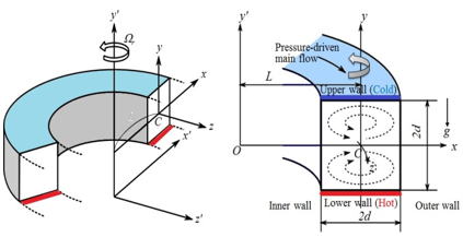
Consider a hydro-dynamically and thermally fully developed two-dimensional (2D) flow of viscous incompressible fluid through a curved square channel, whose height or width is 2d. The coordinate system with relevant notation is shown in Figure 1, where x' and y' axes are taken to be in the horizontal and vertical directions respectively, and z' is the axial direction. It is assumed that the bottom wall of the channel is heated while cooling from the ceiling. The temperature of the bottom wall is $T_{0}+\Delta T$ and that of the top wall $T_{0}-\Delta T$, where $\Delta T>0$. It is also assumed that the flow is uniform in the z' direction and it is driven by a constant pressure gradient G along the centre-line of the channel. Then, the continuity, Navier-Stokes and energy equations, in terms of dimensional variables, are expressed as:
Continuity equation:
$\frac{\partial u^{\prime}}{\partial r^{\prime}}+\frac{\partial v^{\prime}}{\partial y^{\prime}}+\frac{u^{\prime}}{r^{\prime}}=0$ (1)
Momentum equations:
$\frac{\partial u^{\prime}}{\partial t^{\prime}}+u^{\prime} \frac{\partial u^{\prime}}{\partial r^{\prime}}+v^{\prime} \frac{\partial u^{\prime}}{\partial y^{\prime}}-\frac{w^{\prime 2}}{r^{\prime}}=-\frac{1}{\rho} \frac{\partial P^{\prime}}{\partial r^{\prime}}$
$+v\left[\frac{\partial^{2} u^{\prime}}{\partial r^{\prime 2}}+\frac{\partial^{2} u^{\prime}}{\partial y^{\prime 2}}+\frac{1}{r^{\prime}} \frac{\partial u^{\prime}}{\partial r^{\prime}}-\frac{u^{\prime}}{r^{\prime 2}}\right]$ (2)
$\frac{\partial v^{\prime}}{\partial t^{\prime}}+u^{\prime} \frac{\partial v^{\prime}}{\partial r^{\prime}}+v^{\prime} \frac{\partial v^{\prime}}{\partial y^{\prime}}=-\frac{1}{\rho} \frac{\partial P^{\prime}}{\partial y^{\prime}}+v\left[\frac{\partial^{2} v^{\prime}}{\partial r^{\prime 2}}+\frac{1}{r^{\prime}} \frac{\partial v^{\prime}}{\partial r^{\prime}}\right.$
$\left.+\frac{\partial^{2} v^{\prime}}{\partial y^{\prime 2}}\right]+g \beta T^{\prime}$ (3)
$\frac{\partial w^{\prime}}{\partial t^{\prime}}+u^{\prime} \frac{\partial w^{\prime}}{\partial r^{\prime}}+v^{\prime} \frac{\partial w^{\prime}}{\partial y^{\prime}}+\frac{u^{\prime} w^{\prime}}{r^{\prime}}=-\frac{1}{\rho} \frac{1}{r^{\prime}} \frac{\partial P^{\prime}}{\partial z^{\prime}}$
$+v\left[\frac{\partial^{2} w^{\prime}}{\partial r^{\prime 2}}+\frac{\partial^{2} w^{\prime}}{\partial y^{\prime 2}}+\frac{1}{r^{\prime}} \frac{\partial w^{\prime}}{\partial r^{\prime}}-\frac{w^{\prime}}{r^{2}}\right]$ (4)
Energy equation:
$\frac{\partial T^{\prime}}{\partial t^{\prime}}+u^{\prime} \frac{\partial T^{\prime}}{\partial r^{\prime}}+v^{\prime} \frac{\partial T^{\prime}}{\partial y^{\prime}}=\kappa\left[\frac{\partial^{2} T^{\prime}}{\partial r^{\prime 2}}+\frac{1}{r^{\prime}} \frac{\partial T^{\prime}}{\partial r^{\prime}}+\frac{\partial^{2} T^{\prime}}{\partial y^{\prime 2}}\right]$ (5)
where, $r^{\prime}=L+x^{\prime}$, and $u^{\prime}$, $v^{\prime}$ and $w^{\prime}$ are the dimensional velocity components in the x', y' and z' directions respectively and these velocities are zero at the wall. Here, P' is the dimensional pressure, T' is the dimensional temperature and t' is the dimensional time. In the above formulations, $\rho, \mu, \beta, \kappa$ and $g$ are the density, the viscosity, the coefficient of thermal expansion, the coefficient of thermal diffusivity and the gravitational acceleration, respectively. Thus in Eqns. (1) to (5) the variables with prime denotes the dimensional quantities. The dimensional variables are made non-dimensional by using the representative length d, the representative velocity $U_{0}=\frac{v}{d}$, where v is the kinematic viscosity of the fluid. The non-dimensional variables are defined as
$u=\frac{u^{\prime}}{U_{0}}, v=\frac{v^{\prime}}{U_{0}}, w=\frac{\sqrt{2 \delta}}{\mathrm{U}_{\mathrm{o}}} w^{\prime}, x=\frac{x^{\prime}}{d}, \overline{y}=\frac{y^{\prime}}{d}, z=\frac{z^{\prime}}{d}$
$T=\frac{T^{\prime}}{\Delta T^{\prime}}, t=\frac{U_{0}}{d} t^{\prime}, \delta=\frac{d}{L}, P=\frac{P^{\prime}}{\rho U_{0}^{2}}, G=-\frac{\partial P^{\prime}}{\partial z^{\prime}} \frac{d}{\rho U_{0}^{2}}$
where, $\delta$ is the non-dimensional curvature defined as $\delta=\frac{d}{L}$ Since the flow field is uniform in the z-direction, the sectional stream function $\psi$ is introduced as
$u=\frac{1}{1+\delta x} \frac{\partial \psi}{\partial y}$ and $v=-\frac{1}{1+\delta x} \frac{\partial \psi}{\partial x}$ (6)
Figure 1. Coordinate system of the curved channel
Then, the fundamental equations for $w, \cdot \psi$ and T are articulated in terms of non-dimensional variables as
$(1+\delta x) \frac{\partial w}{\partial t}=D n-\frac{\partial(w, \psi)}{\partial(x, y)}+\frac{\delta^{2} w}{1+\delta x}+(1+\delta x) \Delta_{2} w-$
$\frac{\delta}{1+\delta x} \frac{\partial \psi}{\partial y} w+\delta \frac{\partial w}{\partial x}-\delta \operatorname{Tr} \frac{\partial \psi}{\partial y}$ (7)
$\frac{\partial T}{\partial t}+\frac{1}{(1+\delta x)} \frac{\partial(T, \psi)}{\partial(x, y)}=\frac{1}{\operatorname{Pr}}\left(\Delta_{2} T+\frac{\delta}{1+\delta x} \frac{\partial T}{\partial x}\right)$ (8)
$\left(\Delta_{2}-\frac{\delta}{1+\delta x} \frac{\partial}{\partial x}\right) \frac{\partial \psi}{\partial t}=-\frac{1}{(1+\delta x)} \frac{\partial(\Delta \psi, \psi)}{\partial(x, y)}$
$+\frac{\delta}{(1+\delta x)^{2}}\left[\frac{\partial \psi}{\partial y}\left(2 \Delta_{2} \psi-\frac{3 \delta}{1+\delta x} \frac{\partial \psi}{\partial x}+\frac{\partial^{2} \psi}{\partial x^{2}}\right)-\frac{\partial \psi}{\partial x} \frac{\partial^{2} \psi}{\partial x \partial y}\right]$
$+\frac{\delta}{(1+\delta x)^{2}} \times\left[3 \delta \frac{\partial^{2} \psi}{\partial x^{2}}-\frac{3 \delta^{2}}{1+\delta x} \frac{\partial \psi}{\partial x}\right]-\frac{2 \delta}{1+\delta x} \frac{\partial}{\partial x} \Delta_{2} \psi$
$+w \frac{\partial v}{\partial y}+\Delta_{2}^{2} \psi-G r(1+\delta x) \frac{\partial T}{\partial x}+\frac{1}{2} T r \frac{\partial v}{\partial y}$ (9)
The non-dimensional parameters Dn, the Dean number; Gr, the Grashof number; Tr, the Taylor number and Pr, the Prandtl number, which emerge in eqns. (7) to (9) are defined as:
$D n=\frac{G d^{3}}{\mu v} \sqrt{\frac{2 d}{L}}, G r=\frac{\beta g \Delta T d^{3}}{v^{2}}, \operatorname{Pr}=\frac{v}{\kappa}, \operatorname{Tr}=\frac{2 \sqrt{2 \delta} \Omega d^{3}}{v \delta}$ (10)
The stiff boundary conditions for $w$ and $\psi$ are used as
$w( \pm 1, y)=w(x, \pm 1)=\psi( \pm 1, y)=\psi(x, \pm 1)$
$=\frac{\partial \psi}{\partial x}( \pm 1, y)=\frac{\partial \psi}{\partial y}(x, \pm 1)=0$ (11)
and the temperature T is assumed to be constant on the walls as
$T(x, 1)=1, T(x,-1)=-1, T(x, \pm 1)=y$ (12)
There is a group of solutions which satisfy the following symmetry condition with respect to the horizontal plan y=0.
$\left.\begin{array}{l}{w(x, y, t) \Rightarrow w(-x, y, t)} \\ {\psi(x, y, t) \Rightarrow-\psi(-x, y, t)} \\ {T(x, y, t)=-T(-x, y, t)}\end{array}\right\}$ (13)
The solution which satisfies condition (13) is called a symmetric solution, and that does not an asymmetric solution. In the present study, $T r(0 \leq T r \leq 2000)$ and $\delta$$(0.001 \leq \delta \leq 0.5)$ vary while Dn, Gr Pr are fixed as Dn=1000Gr =100 and Pr =7 (water).
3.1 Method of numerical calculation
The present study is based on numerical simulation and in order to attain numerical solution spectral method is used. By this method the variables are expanded in the series of functions consisting of Chebychev polynomials. The expansion functions $\varphi_{n}(x)$ and $\psi_{n}(x)$ are articulated as
$\left.\begin{array}{l}{\varphi_{n}(x)=\left(1-x^{2}\right) \quad C_{n}(x)} \\ {\psi_{n}(x)=\left(1-x^{2}\right)^{2} \quad C_{n}(x)}\end{array}\right\}$ (14)
where, $C_{n}(x)=\cos \left(n \cos ^{-1}(x)\right)$ is the nth order Chebyshev polynomial. $w(x, y, t), \quad \psi(x, y, t)$ and $T(x, y, t)$ are expanded in terms of the expansion functions $\varphi_{n}(x)$ and $\psi_{n}(x)$ as:
$\left.\begin{array}{rl}{w(x, y, t)} & {=\sum_{m=0}^{M} \sum_{n=0}^{N} w_{m n}(t) \phi_{m}(x) \phi_{n}(y)} \\ {\psi(x, y, t)} & {=\sum_{m=0}^{M} \sum_{n=0}^{N} \psi_{m n}(t) \psi_{m}(x) \psi_{n}(y)} \\ {T(x, y, t)} & {=\sum_{m=0}^{M} \sum_{n=0}^{N} T_{m n}(t) \varphi_{m}(x) \varphi_{n}(y)-y}\end{array}\right\}$ (15)
where, M and N are the truncation numbers in the x and y-directions respectively, and $w_{m n}, \psi_{m n}$ and Tmn are the coefficients of expansion. To attain a steady solution $\overline{w}(x, y), \overline{\psi}(x, y)$ and $\overline{T}(x, y)$, the expansion series (15) is put forward into the basic Eqns. (7)-(9) and the collocation method (Gottlieb and Orszag, [29]) is applied. As a result, a set of nonlinear algebraic equations for $w_{m n}, \psi_{m n}$ and Tmn are obtained. The collocation points $\left(x_{i}, y_{j}\right)$ are taken to be
$\left.x_{i}=\cos \left[\pi\left(1-\frac{i}{M+2}\right)\right], y_{j}=\cos \left[\pi\left(1-\frac{j}{N+2}\right)\right]\right\}$ (16)
where, $i=1, \ldots, \quad M+1$ and $j=1, \ldots, \quad N+1$. Steady solutions are obtained by the Newton-Raphson iteration method and to avoid difficulty near the point of inflection for the steady solutions, the arc-length method is used. The arc-length equation is
$\sum_{m=0}^{M} \sum_{n=0}^{N}\left\{\left(\frac{d w_{m n}}{d s}\right)^{2}+\left(\frac{d \psi_{m n}}{d s}\right)^{2}+\left(\frac{d T_{m n}}{d s}\right)^{2}\right\}=1$ (17)
which is solved simultaneously with equation (18) by using the Newton-Raphson iteration method. An initial guess at a point $s+\Delta s$ is considered starting from point s as follows
$\left.\begin{array}{rl}{w_{m n}(s+\Delta s)} & {=w_{m n}(s)+\frac{d w_{m n}(s)}{d s} \Delta s} \\ {w_{m n}(s+\Delta s)} & {=w_{m n}(s)+\frac{d w_{m n}(s)}{d s} \Delta s} \\ {T_{m n}(s+\Delta s)} & {=T_{m n}(s)+\frac{d T_{m n}(s)}{d s} \Delta s}\end{array}\right\}$ (18)
The convergence is assured by taking suitably small $\varepsilon_{p}$ $\left(\varepsilon_{p}<10^{-10}\right)$ defined as
$\varepsilon_{p}=\sum_{m=0}^{M} \sum_{n=0}^{N}\left[\begin{array}{c}{\left(w_{m}^{(p+1)}-w_{m n}^{p}\right)^{2}+\left(\psi_{m n}^{(p+1)}-\psi_{m n}^{p}\right)^{2}} \\ {+\left(T_{m n}^{(p+1)}-T_{m n}^{p}\right)^{2}}\end{array}\right]$ (19)
To solve the steady solution, time-derivative terms are set to zero and the expansion series (15) with coefficients $w_{m n}, \psi_{m n}$ and $T_{m n}$, being time independent, is substituted into the basic Equations (7), (8) and (9). Finally, in order to calculate the trembling solutions, the Crank-Nicolson and Adams-Bashforth methods together with the function expansion (15) and the collocation methods are applied to equations (7) - (9).
3.2 Numerical accuracy
The accuracy of the numerical calculations is investigated for the truncation numbers M and N used in this study. For good accuracy of the solutions, N is chosen equal to M. Table 1 shows that M=20 and N=20 give sufficient accuracy of the present numerical solutions.
Table 1. The values of Q and $w(0,0)$ for various M and N at Dn=1000, Gr=100, Tr=1000 and $\delta=0.001$
|
M |
N |
Q |
$w(0,0)$ |
|
16 |
16 |
269.1777139229 |
385.99227522622 |
|
18 |
18 |
270.0915731736 |
385.49012540331 |
|
20 |
20 |
270.1417120204 |
385.05629891693 |
|
22 |
22 |
270.1948353760 |
384.88687539512 |
3.3 Flux through the channel
In the present study, the dimensional total flux Q' through the channel in the rotating coordinate system is expressed by
$Q^{\prime}=\int_{-d}^{d} \int_{-d}^{d} w^{\prime} d x^{\prime} d y^{\prime}=V d Q$ (20)
where, dimensionless total flux Q is defined as,
$Q=\int_{-1}^{1} \int_{-1}^{1} w d x d y$ (21)
The mean axial velocity $\overline{w^{\prime}}$ is calculated by
$\overline{w^{\prime}}=\frac{Q v}{4 d}$ (22)
In this paper, Q is used to designate the steady solution branches and to pursue the time evolution of the tremulous solutions.
4.1 Steady solution
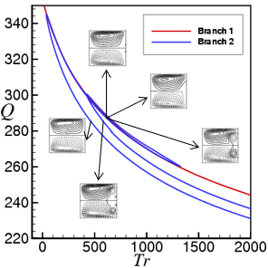
In this study, we first investigate solution structure of the steady solutions for curvature $\delta=0.001$ and discuss the pattern distinction of secondary flows on various branches of steady solutions and then summarize the solutions for other curvatures. After an extensive appraisal over the parametric ranges, two branches of steady solutions are achieved for Dn=1000 and Gr=1000 over $0 \leq \operatorname{Tr} \leq 2000$. A bifurcation diagram of steady solutions is shown in Figure 2 for $\delta=0.001$ using Q, the representative quantity of the flow state. The two steady solution branches are named the first steady solution branch (1st branch, red solid line) and the second steady solution branch (2nd branch, blue solid line), respectively. The solution branches are obtained by the path continuation technique with various initial guesses and are distinguished by the nature and number of secondary vortices appearing in the cross-section of the channel. It is found that the branches are independent and there exists no bifurcating connection between the two branches.
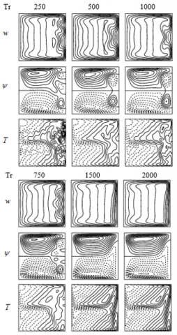
Figure 3 shows streamlines and isotherms for various values of Tr. In the following, the two branches of steady solutions and flow patterns on respective branches are discussed in brief.
Figure 2. Solution structure of steady solutions for $\delta=0.001$, Dn=1000, Gr=1000 and $0 \leq \operatorname{Tr} \leq 2000$
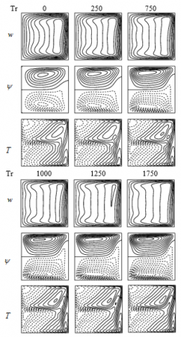
Figure 3. Streamlines of axial flow (top), secondary flow (middle) and isotherm (bottom) on the steady solution branches for various values of Tr
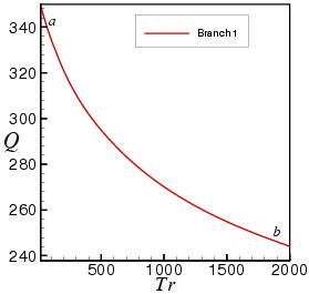
The first steady solution branch for $\delta=0.001$ is shown explicitly in Figure 4 by red solid line for $(0 \leq T r \leq 2000)$. The branch starts at point ‘a’ $(T r=0)$ and goes to the direction of increasing Tr up to point ‘b’(Tr=2000) without any turning. Figure 5 shows streamlines of axial flow, secondary flow and isotherm (temperature contour) on the first steady solution branch at various values of Tr. To draw the contours of $w, \psi$ and $T$, we use the increment $\Delta w=8.0$, $\Delta \psi=0.9 \quad$ and $\quad \Delta T=0.15$ respectively. The solid lines $(\psi \geq 0, T \geq 0)$ show that the secondary flow is in the clockwise direction whiles the dotted ones $(\psi<0, T<0)$ in the counter clockwise direction.
As seen in Figure 5, the 1st branch consists of asymmetric two-vortex solution. It is found that the streamlines of the secondary flow consist of two opposite vortices; one is an outward flow (anticlockwise direction) shown by solid line and the other inward flow (clockwise direction) shown by dotted lines. The flow is accelerated due to combined action of the centrifugal, Coriolis and buoyancy forces; centrifugal force is created due to the motion through a curved channel, Coriolis force due to the rotation of the channel around the vertical axis while buoyancy forces because of the thermal gradient.
Figure 4. First steady solution branch for $\delta=0.001$, Dn=1000, Gr=1000 and $0 \leq \operatorname{Tr} \leq 2000$
Figure 5. Streamlines of axial flow (top), secondary flow (middle) and isotherm (bottom) on the 1st branch for various values of Tr at for $\delta=0.001$
4.1.2 The second steady solution branch
The second steady solution branch, designated by the blue solid line, is exclusively shown in Figure 6(a). It is found that the branch is a little bit entangled experiencing many turnings on its way. The branch starts at point ‘a’(Tr=2000) and finally arrives at point ‘g’ with turnings at points b, c, d, e and f. It is found that the branch turns very smoothly at points b (Tr=35.90), c (Tr=1318.29) , d (Tr=421.96) , e (Tr=672.41) and at point f (Tr=658.45) before arriving finally at point g (Tr=2000) . It is fascinating that the branch starts with two-vortex solution at the starting point a (Tr=2000) and lastly turns into eight-vortex solution at points e, f and g. Enlargements at points b, c, d, e and f are shown in Figures 6(b), 6(c), 6(d) and 6(e) respectively. Figure 7 shows streamlines of axial flow, secondary flow and isotherms on the 2nd branch for $\delta=0.001$, Dn=1000, Gr=100. As seen in Figure 7, the branch is composed of two- to eight-vortex solution. It is found that as soon as the branch turns at a point, the number of secondary vortices increases, for example, two-vortex solution turns into four-vortex; four-vortex into six-vortex and finally six-vortex into eight-vortex solution. In this study, temperature profiles show that the streamlines of the temperature distribution are uniformly distributed to all parts of the contour transferring heat from outer wall to the fluid, and the contribution of the rotation and pressure on secondary flows significantly change and increase the number of secondary vortices. It is clearly evident that heating the bottom wall causes the temperature contours to become asymmetrical in comparison to isothermal cases. This essentially arises from the interaction between the heating-induced buoyancy force and the centrifugal force that drives secondary vortices. In this regard, it should be noted that the centrifugal force due to the channel curvature creates two effects; one is a positive radial fluid pressure field in the duct cross-section and induces a lateral fluid motion driven from inner wall towards the outer wall. This lateral fluid motion occurs against the radial pressure field generated by the centrifugal effect and is superimposed on the axial flow to create the secondary vortex flow structure. As the flow through the channel is increased, the lateral fluid motion becomes stronger and the radial pressure field is intensified. In the vicinity of the outer wall, the combined action of adverse radial pressure field and viscous effects slows down the lateral fluid motion and forms an inactive flow region. Beyond a certain critical value of Dn, the radial pressure gradient becomes sufficiently strong to reverse the flow direction of the lateral fluid flow. A weak local flow re-circulation is then established creating an additional pair of vortices in the stagnant region near the outer wall. This flow condition is known as Dean’s hydrodynamic instability while the vortices are termed as Dean vortices.
Figure 6. (a) Second steady solution branch, (b) Enlargement at point b, (c) Enlargement at point c, (d) Enlargement at point d, and, (e) Enlargements at points e and f
Figure 7. Streamlines of axial flow (top), secondary flow (middle) and isotherm (bottom) on the first steady solution branch for various values of Tr
4.2 Linear stability analysis
In this study, linear stability of the steady solutions is investigated against only 2D perturbations (z-independent). For this purpose, the eigenvalue problem is solved by application of the function expansion method together with collocation method to the linearized equations for the perturbation of $\overline{w}(x, y), \overline{\psi}(x, y)$ and $\overline{T}(x, y)$. It is assumed that the time dependence of the perturbation is $e^{\sigma t}$, where $\sigma=\sigma_{r}+i \sigma_{i}$. If all the real parts $\sigma_{r}$ of the eigenvalue $\sigma$ are negative, the steady solution is linearly stable, but if there exist at least one positive real part, it is linearly unstable. In the unstable region, the perturbation grows monotonically for $\sigma_{i}=0$ and oscillatory for $\sigma_{i} \neq 0$. In this study, it is found that between the two branches of steady solutions, only the 2nd branch is linearly stable for a small region of Tr $(164.82 \leq T r \leq 601.62)$ while unstable otherwise. The stability result is shown in Table 2, where linearly stable solutions are shown with bold. Linear stability region is shown with solid thick line in Figure 8.
Table 2. Linear stability of the 2nd branch for $\delta=0.001$, Dn=1000 and Gr=100 for various values of Tr
|
Tr |
Q |
$\sigma_{r}$ |
$\sigma_{i}$ |
|
2000 |
231.0515886 |
225.86 |
0 |
|
1500 |
241.7277581 |
191.77 |
0 |
|
1000 |
270.0175071 |
13.032 |
$-1.0693 \times 10^{2}$ |
|
601.63 |
287.9733094 |
$2.4732 \times 10^{-4}$ |
$-7.6900 \times 10^{2}$ |
|
601.62 |
287.9738766 |
$-4.0767 \times 10^{-5}$ |
$-7.6899 \times 10$ |
|
164.82 |
325.4912274 |
$-8.9249 \times 10^{-4}$ |
$-2.2273 \times 10$ |
|
164.81 |
325.4926111 |
$6.5622 \times 10^{-4}$ |
$2.2270 \times 10$ |
|
35.90 |
344.8927460 |
5.0054 |
0 |
Figure 8. Linear stability region (solid black line) on the 2nd branch for $\delta=0.001$
4.3 Time-dependent solutions
4.3.1 Time-evolution calculation of the unsteady solution for $\delta=0.001$
We investigate time-dependent solutions for the curvatures ranging from 0.001 to 0.5 but here we show the detailed unsteady results for $\delta=0.001$ only and then summarize the complete solutions at the end of this section.
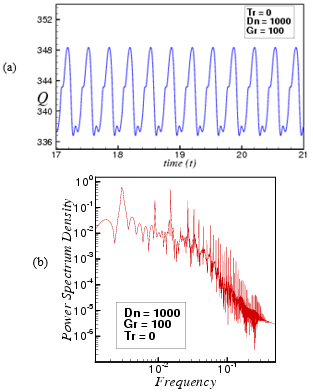
Figure 9. (a) Time history of Q for $T r=0$ (b) Power spectrum density
In order to examine non-linear behavior of the unsteady solutions, we performed time history of Q for Tr=0 at $\delta=0.001$ as shown in Figure 9(a) in the t-Q plane. It is found that the time-dependent flow at Tr=0 is a multi-periodic oscillation. To well justify the multi-periodic flow more evidently, we obtained power spectrum density of the time-evolution result as shown in Figure 9(b) in the Frequency vs. Power Spectrum Density plane. Figure 9(b) shows that not only the line spectrum of the fundamental frequency and its harmonics but other line spectrum and their harmonics are seen with small amplitudes, which shows that the oscillation presented in Figure 9(a) is multi-periodic. To monitor vortex-structure and temperature distribution, we obtain streamlines of axial flow and secondary flow and isotherm as shown in Figure 10 for C . It is found that secondary flow is an asymmetric two- to four-vortex solution. It is also found that the maximum axial velocity is gathered near the outer wall of the channel.
Figure 10. Streamlines of axial flow (top) and secondary flow (middle) and isotherm (bottom) for Tr=0 at $19.00 \leq t \leq 19.65$
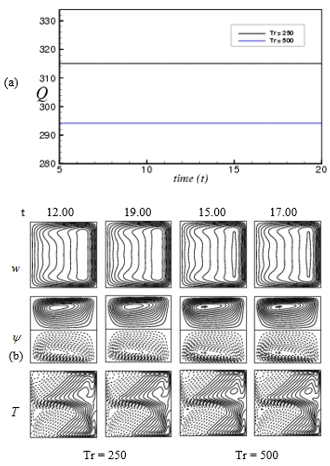
Then we inspect time history for Tr=250 and 500 as shown in Figure 11 (a). It is found that the time-dependent flow for Tr=250 and 500 is a steady-state solution which is consistent with the linear stability results presented in Section 4.2, where we obtained that the flow is steady-stable for $164.82 \leq T r \leq 601.62$. Since the flow is steady-state, a single contour of each of the axial flow, secondary flow and temperature profile is shown in Figure 11 (b) for Tr=250 and 500 . It is found that steady-state flow is an asymmetric two-vortex solution.
Figure 11. (a) Time history of Q and $\delta=0.001$ (b) Streamlines of axial flow (top) and secondary flow (middle) and isotherm (bottom) for Tr=250 and 500
Figure 12. (a) Time history of Q for Tr=750 (b) Power spectrum density
We then performed time-history of Q for Tr=750 as shown in Figure 12(a) and it is found that the time-dependent flow for Tr=750 is a time-periodic flow. In order to see the flow evolution more precisely we also obtain power spectrum density of the time change of Q as shown in Figure 12(b), which shows that only the line spectrum of the fundamental frequency and its harmonics are seen which pointed out that the flow is time periodic for Tr = 750. Streamlines and isotherms Tr=750 are shown in Figure 13 for one period of oscillation at $33.05 \leq t \leq 33.55$, and it is found that the periodic flow oscillates between asymmetric two-vortex solution. The transition from steady-state to periodic oscillation takes place between Tr=750 and Tr=750 . In fact, the periodic oscillation, which is observed in the present study, is a traveling wave solution advancing in the downstream direction which was well-justified by Mees et al. [30] and Wang and Yang [19] and in the recent investigation by Yanase et al. [31] for three-dimensional travelling wave solutions as an appearance of 2D periodic oscillation.
Figure 13. Streamlines of axial flow (top) and secondary flow (middle) and isotherm (bottom) for Tr=750 at $33.05 \leq t \leq 33.55$
Figure 14. (a) Time history of Q for Tr=1000 (b) Power spectrum density
If the rotational speed is increased, it is observed that the flow characteristics change. Figures 14(a) and 16(a) respectively show time history of Q for Tr=1000 and Tr=1250 and it is seen that the flow oscillates irregularly that means the flow is chaotic. With a view to observing the chaotic behavior more explicitly, power spectrum density of the time change of Q are shown in Figures 14(b) and 16(b) for Tr=1000 and Tr=1250 respectively, and it is found that continuous line spectrum with different frequencies are available for these cases, which shows that the flow is chaotic for Tr=1000 and Tr=1250 . This type of flow evolution is termed as weak chaos [6]. To detect the change of the irregular oscillations, typical contours of streamlines and isotherms for Tr=1000 and Tr=1250 are shown in Figures 15 and 17 respectively and it is found that the chaotic flow at Tr=1000 and Tr=1250 oscillates between asymmetric two-vortex solutions.
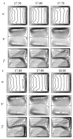
Figure 15. Streamlines of axial flow (top) and secondary flow (middle) and isotherm (bottom) for Tr=1000 at $17.50 \leq t \leq 18.00$
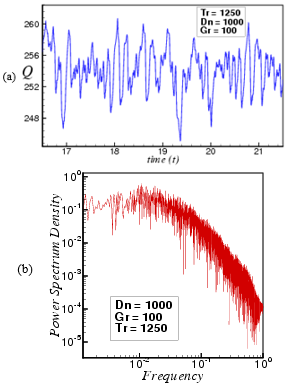
Figure 16. (a) Time history of Q for Tr=1250, (b) Power spectrum density
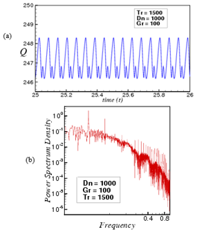
If Tr is increased further, for example Tr=1500, we see that the flow development changes and it becomes multi-periodic. By the time history analysis we obtained multi-periodic solution for Tr=1500 as shown in Figure 18 (a). To observe the multi-periodic oscillation more clearly, we calculated power spectrum density of the time change of Q as shown in Figure 18 (b), which shows that not only the line spectrum of the fundamental frequency and its harmonics but other line spectrum of smaller frequencies and their harmonics are seen, which indicates that the flow presented in Figure 18(a) is multi-periodic. Then with a view to observing the configuration of axial and secondary vortices along with temperature distributions for the multi-periodic oscillation at Tr=1500 , typical contour of the streamlines and isotherms are shown in Figure 19 for Tr=1500 and it is found that the time-dependent solution at Tr=1500 oscillates between two- to three-vortex solutions. From Figures 13 and 14, it is clear that the transition from chaotic state to multi-periodic oscillation occurs between Tr=1200 and Tr=1500.
Then, time history of Q for Tr=1750 and Tr=2000 are obtained as shown in Figures 20 (a) & 22 (a) respectively. It is found that the flow oscillates irregularly with large windows of quasi-periodic oscillations that mean the flow is chaotic. This chaotic oscillation is well justified by drawing the power spectrum density of the solutions as show in Figures 20 (b) and 22 (b) respectively. Figures 20 (b) & 22 (b) show that continuous line spectrum with dissimilar frequencies cover the Frequency vs. Power spectrum Density plane so that the flow presented in Figures 20 (a) & 22 (a) are strongly chaotic for Tr=1750 and Tr=2000 respectively. This type of flow oscillation is termed as strong chaos [6]. Thus illustration the power spectrum of the solutions is found to be very fruitful to well justify the flow distinctiveness as well as identifying the transition of the time-dependent solutions from one state to another.
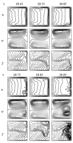
Figure 17. Streamlines of axial flow (top) and secondary flow (middle) and isotherm (bottom) for Tr=1250 at $19.45 \leq t \leq 19.95$
Figure 18. (a) Time history of Q for Tr=1500, (b) Power spectrum density
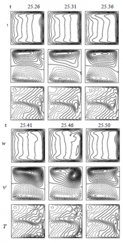
Figure 19. Streamlines of axial flow (top) and secondary flow (middle) and isotherm (bottom) for Tr=1500 at $25.26 \leq t \leq 25.50$
Figure 20. (a) Time history of Q for Tr=1750, (b) Power spectrum density
Figure 21. Streamlines of axial flow (top) and secondary flow (middle) and isotherm (bottom) for Tr=1750 at $27.00 \leq t \leq 27.50$
Figure 22. (a) Time history of Q for Tr=2000, (b) Power spectrum density
To scrutinize the pattern variation of axial and secondary vortices and isotherms of the temperature distributions for the chaotic oscillation, typical contours of axial flow distribution, secondary flow patterns and temperature profiles are shown in Figures 21 & 23 for Tr=1750 and Tr=2000 respectively, and it is found that the time-dependent solutions oscillate erratically in the two- to six-vortex solutions. These vortices are produced due to combined action of the centrifugal, Coriolis and buoyancy forces. In this study, it is found that the number of secondary vortices increases for the chaotic solution, which occurs at large Tr’s compared to that of the steady-state or periodic solutions at small Tr, and consequently it is suggested that chaotic solutions enhance heat transfer more effectively than the steady-state or periodic solutions. In this regard, it should be noted that, the occurrence of the chaotic state, as presented in the present study, is related to the destabilization of the periodic or quasi-periodic solutions which reminds us the case of Lorenz attractor [32]. It may be promising that the transition in the present study is caused by a similar mechanism as that of Ruelle-Takens scenario [33] in the laminar flow. In this study, it is very interesting to notice that the flow is symmetrically distributed and the vortices are formed very close to the wall and rests of the streamlines are not affected by the Dean vortices. It is observed that the number of secondary vortices increase (six- to eight-vortex solution) for chaotic flow which occurs at large Tr, and reached at the highest number compared with those obtained at small Tr. As Tr increases, the fluid particles move in the vicinity of the wall and make friction to each other; at a certain time, Dean vortices are constructed yonder the wall of the channel which plays an outstanding responsibility in transferring heat from the heated bottom wall to the fluid.
Figure 23. Streamlines of axial flow (top) and secondary flow (middle) and isotherm (bottom) for Tr=2000 at $19.00 \leq t \leq 20.00$
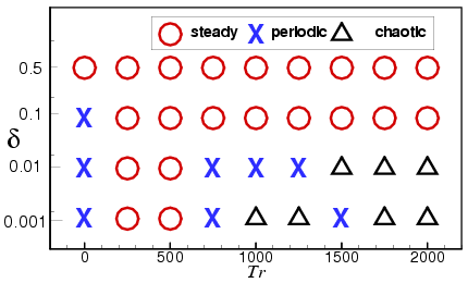
4.3.2 Time-dependent solutions in $(\operatorname{Tr}-\delta)$ plane
In this sub-section, the distribution of the steady, periodic (or multi-periodic) and chaotic solutions, obtained by the time-evolution calculations, is presented in Figure 24 in the Taylor number vs. curvature $(\operatorname{Tr}-\delta)$ plane for $0<\operatorname{Tr} \leq 2000$ and $0.001 \leq \delta \leq 0.5$. In this picture, the circle indicates steady-state solutions, the cross periodic (or multi-periodic) solutions and the triangle chaotic solutions. It is found that at $\delta=0.001$, chaotic behavior is established in the middle of two periodic oscillation for $950 \leq \operatorname{Tr} \leq 1300$ whereas the chaotic behavior is converted into periodic oscillation between the required range of $\operatorname{Tr}(950 \leq \operatorname{Tr} \leq 1300)$ at $\delta=0.01$. A drastic change is observed in the unsteady flow characteristics from curvature $\delta=0.01$ to $\delta=0.1$. It is found that the chaotic behavior is totally diminished at $\delta=0.1$ and periodic oscillation is found for a small range of $\operatorname{Tr}(0 \leq \operatorname{Tr} \leq 239)$ where the steady-state behavior is found for a wide range of $T r$, and for $\delta=0.5$ only steady-state solution is observed. It is, therefore, evident that as curvature is increased, the oscillating behavior in the rotating curved channel is decreased and the flow ceases to be steady-state.
Figure 24. Time-dependent solutions for $0.001 \leq \delta \leq 0.5$ at $D n=1000$ and $G r=100$
4.3.3 Vortex diagram in Taylor number vs. curvature $(T r-\delta)$ plane
In this section, to observe vortex-structure of secondary flows, we show pattern variation of secondary flows for different values of Tr . Figure 25 shows vortex structure of secondary flows for $D n=1000 \quad$ and $\quad 0 \leq \operatorname{Tr} \leq 2000$ for curvature $0.001 \leq \delta \leq 0.5$, where it is found that the secondary flow is a two- to eight-vortex solution at various values of Tr . It is found that maximum 8-vortex solution is attained at the small curvature $\delta=0.001$, while four- and two-vortex for moderate and strong curvatures at $\delta=0.1 \quad$ and $\quad \delta=0.5$ respectively. It is found that the number of secondary vortices decreases as Tr increases. In this study, it has been found that for the unsteady case dual solutions (two-vortex solution) exist for the steady-state solution, two- to four-vortex for the periodic solution while two- to six-vortex for the chaotic solution. Therefore, it is recommended that chaotic solutions intensify heat transfer more effectively than the periodic or steady-state solution; this is because many secondary vortices are produced at the outer concave wall for the chaotic solution. In this regard, it should be noted that very recently, Razavi et al. [27] employed control volume method to investigate flow characteristics, heat transfer and entropy generation in a rotating curved duct. The effects of Dean number, wall heat flux and force ratio on the entropy generation were presented in that paper. However, solution structure of steady solutions as well as complete behavior of the unsteady solutions with flow transition is still absent in literature for rotating curved duct flows; which has been described in the present paper very clearly. Furthermore, hydrodynamic instability and vortex generation, which is presented in the present paper, gives a clear view about the convective heat transfer in a curved duct via periodic, multi-periodic and chaotic flows. As of now, a reliable technique for Dean instability is not known in literature for such flows. The present study also shows that there is a strong interaction between the heating-induced buoyancy force and the centrifugal-Coriolis instability in the curved channel that stimulates fluid mixing and thus results in thermal enhancement in the flow, because heated fluid is transported into the bulk fluid by the secondary vortices; this process is preciously demonstrated by the temperature contours as shown in the present study.
Figure 25. Vortex diagram of secondary flows for $0.001 \leq \delta \leq 0.5$ at $D n=1000$ and $G r=100$
4.4 Convective heat transfer
In order to investigate convective heat transfer from the heated wall to the fluid, we calculate temperature gradients at the cooling (bottom) and heated (top) walls. As seen in Figure 26 (a), the temperature gradient on the bottom (heated) wall, $\frac{\partial T}{\partial x}$ increases at the central region through the small vibration of the heating wall by increasing and decreasing. This is because the secondary flow enhances $\frac{\partial T}{\partial x}$ not only in the central region but in other regions as well. In Figure 26 (b), on the other hand, it is found that $\frac{\partial T}{\partial x}$ on the top (cooled) wall decreases in the central region around y = 0. This is caused by the advection of the secondary flow in the outward direction around y = 0 due to the centrifugal force. In the same figure, it is also shown that $\frac{\partial T}{\partial x}$ tends to increase in the regions other than the central region. This is caused by the advection of the secondary flow in the inward direction there, which is a reverse flow of the outward secondary flow in the central region. This result shows that heat transfer occurs substantially from the heated wall to the fluid as Tr increases.
Figure 26. Temperature gradients, (a) At the heated (bottom) wall, (b) At the cooling (top) wall at various values of Tr
4.5 Validation of the numerical result
Figure 27. Experimental vs. numerical results for rotating curved square channel flow at Tr = 150. (a), (b) & (c) Experimental result by Yamamoto et al. [21] (left) and numerical result by the authors (right)
Here, we will discuss the validity of our numerical results with the experimental studies conducted by some authors. By using visualization method, Yamamoto et al. [21] performed experimental investigations of the flow through a rotating curved square duct of curvature d = 0.03, where three of the duct walls, except the outer wall, rotate around the center of curvature at a constant rotational speed for positive rotation (Tr =150) of the duct walls. In the present study, however, we investigate flow characteristics for rotating the whole system (not the three walls only), and to show the validity of the present study we use the same curvature and Tr as Yamamoto et al. [21] used. Figures 27 (a), (b), (c) and (d) show comparative study of the experimental vs. numerical results for the rotating curved square channel flow at different values of Dn for the rotational parameter, Tr = 150. As seen in Figure 27, our numerical results have a good agreement with the experimental investigations obtained by Yamamoto et al. [21].
In this paper, a spectral-based numerical study is presented for fluid flow and heat transfer through a rotating curved square channel of curvature $0.001 \leq \delta \leq 0.5$ over a wide range of positive rotation of the channel for $0 \leq \operatorname{Tr} \leq 2000$ for constant Dean number Dn=100. The bottom wall of the channel is heated while cooling from the ceiling. After an extensive survey over the range of the parameters, two branches of asymmetric steady solutions are obtained for with no bifurcating relationship between the branches. Linear stability analysis shows that only the second branch is linearly stable for $601.62 \leq T r \leq 164.82$ and unstable otherwise. In the unstable region, time-history analysis as well as power spectrum density show that the flow undergoes through various flow instabilities in the scenario “multi-periodic $\rightarrow$ steady-state $\rightarrow$ periodic $\rightarrow$ chaotic $\rightarrow$ multi-periodic $\rightarrow$ chaotic”, if Tr is increased in the positive direction. Typical contours of streamlines and isotherms are obtained at a number of values of Tr, and it is found that there exist two- to eight-vortex for the steady-state solution, two- to four-vortex for the periodic or multi-periodic solution while two- to eight-vortex for the chaotic solution. It is observed that the number of secondary vortices increases as the flow becomes chaotic propagating multi-vortex solutions at the outer concave wall and consequently it is disclosed that chaotic solutions enhance heat transfer more effectively than the steady-state or periodic solutions. It is also concluded that the temperature contour is coherent with the secondary vortices, and secondary flows play an effective role in transferring heat from the heated bottom wall to the fluid. The results clearly show the existence of multiple Dean vortices along the duct and both axial velocity and wall pressure is greatly influenced by the Dean vortices. The present investigation also shows that there is a strong interaction between the heating-induced buoyancy force and the centrifugal-Coriolis instability in the rotating curved channel that stimulates fluid mixing and therefore increases heat transfer in the fluid. Finally, our numerical results are compared with the experimental investigations, and it is found that there is a good agreement between the numerical and experimental investigations.
"Rabindra Nath Mondal, one of the authors, would gratefully acknowledge the financial support from the Bangladesh Ministry of Education (MoEdu) for advanced research in science and Technology, No. 37.20.0000.004.033.005.2014-1309/1(42), to conduct this research work".
|
Dn |
Dean number |
|
|
Gr |
Grashof number |
|
|
Pr |
Prandtl number |
|
|
a |
Aspect ratio |
|
|
L |
Radius of the curvature |
|
|
x |
Horizontal axis |
|
|
y |
Vertical axis |
|
|
z |
Axis in the direction of the main flow |
|
|
u |
Velocity components in the x- direction |
|
|
v |
Velocity components in the y- direction |
|
|
w |
Velocity components in the z- direction |
|
|
T |
Temperature |
|
|
t |
Time |
|
|
Greek symbols
|
||
|
$\delta$ |
Curvature of the duct |
|
|
$\rho$ |
Density |
|
|
$\lambda$ |
Resistance coefficient |
|
|
$\mu$ |
Viscosity |
|
|
$\boldsymbol{\kappa}$ |
Thermal diffusivity |
|
|
$v$ |
Kinematic viscosity |
|
|
$\psi$ |
Sectional stream function |
|
[1] Dean, W.R. (1927). Note on the motion of fluid in a curved pipe. Philos Mag., 4: 208-23. https://doi.org/10.1080/14786440708564324
[2] Berger, S.A., Talbot, L., Yao, L.S. (1983). Flow in curved pipes. Annual. Rev. Fluid. Mech., 35: 461-512. https://doi.org/10.1146/annurev.fl.15.010183.002333
[3] Nandakumar, K., Masliyah, J.H. (1986). Swirling flow and heat transfer in coiled and twisted pipes. Advanced Transport Process, 4: 49-112.
[4] Zhang, J.S., Zhang, B.Z., Ju, J. (2001). Fluid flow in a rotating curved rectangular duct. International Journal of Heat and Fluid Flow, 22: 583-592. https://doi.org/10.1016/S0142-727X(01)00126-6
[5] Yanase, S., Kaga, Y., Daikai, R. (2002). Laminar flow through a curved rectangular duct over a wide range of aspect ratio. Fluid Dynamics Research, 31: 151-83. https://doi.org/10.1016/S0169-5983(02)00103-X
[6] Mondal, R.N., Kaga, Y., Hyakutake, T., Yanase, S. (2007). Bifurcation diagram for two-dimensional steady flow and unsteady solutions in a curved square duct. Fluid Dynamics Research, 39: 413-446. https://doi.org/10.1016/j.fluiddyn.2006.10.001
[7] Cheng, K.C., Lin, R.C., Ou, J.W. (1975). Graetz problem in curved square channels. Journal of Heat Transfer, 97: 244-248. https://doi.org/10.1115/1.3450348
[8] Shantini, W., Nandakumar, K. (1986). Bifurcation phenomena of generalized Newtonian fluids in curved rectangular ducts. Journal of Non-Newtonian Fluid Mechanics, 22: 35-60. https://doi.org/10.1016/0377-0257(86)80003-9
[9] Finlay, W.H., Nandakumar, K. (1990). Onset of two dimensional cellular flow in finite curved channels of large aspect ratio. Physics of Fluids, A2: 1163-1174. https://doi.org/10.1063/1.857617
[10] Thangam, S., Hur, N. (1990). Laminar secondary flows in curved rectangular ducts. Journal of Fluid Mechanics, 217: 421-440. https://doi.org/10.1017/S0022112090000787
[11] Selmi, M., Namadakumar, K., Finlay, W.H. (1994). A bifurcation study of viscous flow through a rotating curved duct. Journal of Fluid Mechanics, 262: 353-375. https://doi.org/10.1017/S0022112094000534
[12] Dennis, S.C.R., Ng, M. (1982). Dual Solutions for steady laminar flow through a curved tube. Q J. Mech. Appl. Math., 99: 449-67. https://doi.org/10.1093/qjmam/35.3.305
[13] Winters, K.H. (1987). A bifurcation study of laminar flow in a curved tube rectangular cross section. Journal of Fluid Mechanics, 180: 343-369. https://doi.org/10.1017/S0022112087001848
[14] Hasan, M.S., Islam, M.M., Ray, S.C., Mondal, R.N. (2019). Bifurcation structure and unsteady solutions through a curved square duct with bottom wall heating and cooling from the ceiling. AIP Conference Proceedings 2121, 050003. https://doi.org/10.1063/1.5115890
[15] Chandratilleke, T.T, Nadim, N., Narayanaswamy, R. (2012). Vortex structure-based analysis of laminar flow behavior and thermal characteristics in curved ducts. Int. J. Thermal Sci., 59: 75-86. https://doi.org/10.1016/j.ijthermalsci.2012.04.014
[16] Wu, X.Y., Lai, S.D., Yamamoto, K., Yanase, S. (2013). Numerical analysis of the flow in a curved duct. Advanced Materials Research, 706-708: 1450-1453. https://doi.org/10.4028/www.scientific.net/AMR.706-708.1450
[17] Li, Y., Wang, X., Zhou, B., Yuan, S., Tan, S.K. (2017). Dean instability and secondary flow structure in curved rectangular ducts. Int. J. Heat and Fluid Flow, 68: 189-202. https://doi.org/10.1016/j.ijheatfluidflow.2017.10.011
[18] Yanase, S., Nishiyama, K. (1988). On the bifurcation of laminar flows through a curved rectangular tube. J. Phys. Soc. Jpn., 57(11): 3790-5. https://doi.org/10.1143/JPSJ.57.3790
[19] Wang, L., Yang, T. (2005). Periodic oscillation in curved duct flows. Physica D, 200: 296 -302. https://doi.org/10.1016/j.physd.2004.11.003
[20] Hasan, M.S., Mondal, R.N., Kouchi, T., Yanase, S. (2019). Hydrodynamic instability with convective heat transfer through a curved channel with strong rotational speed. AIP Conference Proceedings 2121, 030006. https://doi.org/10.1063/1.5115851
[21] Yamamato, K., Xiaoyum, W., Kazou, N., Yasutuka, H. (2006). Visualization of Taylor-Dean flow in a curved duct of square cross section. J. Fluid Dyn. Res., 38: 1-18. https://doi.org/10.1016/j.fluiddyn.2005.09.002
[22] Liu, F., Wang, L. (2009). Analysis on multiplicity and stability of convective heat transfer in tightly curved rectangular ducts. Int. J. Heat and Mass Transfer, 52: 5849-5866. https://doi.org/10.1016/j.ijheatmasstransfer.2009.07.019
[23] Mondal, R.N., Islam, M.S., Uddin, M.K., Hossain, M.A. (2013). Effects of aspect ratio on unsteady solutions through a curved duct flow. Appl. Math. & Mech., 34(9): 1-16. https://doi.org/10.1007/s10483-013-1731-8
[24] Li, Y., Wang, X., Yuan, S., Tan, S.K. (2016). Flow development in curved rectangular ducts with continuously varying curvature. Experimental Thermal and Fluid Science, 75: 1-15. https://doi.org/10.1016/j.expthermflusci.2016.01.012
[25] Chandratilleke, T.T., Nursubyakto. (2003). Numerical prediction of secondary flow and convective heat transfer in externally heated curved rectangular ducts. Int. J. Thermal Sci., 42(2): 187-198. https://doi.org/10.1016/S1290-0729(02)00018-2
[26] Norouzi, M., Kayhani, M.H., Nobari, M.R.H., Demneh, M.K. (2009). Convective heat transfer of viscoelastic flow in a curved duct. World Acad. Sci. Eng. Tech., 32: 327-33.
[27] Razavi, S.E., Soltanipour, H., Choupani, P. (2015). Second law analysis of laminar forced convection in a rotating curved duct. Thermal Sciences, 19(1): 95-107. https://doi.org/10.2298/TSCI120606034R
[28] Zhang, W., Wei, Y., Dou, H.S., Zhu, Z. (2018). Transient behaviors of mixed convection in a square enclosure with an inner impulsively rotating circular cylinder. International Communications in Heat and Mass Transfer, 98: 143-154. https://doi.org/10.1016/j.icheatmasstransfer.2018.08.016
[29] Gottlieb, D., Orazag, S.A. (1977). Numerical analysis of spectral methods. Society of Industrial and Applied Mathematics, Philadelphia, USA. https://doi.org/10.1137/1.9781611970425
[30] Mees, P.A.J, Nandakumar, K., Masliyah, J.H. (1996). Instability and transitions of flow in a curved square duct: the development of the two pairs of dean vortices. J. Fluid Mech., 314: 227-46. https://doi.org/10.1017/S0022112096000298
[31] Yanase, S., Watanabe, T., Hyakutake, T. (2008). Traveling-wave solutions of the flow in a curved-square duct. Physics of Fluids, 20(124101): 1-8. https://doi.org/10.1063/1.3029703
[32] Lorenz, E.N. (1963). Deterministic non-periodic flow. J. Atoms Sci., 20: 130-141. https://doi.org/10.1175/1520-0469(1963)020<0130:DNF>2.0.CO;2
[33] Ruelle, D., Takens, F. (1971). On the nature of turbulence. Commun Math Phys., 20: 167-92. https://doi.org/10.1007/BF01646553