Rafael da Silveira Borahel* | Rejane de Césaro Oliveski | Ligia Damasceno Ferreira Marczak
© 2019 IIETA. This article is published by IIETA and is licensed under the CC BY 4.0 license (http://creativecommons.org/licenses/by/4.0/).
OPEN ACCESS
In the present work, some aspects related to the ohmic heating (OH) technology are investigated using the Ansys Fluent. The aims of this study are: (i) implementing a mathematical and numerical model capable of reproducing the OH process, (ii) evaluating the influence of the electrical voltage over the transient heating, (iii) investigating the importance of the ohmic cell diameter and (iv) electrodes diameter regarding the heating generated. The computational domain represents a cylindrical ohmic cell used to heat pieces of carrot, meat and potato within an aqueous NaCl solution. Results about the role of the electrical voltage show that the most intense heating was obtained with the highest voltage tested. While it is needed about 2 min to the temperature of the carrot particle reach about 335 K using 50 V, approximately 9 min (a time 450 % greater) are necessary to the particle reach the same temperature using 20 V. Temperature differences for a same particle are also observed when the importance of the electrodes diameter is analyzed. In this case, the highest difference occurs for the meat particle (11.94 K at 138 s), thus it can be stated that the heating generated was influenced by the electrode size.
food engineering, thermal processing of food, emerging technologies of food processing, volumetric heat generation, ohmic heating, computational fluid dynamics (CFD), Ansys fluent code
In the processing of food products, the unit operations responsible for the thermal treatment of the product is considered one of the most important of the process, since it affects directly the quality of the food to be consumed. Among the emerging technologies that can be used for the heat treatment, the ohmic heating (OH) technology is noteworthy. The OH, also known as Joule heating, is a thermal process in which an electric current is conducted through a food in order to heat it, by converting electrical energy into thermal energy. In other words, the ohmic heating is a technology of internal energy generation [1].
Due to the innovative character of the OH technology, where the heating of the processed foods is given by the internal energy generated, the OH possesses many advantages. According to Ruan et al. [2], this technology, unlike to the conventional heating methods, is suitable to promote the thermal treatment of solid foods, especially those which are in the form of particles dispersed in a liquid medium. During the OH of such mixtures, when the electrical conductivity of the particles is almost equal to the liquid, similar heating rates can be obtained for both phases of the mixture, producing a homogeneous heating. Furthermore, the ohmic heating is also appropriate to promote the heating of highly viscous liquids, once the heating produced by this technology is not dependent of the convective heat transfer coefficients, which, in this case, are extremely low [3]. For energy purposes, Sakr and Liu [4] comment that the OH technology can be coupled to the thermal energy storage (TES) systems based on latent heat, such as the systems studied by Abdulmunem and Jalil [5], Benlekkam et al. [6] and Buonomo et al. [7].
Although the industrial use of OH technology is not only restricted to the processes of the food industry, it cannot be denied that its main application is related to this industrial sector. For this reason, over the past three decades several studies have investigated the use of this technology to promote the thermal treatment of various food products, especially those where there are solid particles immersed in a liquid solution. De Alwis and Fryer [8] were pioneers in the numerical solution of problems involving this technology. In their study, they used the finite element method to analyze a generic heating process conducted in a rectangular ohmic cell. Despite the few computational resources available at the time, the numerical results showed a good agreement with experimental results previously obtained. Moreover, the results also indicated that the heating rate observed in a generic particle is dependent of three factors: particle size, particle orientation and the ratio between particle and fluid medium electrical conductivity. Similar observations about the importance of the electrical conductivity in the OH process was done by Sastry and Palaniappan [9] and Salengke and Sastry [10]. In both studies, a greater heating rate were observed at the cases where the electrical conductivity of the particles was greater than the liquid. Interesting results about the role of the relative volume fraction of the phases influencing the heating rates are also presented by Sastry and Palaniappan [9]. Their results suggest that a more pronounced heating is achieved when the particles concentration is higher. Consequently, the particles volume fraction should be considered a key factor in the OH process.
Despite the ohmic heating technology has attracted an increasing attention recently, many questions about the parameters that governs the ohmic heating remain unanswered. Therefore, in order to obtain a better understanding concerning this technology, the aims of this study are: (i) implementing a mathematical and numerical model capable of reproducing the OH process applied to food particles, (ii) evaluating the influence of the electrical voltage over the transient heating process, (iii) investigating the importance of the ohmic cell diameter and (iv) electrodes diameter regarding the heating generated.
For the sake of clarity, the numerical methodology employed is presented separately in five items: computational domain, mathematical and numerical model, initial and boundary conditions, simulations parameters and model validation.
2.1 Computational domain
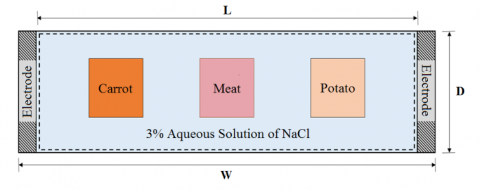
In the present study, four different cylindrical ohmic cells were numerically investigated using CFD (Computational Fluid Dynamics) techniques. The diameters of the cells studied are 16.5, 20.5, 24.5 and 28.5 mm. All the ohmic cells have 77 mm in total length (W), while the computational domain has only 76 mm in length (L); this difference is associated to the thickness of the electrodes, which is not considered in the computational domain. The computational domain adopted is axisymmetric and comprises four different foods: carrot, meat, potato and an aqueous sodium chloride solution. In order to represent the food particles, three 10 mm squares, with a distance of 10 mm between them, were used. Further details about the ohmic cell analyzed can be seen in Figure 1, where the dashed lines indicate the computational domain adopted:
Figure 1. Schematic representation of the ohmic cell studied
Similar to other studies carried out using the CFD techniques, in this work an extensive literature search was conducted in order to obtain the physical properties of the materials that make up the computational domain. Thus, values of density for all materials heated were taken from Pitzer and Peiper [11], Murakami [12] and Çengel and Ghajar [13]; values of thermal conductivity were obtained from Ozbek and Phillips [14], Slabani and Rahman [15] and mainly Çengel and Ghajar [13]; values of specific heat were gotten from Chen [16], Rao and Rizvi [17] and [13] again, while values of dynamic viscosity for the fluid medium were given by Kestin et al. [18]. Regarding the electric conductivity, the mathematical functions used by Shim et al. [19] to represent the behavior of this property with the temperature were adapted and used here as polynomial equations of 5th order, such procedure was adopted simply to facilitate the numerical implementation of the variation of this property with temperature. Therefore, only the electrical conductivity was modeled considering the variations caused by the temperature. Further details about the physical properties adopted are presented in the Table 1.
Table 1. Physical properties of the materials/food modeled
|
Carrot |
Values |
|
|
Density (kg.m-3) Specific Heat (kJ.kg-1.K-1) Thermal Conductivity (W.m-1.K-1) Electrical Conductivity (S.m-1) |
1029 3.90 0.570 3.247389x10‑9T5 – 5.560101x10‑6T4 + 3.796416x10‑3T3 – 1.292028T2 + 219.1637T - 1.48239x10⁴ |
|
|
Meat |
Values |
|
|
Density (kg.m-3) Specific Heat (kJ.kg-1.K-1) Thermal Conductivity (W.m-1.K-1) Electrical Conductivity (S.m-1) |
1090 3.54 0.498 0.031T – 6.7701a |
|
|
Potato |
Values |
|
|
Density (kg.m-3) Specific Heat (kJ.kg-1.K-1) Thermal Conductivity (W.m-1.K-1) Electrical Conductivity (S.m-1) |
1055 3.64 0.471 9.4082x10⁻⁹T5 – 1.596173x10‑5T4 + 1.080201x10⁻²T3 – 3.644712T2 + 613.1243T - 4.113914x10⁴ |
|
|
Aqueous Solution of NaCl |
Values |
|
|
Density (kg.m-3) Specific Heat (kJ.kg-1.K-1) Thermal Conductivity (W.m-1.K-1) Dynamic Viscosity (µ.Pa.s) Electrical Conductivity (S.m-1) |
1021 4.02 0.600 1043.2 0.1018T – 24.977b |
|
a Valid only when 293 K < T < 370 K
b Valid only when 290 K < T < 380 K
2.2 Mathematical and numerical model
The governing equations of the problem investigated are the conservative equations of continuity, energy and momentum, Eqns. (1), (2) and (3), respectively [20]:
$\frac{\partial \rho }{\partial t}+\nabla .(\rho \vec{U})=0$ (1)
$\frac{\partial (\rho h)}{\partial t}+\nabla .(\rho \vec{U}h)=\nabla .(k\nabla T)+\vec{S}$ (2)
$\frac{\partial (\rho \vec{U})}{\partial t}+\nabla .(\rho \vec{U}\vec{U})=-\nabla p+\nabla (\mu \nabla \vec{U})+pg+\vec{F}$ (3)
where ρ is the density (kg.m-3), t is the time (s), ∇ is the nabla operator, $\vec{U}$ is the velocity vector (m.s-1), h is the specific enthalpy (J.kg-1), k is the thermal conductivity (W.m-1.K-1), T is the temperature (K), S is the energy source term (W.m-3), p is the pressure (Pa), µ is the dynamic viscosity (Pa.s), g is gravity acceleration (m.s-2) and $\vec{F}$ is the momentum source term (N.m-3).
The hypotheses suggested by Zhang and Fryer [21], where the velocity field is not considered and the heat transfer by conduction is the main thermal mechanism, are adopted here. With these hypotheses, both regions (particles and liquid) of the computational domain can be treated as solid. Therefore, the convective term in Eq. (2) can be omitted, so that the Eq. (2) takes the following form [21]:
$\frac{\partial (\rho h)}{\partial t}=+\nabla .(k\nabla T)+\vec{S}$ (4)
According to Shim et al. [19], the energy source term (S) is the responsible for the conversion of the electrical energy into heat. In a conductive material, this source is given by a simple equation involving the electrical conductivity of the medium and the voltage applied. Thus, using the User Defined Functions (UDFs), the energy source term (S) implemented in the ANSYS FLUENT has the following form:
$\vec{S}={{\sigma }_{(T)}}{{\left| \nabla V \right|}^{2}}$ (5)
where σ is the electrical conductivity (S.m-1) as a function of temperature and V is the voltage (V).
Regarding the electrical field distribution, the Laplace’s equation presented by De Alwis and Fryer [8] provides this variable at any location of the ohmic cell. In other words, the electrical field distribution at any point of the computational domain is obtained solving the Eq. (6).
$\nabla (\sigma .\nabla V)=0$ (6)
2.3 Initial and boundary conditions
In a numerical simulation performed by CFD, initial and boundary conditions are necessary to solve the governing equations of the problem studied. The correct choice of these conditions is a critical step in the numerical studies, once the physical consistency of the results obtained is dependent of the adopted conditions. In the present work, only one initial condition was adopted (temperature when t = 0), while two types of boundary conditions were used to solve the governing equations: electrical boundary conditions and thermal boundary conditions.
2.3.1 Initial condition
$T(\forall x,\forall y,t=0)={{T}_{0}}$ (7)
where To is equal to 293 K.
2.3.2 Electrical boundary conditions
$V(x=0, \forall y, \forall t)=0 \mathrm{V}\\ [valid for the left electrode]$ (8)
$V(x=0,\forall y,\forall t)=20,\text{ 30, 40 or 50 V}\\ [valid for the right electrode]$ (9)
$\nabla V(\forall x, \forall y, \forall t) \cdot\left.\vec{n}\right|_{\text { wall }}=0\\ [valid for the particles surfaces]$ (10)
where $\vec{n}$ is the normal vector.
2.3.3 Thermal boundary conditions
$k \nabla T(\forall x, \forall y, \forall t) \cdot\left.\vec{n}\right|_{\text { wall }}=0\\ [valid for the electrodes and walls of the ohmic cell]$ (11)
2.4 Simulation parameters
In the present study, the Finite Volume Method is employed to solve the governing equations. All numerical simulations necessary to achieve the objectives proposed were carried out using the commercial software ANSYS FLUENT 16.1. In this software, a rectangular grid was used to represent the computational domain modeled. The most appropriate grid was chosen after a grid independence test, where three grids with different number of elements were tested for each ohmic cell analyzed, totaling 12 grids tested. All grids tested are rectangular, two-dimensional and refined near the food particles. The results of the test performed did not show significant differences between the grids tested. Therefore, in order to reduce the computational workload, the grids less refined were used in all simulations performed. Thus, the results presented here were obtained using four different computational grids: a computational grid with 7.000 elements used to represent the smallest ohmic cell (diameter of 16.5 mm); a computational grid with 8.100 elements used to represent the ohmic cell with diameter of 20.5 mm; a computational grid with 10.200 elements used to represent the ohmic cell with diameter of 24.5 mm and a computational grid with 11.580 elements used to represent the biggest ohmic cell (diameter of 28.5 mm). Figure 2 shows the computational grid used in the ohmic cell with 24.5 mm in diameter.
Figure 2. Grid used to represent numerically the ohmic cell with diameter of 24.5mm
Regarding the time step, a value of 0.01 s with a maximum of 1000 iterations per time step was used here. This value was chosen after a careful examination of the preliminary results obtained with other values (0.001, 0.002 and 0.005 s). Although the adopted value is relatively higher than the others, the results obtained using this value did not differ strongly from the other results. Thus, the value adopted (0.01s) proved to be most appropriate for this study, since through its use a considerable reduction in the total time of simulation is reached without compromising the results quality. Another important factor that interferes directly in the quality of the results obtained, as well as in the total processing time, is the convergence criteria adopted. In the present work, different convergence criteria were prescribed for the governing equations; a convergence criterion of 10-8 was used for the energy equation and a criterion of 10-5 was adopted for the continuity and velocity components equations (which are solved by the software even with the hypothesis of null velocity field).
2.5 Model validation
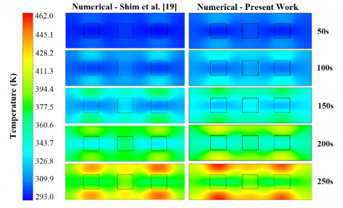
In order to verify whether the mathematical and numerical model implemented is appropriate for the study carried out, the study performed by Shim et al. [19] was reproduced for validation purposes. The problem studied by Shim et al. [19] is very similar to the investigated in the present study using the ohmic cell with diameter of 24.5 mm. The numerical validation was performed by means two different approaches: one qualitative and other quantitative. While the qualitative validation comprises a simple visual comparison of the temperature fields obtained in both numerical studies (Shim et al. [19] and the present study), the quantitative validation involves the comparison between the temperature obtained numerically in the geometrical center of each food and the values found experimentally by Shim et al. [19].
Figure 3 presents the temperature fields obtained by Shim et al. [19] and the temperature fields obtained in the present work. As can be seen, the results are very similar, with a pronounced heating region around the particles, especially above and below of them. This behavior is also observed by De Alwis and Fryer [8], which simulated two different problems: a generic food particle immersed in a liquid with a higher electrical conductivity (i) and a liquid with a lesser electrical conductivity (ii). In the problems where the electrical conductivity of the particles was lower than those of liquids, De Alwis and Fryer [8] reported the appearance of hot spots adjacent to the top and bottom of the particles, which is related to the high electric current density in these regions. As the liquid medium is more conductive than the particles, a smaller resistance to electron passage may be associated to the liquid regions, so that a higher current density is produced and a more pronounced heating is generated in the regions located around the particles. Therefore, the temperature distribution obtained in the present work is consistent with the theoretical background and other results available in the literature.
Figure 3. Temperature fields of the ohmic cell studied by Shim et al. [19] and the present work
Results of the quantitative validation is illustrated on the side (Figure 4), where the graph A shows the temperature in the geometric center of the carrot particle, the graph B the temperature in the meat particle and the graph C the temperature in the potato particle. As can be seen, there are a great similarity between both numerical results. Moreover, the results obtained in the present work show good agreement with the experimental results presented by Shim et al. [19], especially in the first 200 seconds. After this instant, in the meat particle, a considerable divergence between the numerical results and the experimental results is detected. The divergence observed only for this particle may be associated with a main reason: the difficulty faced by Shim et al. [19] in maintain the thermocouple correctly positioned in the meat particle. According to the authors, the meat tissues lost firmness during the heating, which done it impossible to position correctly the thermocouple in the meat particle, consequently, errors of unknown magnitude are associated with the experimental results of the meat particle. Although identified the main reason for the divergence observed, it should be noted that other empirical factors may also affect the experimental and numerical analyzes of ohmic heating process applied to meat particles. According to Zell et al. [22], the orientation of the muscle fibers, for example, plays a fundamental role in the ohmic heating process, since this factor affects the electrical conductivity of the meat and its heating. Thus, considering the results obtained here for the particles studied (carrot, meat and potato), as well as all the difficulties related in the literature in promoting a study about the ohmic heating of a meat particle, it can be stated that the mathematical and numerical model implemented is suitable for the numerical study of the ohmic heating process applied to food particles.
Figure 4. Temperature vs. time for experimental and numerical results of Shim et al. [19] and present work
After validated the model implemented, the numerical simulations used to analyze the effect of voltage in the heating process were conducted using the cell diameter of 24.5 mm. Temperature measurements, at different instants, were performed in the geometric center of the food particles, which were heated to a temperature limit (370 K). Since there is no information about the physical properties of the food particles after this temperature, this limit had to be considered. The results obtained for different voltages are shown in the Figure 5 (a-c), which presents the temperature plotted over the time for the carrot particle [Figure 5 (a)], meat particle [Figure 5(b)] and potato particle [Figure 5 (c)].
Figure 5. Temperature vs. time considering the voltage, for: (a) carrot, (b) meat and (c) potato particle
As can be seen, the use of higher values of voltage provided higher heating rates. Comparing the temperature profile in the carrot particle [Figure 5 (a)], it can be seen that to reach about 335 K it is needed 2 min of heating using 50 V and 9 min (a time 450% greater) using 20 V. Thus, the most intense heating was obtained with the highest voltage tested (50 V). Although high heating rates were obtained with the highest value of voltage tested (50V), it should be noted that this voltage is inappropriate for industrial processing purposes. As high production yields are targeted by the food industrial sector, even higher voltage values are required so that a solid-liquid mixture can be quickly sterilized, which does not occur when a voltage of 50 V is used. Similar results regarding the effect of the voltage in the ohmic heating process can be found in the literature, as in the studies conducted by Piette et al. [23] (cooking of meat sausages by OH) and Sarkis et al. [24] (heating of blueberry pulp by OH). Although both studies did not aim to analyze the effect of voltage under the heating rates generated, an attentive analysis of the results presented allows to verify that the highest heating were obtained when the highest voltage were adopted, exactly the same behavior observed here. Therefore, the voltage applied plays a key role in the ohmic heating process.
In order to analyze the uniformity of the OH, the temperature profiles obtained in the different food particles, for a fixed voltage, are presented in Figure 6 (a-b).
Figure 6. Temperature profiles in the different food particles for: (a) 20 V and (b) 50 V
For 20 V [Figure 6 (a)] it can be seen a very homogenous heating, with tiny differences in the temperatures. However, using 50 V [Figure 6 (b)], the temperature profiles are similar, but it can be seen a difference in the meat particle temperature which is related to its higher electrical conductivity when compared to the other particles (at 330 K, the electrical conductivity of meat, potato and carrot are 3.46, 0.55 and 0.45 S.m-1, respectively). As the electrical conductivity is an increasing function of temperature, a more pronounced heating affects more intensively its variation, especially when the function that governs its growth has a more intense character, like the meat particle. Since the higher voltage applied (50V) provided a more intense heating, the electrical conductivity of the particles varied with greater intensity in this case, which caused the meat particle to present values of electrical conductivity substantially higher than those associated with the other foods. In addition to the applied voltage, higher values of electrical conductivity also allow the generation of higher heating rates, as reported in the literature [8-10]. Thus, due to it is the most conductive particle in the medium, the meat particle underwent a more intense heating than the other particles, which gave rise to an undesirable temperature gradient in the solid-liquid mixture.
Two different numerical simulations are conducted to investigate the role of the ohmic cell diameter (D) in the heating process. In the first study, the electrode has the same size of the ohmic cell diameter, as presented in the shaded areas of the Figure 1. Four different diameter values are used (16.5, 20.5, 24.5 and 28.5 mm) in the simulations, being the voltage applied fixed in 50 V. Since the temperature profiles were not strongly influenced by the diameters, only the two extremes diameters are chosen to be plotted in Figure 7 (a-c).
Figure 7. Temperature profiles in the different food particles for the smallest (16.5 mm) and the biggest (28.5 mm) diameters tested, for: (a) carrot, (b) meat and (c) potato
While Figure 7 (a) presents the temperature profiles for diameters of 16.5 and 28.5 mm for the carrot particle, Figure 7(b) presents the temperature profiles for meat particle and Figure 7 (c) for the potato particle. As can be observed, the profiles of the meat particle are practically the same, with a slightly higher heating in the larger diameter problem (28.5 mm). Tiny differences are observed for carrot and potato, which increase as time increases. Unlike to meat particle, these foods (carrot and potato) obtained a more pronounced heating with the smallest diameter tested; which indicates that the heating rate obtained may be associated to several factors besides the ohmic cell diameter. Thereby, it is possible to conclude that the heating generated was not influenced only by the ohmic cell diameter, but by multiple factors.
In the second study, the ohmic cell diameter was maintained fixed in 24.5 mm, while two different sizes of the electrodes were tested: 10 and 24.5 mm. Figure 8 (a-c) shows the temperature profiles of the different food particles, using different electrodes sizes. As observed, the profiles are similar with differences which increase as time passes. The highest difference occurs for the meat particle (11.94 K at 138 s). Thus, based on these results, it can be stated that the heating generated was influenced by the electrode size, where the larger electrodes provided the higher heating rates.
Figure 8. Temperature profiles for the two electrodes size
Although it is a factor of possible relevance for the OH technology, little is known about the importance of the spatial position of the particles regarding the generated heating. In this way, assuming the same spatial arrangement of Figure 1 for two different diameters (16.5 and 28.5 mm), the role of the particles position was investigated using simulations where all the particles were composed of a single food.
The results obtained are shown in Figure 9 (a-c), where [Figure 9 (a)] presents the temperature profile of the carrot particles, [Figure 9 (b)] the meat particles and [Figure 9 (c)] the potato particles.
Figure 9. Temperature profiles for the problems where all the particles were composed of the same food, as: (a) carrot, (b) meat and (c) potato
As can been seen, the lowest temperatures are associated with the central particle of all the cases studied, especially when the largest diameter is adopted, which is consistent with the behavior observed in Figure 7 (b). While the largest temperature difference observed for the problems involving the smallest diameter tested (16.5 mm) was 1.1 K at 138s (between particles 1 and 2 of carrot), the highest difference associated with the problems involving the biggest diameter used (28.5 mm) was 3.9 K at 138s (between particles 1 and 2 of meat). In other words, the ohmic cell diameter and the spatial positioning of the particles may influence the temperature distribution inside the equipment, but not significantly using this value of voltage (50V).
In the present work, some aspects related to the ohmic heating (OH) technology were investigated using the ANSYS Fluent 16.1. The computational domain adopted is axisymmetric and represents a cylindrical ohmic cell used to heat pieces of carrot, meat and potato within an aqueous NaCl solution. From this geometry, the following conclusions can be drawn:
The authors acknowledge the financial support of CAPES – Coordenação de Aperfeiçoamento de Pessoal de Nível Superior (Coordination for the Improvement of Higher Education Personnel) and UNISINOS – Universidade do Vale do Rio dos Sinos (University of Vale do Rio dos Sinos).
|
D F g h k L p S T t U V W |
ohmic cell diameter, m momentum source term, N.m-3 gravitational acceleration, m.s-2 specific enthalpy, J. kg-1 thermal conductivity, W.m-1. K-1 computational domain lenght, m pressure, Pa energy source term, W.m-3 temperature, K time, s velocity, m. s-1 voltage, V ohmic cell total lenght, m |
|||
|
Greek symbols
|
|
|
||
|
r s |
density, kg. m-3 electrical conductivity, S.m-1 |
|
||
|
µ |
dynamic viscosity, kg. m-1.s-1 |
|
||
[1] Mercali, G., Jaeschke, D., Tessaro, I., Marczak, L. (2012). Study of vitamin C degradation in acerola pulp during ohmic and conventional hear treatment. LTW – Food Science and Technology, 47(1): 91-95. http://dx.doi.org/10.1016/j.lwt.2011.12.030
[2] Ruan, R., Ye, X., Chen, P., Doona, C., Taub, I. (2001). Ohmic heating. In: Richardson, P.S. (eds), Thermal Technologies in Food Processing. Woodhead Publishing Limited, Londres.
[3] Fryer, P. (1995). Electrical resistance heating of foods. In: Gould, G.W. (eds) New Methods of Food Preservation. Blackie Academic & Professional, Glasgow.
[4] Sakr, M., Liu, S. (2014). A comprehensive review on applications of ohmic heating (OH). Renewable and Sustainable Energy Reviews, 39: 262-269. https://doi.org/10.1016/j.rser.2014.07.061
[5] Abdulmunem, A., Jalil, J. (2018). Indoor investigation and numerical analysis of PV cells temperature regulation using coupled PCM/fins. International Journal of Heat and Technology, 36(4): 1212-1222. https://doi.org/10.18280/ijht.360408
[6] Benlekkam, M., Nehari, D., Madani, H. (2018). The thermal impact of the fin tilt angle and its orientation on performance of PV cell using PCM. International Journal of Heat and Technology, 36(3): 919-926. https://doi.org/10.18280/ijht.360319
[7] Buonomo, B., Pasqua, A., Ercole, D., Manca, O. (2018). Entropy generation analysis of parallel plate channels for latent heat thermal energy storages. TECNICA ITALIANA – Italian Journal of Engineering Science, 61(1): 42-48. https://doi.org/10.18280/ti-ijes.620106
[8] De Alwis, P., Fryer, P. (1990). A finite-element analysis of heat generation and transfer during ohmic heating of food. Chemical Engineering Science, 45(6): 1547-1559. http://dx.doi.org/10.1016/0009-2509(90)80006-z
[9] Sastry, S.K., Palaniappan, S. (1992). Mathematical modeling and experimental studies on ohmic heating of liquid-particle mixtures in a static heater. Journal of Food Process Engineering, 15(4): 241-261. http://dx.doi.org/10.1111/j.1745-4530.1992.tb00155.x
[10] Salengke, S., Sastry, S.K. (2007). Experimental investigation of ohmic heating of solid-liquid mixtures under worst-case heating scenarios. Journal of Food Engineering, 83(3): 324-336. http://dx.doi.org/10.1016/j.jfoodeng.2007.02.060
[11] Pitzer, K., Peiper, J. (1984). Thermodynamic properties of aqueous sodium chloride solutions. Journal of Physical and Chemical Reference Data, 13(1): 1-102. http://dx.doi.org/10.1063/1.555709
[12] Murakami, E. (1997). The thermal properties of potatoes and carrots as affected by thermal processing. Journal of Food Process Engineering, 20(5): 415-432. http://dx.doi.org/10.1111/j.1745-4530.1997.tb00431.x
[13] Çengel, Y., Ghajar, A. (2009). Heat and Mass Transfer: Fundamentals and Applications. McGraw-Hill.
[14] Ozbek, H., Phillips, S. (1980). Thermal conductivity of aqueous sodium chloride solutions from 20 to 330 °C. Journal of Chemical and Engineering Data, 25(3): 263-267. http://dx.doi.org/10.1021/je60086a001
[15] Sablani, S., Rahman, M. (2003). Using neural networks to predict thermal conductivity of food as a function of moisture content, temperature and apparent porosity. Food Research International, 36(6): 617-623. http://dx.doi.org/10.1016/s0963-9969(03)00012-7
[16] Chen, C. (1982). Specific heat capacities of aqueous sodium chloride solutions at high pressures. Journal of Chemical and Engineering Data, 27(3): 356-358. http://dx.doi.org/10.1021/je00029a038
[17] Rao, M., Rizvi, S. (1994). Engineering Properties of Food. Marcel Dekker.
[18] Kestin, J., Khalifa, H., Correia, R. (1981). Tables of the dynamic and kinematic viscosity of aqueous NaCl solutions in the temperature range 20-150 °C and the pressure range 0.1-35 Mpa. Journal of Physical and Chemical Reference Data, 10(1): 71-88. http://dx.doi.org/10.1063/1.555641
[19] Shim, J., Lee, S., Jun, S. (2010). Modeling of ohmic heating patterns of multiphase food products using computational fluid dynamics codes. Journal of Food Engineering, 99(2): 136-141. http://dx.doi.org/10.1016/j.jfoodeng.2010.02.009
[20] Ansys Fluent Theory Guide 14.0. (2013). Ansys Inc., Canonsburg, USA.
[21] Zhang, L., Fryer, P. (1993). Models for the electrical heating of solid-liquid food mixtures. Chemical Engineering Science, 48(4): 633-642. http://dx.doi.org/10.1016/0009-2509(93)80132-a
[22] Zell, M., Lyng, J., Cronin, D., Morgan, D. (2009). Ohmic heating of meats: electrical conductivities of whole meat and processed meat ingredients. Meat Science, 83(3): 563-570. https://doi.org/10.1016/j.meatsci.2009.07.005
[23] Piette, G., Buteau, M., Halleux, D., Chiu, L., Raymond, Y., Ramaswamy, H., Dostie, M. (2004). Ohmic cooking of processed meats and its effects on product quality. Journal of Food Science, 69(2): 71-78. https://doi.org/10.1111/j.1365-2621.2004.tb15512.x
[24] Sarkis, J., Jaeschke, D., Tessaro, I., Marczak, L. (2013). Effects of ohmic and conventional heating on anthocyanun degradation during the processing of blueberry pulp. LWT – Food Science and Technology, 51(1): 79-85. http://dx.doi.org/10.1016/j.lwt.2012.10.024