Yashraj Patil![]() | Harikrishnan Ramachandran*
| Harikrishnan Ramachandran*![]() | Harshita Gupta
| Harshita Gupta![]() | Naresh Ganeshi
| Naresh Ganeshi![]() | Dorian Janney
| Dorian Janney![]()
© 2024 The authors. This article is published by IIETA and is licensed under the CC BY 4.0 license (http://creativecommons.org/licenses/by/4.0/).
OPEN ACCESS
In the context of climate change, the present study analysed significant shifts in climatic trends on the dataset available from 1981 to 2022 of the Koyna wildlife sanctuary, a UNESCO biodiversity hotspot. The analysis adopts correlation and heatmap methods, utilizing the Pearson coefficient for trend analysis of rainfall, temperature, relative humidity, and surface pressure, a key climatic variable affecting ecosystem climates. The selection of these methods allows handling multivariate analyses for a subtle understanding of the interplay between these variables over time. Findings revealed increasing trends in rainfall and temperature, consistent surface pressure patterns, and stable relative humidity. Notably, Relative Humidity displayed significant associations with rainfall, surface pressure, and maximum temperature, suggesting collective influences on its fluctuations. The pivotal year, 2019, marked increased weather dynamics, aligning with the positive phase of the Indian Ocean Dipole. The prolonged Indian summer monsoon since 2019, disrupting the October heat transition, poses challenges for ecosystems, and soil conditions. The observed climatic trends, particularly the increased rainfall and temperature, underscore the urgent need for adaptive biodiversity conservation and management strategies within the sanctuary possibly enhancing habitat connectivity to allow for species migration and rescue measures to combat the effects of prolonged wet & dry periods. These findings call for the sanctuary's management to incorporate climate trend insights into their conservation tactics, ensuring the sanctuary's diverse ecosystems and species are resilient in the face of evolving climate conditions.
biodiversity hotspot, climate change study, climatic trend analysis, experiential validation, October heat
The climate is a vital part of the Earth's system, and its significance for nurturing forest ecosystems cannot be undervalued. We are observing shifts in the patterns of the climatic cycle, leading to increased intensity that consistently surpasses the average threshold values of different climatic variables with every passing year, it is essential to study how the climate is influencing the forest ecosystem and identify the trends and major shifts observed during a specific period of time. “Climate-change impacts have led to visible shifts on the terrestrial systems in many parts of Asia in the phenologies, growth rates and distributions of plant species” (IPCC COP 27, Chapter 10-Asia) [1]. Extirpation risks in percentages of taxa (plants, amphibians, reptiles, birds, and mammals) for 2℃ and 4.5℃ global warming in Asia's 'priority places' without adaptation by the 2080s show 18.8% extirpation at 2℃ and 41.67% extirpation at 4.5℃ in the Indian Western Ghats Biodiversity Hotspots (IPCC COP 27, Chapter 10-Asia) [1].
The study performed by Vose et al. [2] stated that climate directly affects forests by impacting their makeup, behaviour, and well-being. Alterations in weather like rain and temperature can directly influence forests, but the outcomes vary based on location and the type of forest. Certain outcomes can be positive, while others might be negative. For instance, warmer conditions could boost tree growth in specific forests but reduce it in different ones. In many studies, the temperature and precipitation relationships are referred in any climate studies while other parameters like relative humidity and surface pressure (atmospheric pressure) are often kept aside though all these four have a crucial interplay in driving the climate of a particular region.
The climatic trend analysis study is carried out on the data of Koyna Wildlife Sanctuary (WLS) which is in Satara District of Maharashtra State. Nandargi and Mulye [3] studied the interplay between Intensity of Indian Summer Monsoon Rainfall at the Koyna during the period from 1961 to 2005. While Jha et al. [4] studied the geothermal gradient of boreholes to estimate the past variations in the climate. Bajirao et al. [5] used remote sensing and geographical information system technology to conduct an area-altitude analysis of erosional topography investigation of Koyna River basin. While the Koyna region has seen various research studies in the fields of seismology, Dam structure, and geology, the focus on Climatic Studies remains relatively limited. Aside from the seasonal rainfall analysis conducted by Nandargi and Mulye [3], there is a notable gap in research concerning the region's climatic factors and their impact on the forest ecosystem. Therefore, it is imperative to gain a comprehensive understanding of the trends in climatic variables and their influence on the region's forest ecosystem. The study by Patil et al. [6] state that on August 5th, 2019, the regions of Sangli and Karad (Satara District) experienced heavy rainfall and a sudden surge in water discharge from the Koyna Dam, surpassing 50,000 cusecs. Similarly, the Chandoli Dam released approximately 20,000 cusecs of water, causing disruption in communication between numerous villages in Sangli and Kolhapur District. These unprecedented events led to the first-ever devastating floods in the history of western Maharashtra. The floodwaters submerged vast areas in the vicinity of the river and its tributaries, severely impacting the three districts and causing significant devastation. Table 1 summarizes the recent studies done on the Koyna WLS with respect to climate study.
Table 1. Research studies done in Koyna WLS with respect to climatic parameters research
|
Author & Year |
Methodology |
Result |
|
Nandargi and Mulye [3] |
Analysed daily rainfall data, formed normalized rainfall curves. Used tangent slopes and correlation analysis for distribution patterns and rain intensity. |
Diverse monsoon means daily rainfall. Heavy rain days (10-15%) contribute significantly. Intense rainfall days (33% of rain days) notable in Koyna catchment. |
|
Jothiprakash and Fathima [7] |
Utilized correlation dimension method to analyze irregular behaviour of daily average rainfall data from Koyna reservoir catchment. |
Revealed chaotic behaviour in average rainfall of Koyna region using correlation dimension method. Effects of radius, scaling region, and time steps varied in behaviour assessment. |
|
Jha et al. [4] |
Used borehole geothermal gradient in Koyna to calculate a century-long warming. Validated with surface air temperature profiles. |
Found a considerable century-long warming trend in Koyna. Validation with surface air temperature profiles confirmed this warming trend. |
|
Bajirao et al. [5] |
Employed Remote Sensing (RS) and Geographical Information System (GIS) technology. Conducted Area-altitude analysis of erosional topography in Koyna river basin. |
Remote sensing and GIS technology used for an Area-altitude analysis of erosional topography investigation in Koyna river basin. |
Table 2. Research gap with respect to parameters considered in previous studies
|
Parameter |
Previous Study |
Research Gap |
|
Temperature |
Often considered in climate studies, partially addressed. |
Limited focus to its interaction with other parameters |
|
Rainfall |
Frequently studied, acknowledged relationship. |
Incomplete integration with other influencing factors. |
|
Relative Humidity |
Often overlooked, not extensively explored. |
Neglected despite its role in climate dynamics. |
|
Surface Pressure |
Often neglected, underrepresented. |
Lack of study of its role in the region. |
|
Climatic Trend Study |
Limited focus on Koyna biodiversity hotspot region's climatic trends concerning rainfall only. |
Gap in investigating the long-term trend of climate variables considering all atmospheric parameters. |
What is Indian Ocean Dipole (IOD)?
The Indian Ocean Dipole (IOD) is a climate phenomenon characterized by changes in sea surface temperatures in the Indian Ocean. It is similar to El Nino and La Nina events, but it is specific to the Indian Ocean region. The Indian Ocean Dipole (IOD) has two phases: a positive phase with warmer seas in the west and cooler waters in the east, and a negative phase with the opposite pattern. These sea surface temperature anomalies can have significant effects on weather patterns, influencing things like rainfall and temperature in the surrounding areas [8-10].
Furthermore, the Indian Summer Monsoon (ISM) exhibited remarkable behaviour, being abnormally dry in June but becoming impressively wet by September. The positive IOD event, which was characterized by sea surface temperature anomalies in the Indian Ocean, had a substantial impact on weather patterns in the region.
The research gap with respect to study performed till date in Koyna WLS can be seen in Table 2 and parameters that are considered most and least in the studies till date.
According to “Expert Study Committee Report: FLOODS 2019 (KRISHNA BASIN) by Water Resource Department, Government of Maharashtra, India” [8], the region experienced persistent and intense rainfall activity, coinciding with an active monsoon spell that commenced on July 27, 2019, affecting Maharashtra. This resulted in significant floods in Konkan and North Madhya Maharashtra. Following that, on August 3, 2019, another vigorous monsoon spell began, drove by the emergence of a low-pressure system over the Northeast Bay of Bengal. In the next days, the system deepened into a deep depression and travelled westward, causing catastrophic flooding in South Madhya Maharashtra. The deep depression system moved across central India, characterized by an active low-pressure system with wind gusts. This movement had a significant impact on Madhya Maharashtra's west coast and ghat areas, resulting in increased rainfall. These areas saw heavy to very heavy rainfall and even extremely heavy rainfall events over the period of more than a week, culminating in serious flooding. The prolonged and heavy rain during this timeframe exacerbated flood conditions and provided considerable problems to the impacted areas.
Ratna et al. [9] performed a study to better comprehend the underlying causes that contributed to the abrupt increase in heavy downpours in 2019. The study's findings confirmed the presence of a positive Indian Ocean Dipole (IOD) event in the year 2019, which was one of the strongest in the recorded history.
The Koyna Wildlife Sanctuary (WLS), recognized for its rich forest vegetation comprising Southern Tropical Evergreen Forest and Southern Moist Mixed Deciduous Forest [11], stands as a vital ecological and hydrological asset. In 2012, UNESCO designated it as a World Heritage Site, acknowledging its global significance for biodiversity conservation. Additionally, the Government of India had earlier, in 1985, declared it a protected area, underscoring its environmental importance. The sanctuary holds the status of an IUCN Category 4 Site [12], emphasizing habitat and species management for conservation. Central to the sanctuary's ecological significance is the Koyna Dam on the Koyna River, a major tributary of the Krishna River. This dam not only serves hydrological purposes but also houses a hydroelectric power plant with a 1920 megawatts capacity, marking the intersection of environmental conservation and energy generation. Despite its recognized importance in various domains, including hydrology and seismology, there remains a gap in comprehensive climatic studies within this region. This oversight highlights the urgent need for detailed climatic trend analysis to understand and mitigate the impacts of climate change on this critical biodiversity hotspot, making the present study both timely and essential.
The reasons that justify this research are: 1) The study region lacks substantial investigations concerning climatic variables with a focus on temporal variability, a primary aspect addressed in this study. 2) The chosen study period of 41 years is suitable for climate change assessment and to understand the trend of variables. Throughout this research, the study intends to answer the following questions: 1) How did the variables that are selected in the research area shows a trend from 1981 to 2022? 2) When was the significant shift in climatic intensification seen during a 41-year period, and how constant has it been since then? 3) Is there an impact of Indian Ocean Dipole (IOD) Effect on any identified climatic intensification?
In this research, the Rainfall (mm/day), Temperature (Max, Mean, Min), Relative Humidity (%) and Surface Pressure (hPa) variables are considered, and data is taken between the year 1981 to 2022 to understand the climate change trend in climate over the region. In this study, daily data for a single year is collected for each variable, and a correlation analysis using Pearson's coefficient (r) is conducted, visualized through heatmaps. This analysis aimed to explore the relationships and interplay between these factors, shedding light on their potential influences on weather patterns and conditions. To understand the overall trend of the correlation (r) values, a line plot was generated, encompassing data from 41 years for each variable pair. Interestingly, the year 2019 stood out as a pivotal point, exhibiting a significant shift in climate patterns, notably with the highest recorded values for Temperature (max, mean, min), and Rainfall. After this shift, both variables have displayed a consistent growth pattern. These findings underscore the importance of investigating the impact of climatic changes on the studied variables over the past four decades.
2.1 Study area
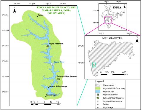
The Koyna Wildlife Sanctuary (WLS) located in Satara District of Maharashtra State in the Western Ghats covers an area of 423.55 square kilometers and possess an elevation between 600 meters to 1000 meters of altitude [13]. Figure 1 shows the map of Koyna WLS situated between latitudes 17.20° and 17.50° N and longitudes 73.30° and 73.55° E.
Figure 1. Biodiversity hotspot- Koyna wildlife sanctuary
2.2 Climatic data
This study utilized NOAA/PMEL TMAP, ERA5 Land daily reanalysis datasets [14] available at Copernicus Climate Change Service (C3S) of the European Centre for Medium-Range Weather Forecasts (ECMWF). While, for cross analysis, the rainfall dataset was obtained from data of Global Precipitation Measurement (GPM) mission’s GPM_3IMERGM v06 [15] to generate the inter annual time series using NASA Giovanni Tool [16]. Table 3 shows the details of dataset used for study.
Table 3. Specification of different dataset used for the study
|
Dataset |
Source |
Availability |
Temporal Resolution |
|
ERA5-Land [14] |
C3S | ECMWF |
1981-present |
Daily, Monthly, Annual |
|
GPM_3IMERGM v06 [15] |
NASA GPM |
2000-present |
Monthly, Annual |
2.3 Methodology utilised
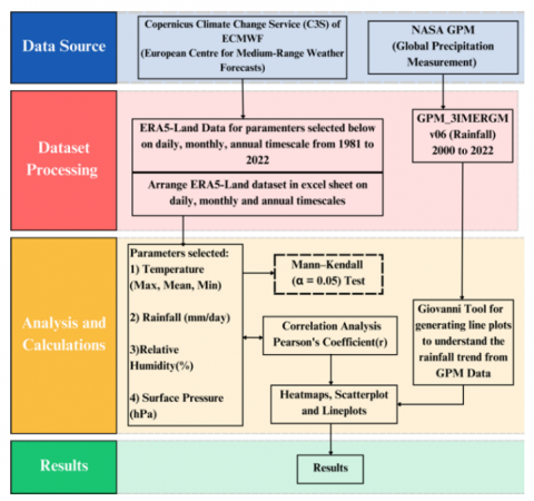
Figure 2 shows the flow of the methodology followed in this research. The study aims to analyze climatic variables within the Koyna Wildlife Sanctuary for the period from 1981 to 2022, with a focus on conducting trend analysis. To conduct the trend analysis, the variables namely temperature (maximum, minimum and mean) and rainfall data (in mm/day), relative humidity (%) and surface pressure (hPa) on daily timescale data are obtained from NOAA/PMEL TMAP ERA5-Land Data. All this data is then merged into a single Excel file, with the respective variables as column headings on daily timescale.
Figure 2. Graphical representation of flow of methodology
Why ERA5-Land and NASA GPM Data selected for climatic trend analysis study?
The ERA5-Land data provides a global coverage and consistency in the data over a long period. ERA5-Land is a reanalysis dataset which provides a consistent view of the evolution of land variables over several decades at an enhanced resolution compared to ERA5. Reanalysis produces the data that goes several decades back in time, providing an accurate description of the climate of the past.
The key advantage of ERA5-Land over ERA5 and the earlier ERA-Interim for any regional analysis is the horizontal resolution enhanced globally to 9 km compared to 31 km (ERA5) or 80 km (ERA-Interim), although the temporal resolution remains hourly as in ERA5. Horizontal resolution in a numerical weather or climate model refers to the size of the grid cells or grid spacing. Smaller grid cells with a lower horizontal resolution provide more detailed information but cover a smaller geographic area. A higher horizontal resolution, on the other hand, indicates larger grid cells that provide coarser or less detailed information but cover a broader geographic region.
When the ERA5-Land's horizontal resolution of 9 km is compared to ERA5's horizontal resolution of 31 km, it is seen that ERA5-Land has a lower (finer) resolution. ERA5-Land, on the other hand, gives more precise information for smaller geographic areas, making it better suited for localized and regional study. This improved detail can be useful for applications requiring great precision at local scales. Hence, to study a specific region’s climate dynamics, ERA5-Land dataset is best suitable with dataset of variables available as part of open-source initiative. Hence, ERA-5 Land dataset suits perfect to gain more detailed analysis of Koyna WLS.
In terms of NASA GPM Data, the multi-sensor approach of the GPM Satellite integrates data from multiple satellite sensors, including the Dual-frequency Precipitation Radar (DPR) and the Global Microwave Imager (GMI). This multi-sensor technique improves precipitation measurement accuracy and dependability, especially in places with complex terrain or several forms of precipitation. Because Koyna WLS is in the Indian Western Ghats and has complex terrain, as well as being a hydrological site, rainfall is a significant variable. However, there has been no rainfall-specific study using GPM data, so this study performs a 22-year analysis of precipitation based on the availability of GPM data since 2000.
Table 4 shows the ERA5-Land data collection and timescale and number of datapoints per climate variable namely, Temperature (Max), Temperature (Min), Temperature (Mean), Rainfall, Relative Humidity and Surface Pressure.
By utilizing statistical analysis, including Pearson's coefficient (r), a correlation matrix is established to examine the relationships between the obtained climatic data variables. Moreover, to comprehend the correlation (r) value and strength between different pairs of variables across all 41 years at a daily timescale, the ES1 generates a final heat map through correlation analysis. This comprehensive approach allows to gain valuable insights into how these climatic variables interact with one another and influence the climate in the Koyna Wildlife Sanctuary.
Table 4. Climate data organization for ERA5-land dataset for climate variables from 1981 to 2022
|
Data Timescale |
Excel Sheet |
Datapoints per Variable |
Total Datapoints for All 6 Variables Combined |
|
Daily |
Excel Sheet 1 (ES1) |
15,340 |
92,040 |
|
Monthly |
Excel Sheet 2 (ES2) |
504 |
3024 |
|
Annual |
Excel Sheet 3 (ES3) |
42 |
252 |
2.3.1 Methodological steps in detail
1. Data Source and Acquisition
2. Dataset Processing
3. Analysis and Calculations
2.3.2 Mann-Kendall’s test
The Mann-Kendall test [17-19] has proven to be a valuable tool for analysing trends in meteorological and climatic data. In this study, the Mann-Kendall test is applied to discover historical trends in relative humidity, rainfall, surface pressure and temperature data within the Koyna Wildlife Sanctuary (WLS) region in the Western Ghats of India, using a 41-year data spanning from 1981 to 2022 at daily timescale. The Statistic ‘Smk’ value of non-parametric Mann-Kendall test is calculated using Eq. (1), enabling the study to assess the presence and direction of trends in different climate variables patterns over the specified time from 1981 to 2022.
$S_{m k}=\sum_{p=1}^{n-1} \sum_{q=p+1}^n \operatorname{sgn}\left(X_q-X_p\right)$ (1)
where,
n is the number of datapoints in a sample;
Xq and Xp are from q=1,2,....,n-1, where q>1 and p=p+1,….,n;
And sgn (Xq-Xp) calculated using following Eq. (2):
$\operatorname{sgn}\left(X_q-X_p\right)\left\{\begin{array}{c}+1, \text { if }\left(X_q-X_p\right)>0 \\ 0, \text { if }\left(X_q-X_p\right)=0 \\ -1, \text { if }\left(X_q-X_p\right)<0\end{array}\right.$ (2)
To calculate test statistic Z, first there is need to obtain variance (S) using Eq. (3) as below:
$\begin{aligned} {var}(S)=\frac{1}{18}[\mathrm{n}( & \mathrm{n}-1)(2 \mathrm{n}+5) \left.-\sum_{\mathrm{p}=1}^{\mathrm{g}} \mathrm{t}_{\mathrm{p}}\left(\mathrm{t}_{\mathrm{p}}-1\right)\left(2 \mathrm{t}_{\mathrm{p}}+5\right)\right]\end{aligned}$ (3)
where,
n is number of datapoints,
g is the zero difference between compared values number, and tp is number of datapoints in pth group.
Now, the test statistic Z is calculated using Eq. (4):
$f(S)\left\{\begin{array}{l}\frac{S-1}{\sqrt{\operatorname{var}(S)}} \text { if } S>0 \\ 0, \quad \text { if } S=0 \\ \frac{S+1}{\sqrt{\operatorname{var}(S)}} \text { if } S<0\end{array}\right.$ (4)
From result, when Z > 0, the trend is an increasing trend, and when Z < 0, it’s a decreasing trend. When the confidence level a is introduced to check on statistical significance, the data would go through statistically significance trend if |Z|>Z (1-$\alpha$/2), where Z (1 - $\alpha$/2), where is the corresponding value of P=$\alpha$/2 that follows the standard normal distribution [20]. For this study, the 0.05 confidence level is considered.
To measure the magnitude of time series trend, a simple non-parametric method designed by Sen [21] is calculated by below the Eq. (5):
$\beta={Median}\left(\frac{x j-x i}{j-i}\right), j>i$ (5)
where, $\beta$ is Sen’s slope estimate, $\beta$ > 0 shows an upward trend in time series and vice versa.
2.3.3 Pearson’s coefficient
The Pearson coefficient (r) helps to understand how closely and in what direction two 227 things are linked in a linear relationship manner. It is like a measure of their connection 228 strength. It measures how closely the points on a graph for two parameters match up in a 229 straight line. The value of the Pearson coefficient ranges from ‘-1’ to ‘+1’, where ‘-1’ denotes 230 a perfect negative linear relationship, ‘0’ indicates no linear relationship, and ‘+1’ denotes a 231 perfect positive linear relationship [22]. To calculate the Pearson’s coefficient the following Eq. (6) is used:
$P_{(x, y)}=\frac{\sum_i x_i y_i-\left(\left(\sum_i x_i\right)\left(\sum_i y_i\right) / n\right)}{\sqrt{\left(\sum_i x_i^2-\left(\left(\sum_i x_i\right)^2 / n\right)\right)\left(\sum_i y_i^2-\left(\left(\sum_i y_i\right)^2 / n\right)\right)}}$ (6)
where ‘x’ and ‘y’ are variables and ‘n’ is the number of values and r = P(x,y).
Correlation analysis was performed on ERA-5 land daily timeframe data from 1981 to 2022. Each variable was correlated with every other variable during this study, resulting in the calculation of Pearson's coefficients (r-values) to measure the strength of association between these variables. These r-values for every pair of variables are calculated from daily data collected over a long period of time spanning 41 years, offering a thorough picture of the overall correlations between the variables.
In this analysis, it is recognized that Pearson's correlation coefficient provides a single overall measure of the relationship between two variables for the entire 41-year time series. To understand the changing nature of these relationships over time, The analysis involved calculating annual r-values for the relationship between two variables, spanning a 41-year period from 1981 to 2022. Starting with ERA5-Land daily timescale data spanning 41 years, calculate annual r-values for each year, resulting in 41 sets of r-values. Each row in the dataset represents one year, and the corresponding annual r-value reflects the strength of the relationship between two variables for that specific year. These 41 sets of r-values allow to observe how the association between the two variables evolved over time, identifying trends and fluctuations in the relationship's strength. By compiling these annual r-values for seven different variable combinations and visualizing them in a line plot, the analysis provides the insights into temporal variations in relationship strength. This approach complements the single r-value by offering a historical perspective, allowing to identify when relationships became weaker or stronger throughout the 41-year timeframe.
The combinations preferred are as below:
Then, all these values are used to generate a multi-line plot graph, which shows all relationship of variable in single plot with color codes for different line plots representing different relationship. For scatterplot generation, a pair of climate variables is selected to understand major atmospheric relationship.
Why are Scatterplot generated?
The scatterplot was generated with the primary objective of understanding the how one variable affects another variable selected for study. Additionally, it served as a tool to assess the accuracy of the dataset and determine whether it aligns with the predefined interplay of atmospheric variables dynamics. The results from the scatterplot have been highly encouraging as they precisely depict the expected relationship between the variables. This validation provides confidence in the dataset's reliability and consistency, and to proceed with further analyses and draw meaningful conclusions about the complex interactions within the climate system. The successful visualization of the expected interplay in the scatterplot validates the dataset's suitability for more in-depth investigations and enables to delve deeper into understanding the dynamics of the atmosphere and its impact on various climatic phenomena.
We used two different rainfall datasets, including ECMWF ERA5-Land and NASA GPM to find substantial variations in the climatic system of Koyna Wildlife Sanctuary (WLS). To visualize data trends and changes over time, line plots and trendlines were created. The NASA GPM Data Plot was generated with the Giovanni tool, and the ECMWF ERA5-Land data trend was generated with the Open Foris Earth Map Tool and Google Collab using annual timescale data.
The multifaceted outcomes of our investigation, which encompasses various climatic variables such as rainfall, temperature, relative humidity, and surface pressure. Followed by Mann-Kendall Test, the results further deepen to climatic trend analysis outcomes for both ERA5-Land and GPM Datasets.
3.1 Mann-Kendall test
The Mann-Kendall and Sen's slope test are two statistical techniques for trend analysis, particularly in time series data. They are frequently used to assess the presence of a monotonic trend over time in a of a variable in the dataset as well as its strength.
Table 5. Man-Kendall test result for ERA5-Land at annual timescale dataset from 1981 to 2022
|
Parameter |
Mann-Kendall Tau |
Mann-Kendall P-Value |
Sen’s Slope |
Statistical Significance |
|
Relative Humidity |
0.174317 |
1.04E-01 |
0.03625 |
No |
|
Rainfall |
0.261324 |
1.48E-02 |
13.247222 |
Yes |
|
Surface Pressure |
- 0.092969 |
3.86E-01 |
-0.004667 |
No |
|
Temp (Max) |
0.530542 |
7.70E-07 |
0.027692 |
Yes |
|
Temp (Min) |
0.449099 |
2.86E-05 |
0.03 |
Yes |
|
Temp (Mean) |
0.635996 |
3.24E-09 |
0.02359 |
Yes |
The Mann-Kendall test results as seen in Table 5 for the rainfall, temperature (max, mean, min) data show a statistically significant trend at the 5% level. The p-value of these variables are almost 0.002 is less than the chosen significance level of 0.05, providing strong evidence against the null hypothesis and supporting the presence of a meaningful trend in the data. The surface pressure and relative humidity data Mann-Kendall test results show that the trend is not statistically significant at the 5% level. The p-value of 0.385 and 0.14 respectively is higher than the 0.05 significance level that was selected, indicating that there is not enough evidence to rule out the null hypothesis. As a result, the study is unable to draw the conclusion that the surface pressure and relative humidity data across the research period show any apparent trend yet remains constant with few fluctuations observed.
3.2 Correlation analysis using Pearson coefficient (r)
The below Heatmap, Line plot representation of Pearson coefficient (r) for Annual 41 years of data calculated on daily timescale dataset are generated that can be seen in Figure 3 and Figure 4 respectively.
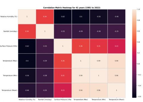
This study has conducted a correlation analysis among the parameters considered, namely Relative Humidity, Temperature (Max, Mean, Min), Surface Pressure, and Rainfall. The results, visualized using a heat map as shown in Figure 3, revealed intriguing relationships between these climate variables. The climate factors under the 41 years (1981 to 2022) study showed several strong relationships. Notably, the relationship between rainfall and humidity had a substantial positive correlation (r = 0.53), indicating that more rainfall likely to be accompanied by higher humidity levels. On the other hand, Surface Pressure (r = -0.67) and Temperature (Max) (r = -0.53) revealed considerable negative relationships with Relative Humidity (r = -0.53). This shows that maximum temperature and surface pressure tend to drop as relative humidity rises. Furthermore, a strong negative connection (r = -0.51) between rainfall and surface pressure was discovered, showing that larger rainfall totals correspond with lower surface pressure readings.
There is a minor tendency for relative humidity to rise when mean temperature rises, according to a weakly positive correlation between relative humidity and temperature (mean) that was found (r = 0.092). On the other hand, rainfall, and temperature (mean) showed a minor negative association (r = -0.2), indicating that larger rainfall levels are connected to marginally lower mean temperatures. Despite the existence of these connections, they are somewhat weak, suggesting that other factors may have a stronger impact on the associations between relative humidity and mean temperature as well as between rainfall and mean temperature. The reason to perform correlation analysis and generate the heat map was to collect the Pearson’s coefficient value (r) of different relationships between parameters and generate the trendline of 41 years how this relationship varies and its highest value and lowest value to confirm that particular year event and climatic variables trend.
Figure 3. Heatmap representation of Pearson coefficient (r) for daily timescale data of climatic variables for Koyna WLS from 1981 to 2022
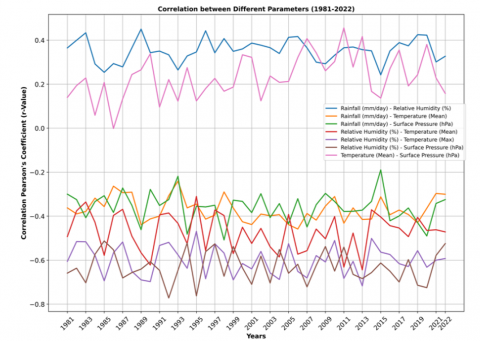
Figure 4. Line Plot Trend for Pearson coefficient (r) generated from Heatmap for the years from 1981 to 2022
The line plot in Figure 4 illustrates a notable decline in the correlation between Rainfall and Relative Humidity in the year 2015. Remarkably, this decline coincided with a period of reduced rainfall and drought-like conditions not only in the study region but also across the state of Maharashtra. In 2016, the correlation between Rainfall and Relative Humidity experienced a sudden increase and gradually continued to rise until 2019, reaching its highest strength. This upswing in the correlation aligned with the occurrence of a devastating flood in Western Maharashtra in the same year, 2019. The flood resulted from excessive rainfall, causing major districts like Satara, Sangli, and Kolhapur to be inundated as rivers overflowed. These findings suggest a potential link between the correlation patterns of Rainfall and Relative Humidity and the observed extreme weather events, highlighting the importance of understanding these relationships for climate monitoring and disaster preparedness.
3.3 Scatterplot for the years from 1981 to 2022 on daily timescale dataset
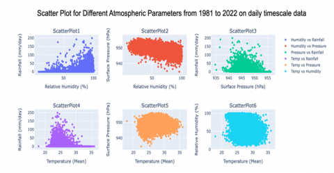
To gain insights into the relationship and trendline, Google Collab is used to generate scatter plots from a 41-year ERA5-Land dataset. The data, which has been assembled into a single file, has 15340 data points for each variable, allowing for a detailed evaluation of the interplay between the variables listed. These scatter plots help to validate the variables data values and its authenticity by understanding the theoretical predefined laws and relationship by practically generating scatterplots and check on the nature of relationship between two variables as they align with existing theory and teaching of atmospheric variables dependency.
For example, when the rainfall is expected, one of the favourable conditions is the high relative humidity, resulting a strong downpour which is experience in the daily interactions with climate. From Figure 5, scatterplot1 (Humidity vs Rainfall) denotes a directly proportional trend as relative humidity approaches 100%, the amount of rainfall also increases. However, it is crucial to note that relative humidity alone is not sufficient for rainfall to occur. Other factors, such as the formation of lowered pressure levels, play a significant role in precipitation events. In combination, these variables contribute to the conditions necessary for rainfall to occur. Scatterplot3 illustrates a pattern of higher rainfall associated with a decrease in pressure levels, while depicts that lower surface pressure corresponds to higher relative humidity percentages as seen in scatterplot 2. Scatterplots 2 and 3 display declining trend lines, indicating an inverse relationship between the variables. Specifically, as surface pressure levels decrease, rainfall tends to increase, and as surface pressure decreases, relative humidity tends to increase.
The dynamic relationship is observed in scatterplot4 between mean temperature and rainfall, as well as mean temperature and surface pressure in scatterplot 5. Higher rainfall is associated with a natural cooling effect on the atmosphere, leading to a decline in mean temperature. Conversely, lower surface pressure levels correspond to an increase in mean temperature. While scatterplot6 shows a constant trend between relative humidity and mean temperature. These figures demonstrate how changes in rainfall and surface pressure can influence mean temperature, contributing to the intricate interplay of these variables in the climate system.
Figure 5. Scatterplot for different atmospheric parameters from ERA5-Land dataset on daily timescale 1981 to 2022
3.4 ECWMF ERA5-land data plot
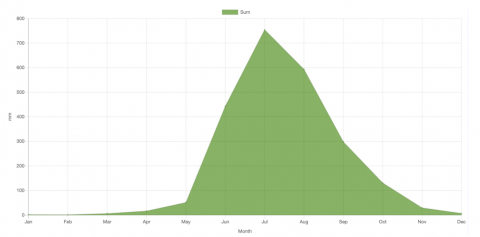
Figure 6 shows significant rise in rainfall pattern where year 2019 have shown highest rainfall on the other hand year 2015 shows a significant concerning drop in rainfall which was indeed a year of drought too. From Figure 7, the month of July receives highest rainfall and even seen lasting till October and slightly dropping in month of November. And hereby, there is extended rainfall, and October heat getting skipped since 2019.
Figure 6. Precipitation - ECMWF ERA5-Land daily 1981 to 2022
Figure 7. Precipitation monthly average- ECMWF ERA5-Land monthly 1981 to 2022
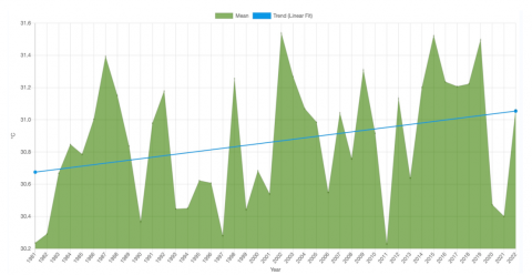
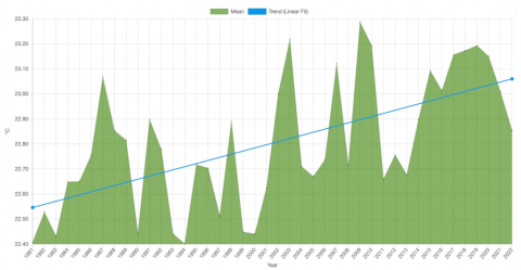
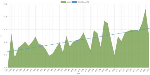
Figure 8a, Figure 8b and Figure 8c show a constant rise in all the temperature variables (maximum, minimum and mean respectively) indicating a significant turning point in the climate dynamics of the ECMWF ERA5-Land daily timescale dataset (1981-2022), particularly since 2019. Notably, the year 2019 had the highest annual rainfall of 3281.23mm, while the year 2015 had the lowest at 1655.11mm. Based on the monthly average of the daily timescale data, the trendline analysis shows an overall linear increase in rainfall, with July having the greatest average rainfall of 814.68mm. While Table 6 highlights the significant observations from the mentioned figures.
(a)
(b)
(c)
Figure 8. (a) Temperature- maximum (ECMWF ERA5- Land) 1981 to 2022; (b) Temperature- mean (ECMWF ERA5-Land) 1981 to 2022; (c) Temperature- Minimum (ECMWF ERA5-Land) 1981 to 2022
Table 6. Highlights from Figures 6-8 respectively of result for ECMWF ERA5-Land dataset from the year 1981 to 2022
|
Figure |
Significant Observations from ECMWF ERA-5 Land (1981-2022) |
Year/Month |
Rainfall (mm) |
Max Temp (℃) |
Mean Temp (℃) |
Min Temp (℃) |
|
6 |
Highest annual rainfall observed |
2019 2016 |
3281.23 3272.82 |
- |
- |
- |
|
6 |
Lowest annual rainfall observed |
2015 1987 |
1655.11 1512.84 |
- |
- |
- |
|
7 |
Month with highest average rain- fall |
July |
754.68 |
- |
- |
- |
|
8a |
Peak Annual Maximum Temperature observed |
2019 2015 2002 |
- - - |
31.55 31.50 31.54 |
- - - |
- - - |
|
8b |
Peak Annual Mean Temperature observed |
2019 2009 2003 |
- - - |
- - - |
23.19 23.29 23.22 |
- - - |
|
8c |
Peak Annual Minimum Temperature observed |
2021 2020 2009 |
- - - |
- - - |
- - - |
17.29 16.25 16.83 |
Furthermore, 2019 stands out as a year with a significant increase in maximum temperatures above the 35°C threshold. This rapid spike is concerning for the forest ecology, which often sees temperatures ranging from 24℃ to 25°C. Furthermore, the minimum temperature, which ranged from 15℃ to 18℃, increased significantly in 2019. Similarly, the maximum temperature climbed above 33℃. While all three temperature points show a linear increase, 2019 holds out with a sharp and rapid surge. These findings highlight the need of monitoring and comprehending climate change, particularly the significant changes reported in 2019, which may have ramifications for the forest ecology and local climate.
3.5 NASA GPM_3IMERGM v06 data plot
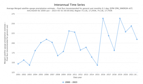
To cross validate the rainfall trend with ERA5-Land results, NASA GPM_3IMERGM v06 data from 2000 to 2022 is plotted.
(a)
(b)
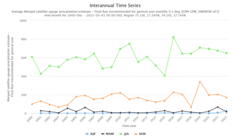
Figure 9. (a) GPM annual data (2000-2022); (b) GPM seasonal data (2000-2022)
Source: NASA Giovanni
Figure 9a using GPM data reveals a significant shift in the pattern of highest rainfall occurrences, particularly in the year 2019. Notably, a similar trend is observed, where 2015 recorded the least rain, followed by a sudden rise in 2016. Subsequently, in 2018, rainfall decreased again, though slightly higher than 2015, before spiking to the highest in 2019. The subsequent decline in 2020 suggests a cyclical pattern of high and low rainfall years, each with an equal interval of new values surpassing the previous ones. This emerging trend signals a potential change in the rainfall patterns, as indicated by the GPM merged satellite-gauge precipitation estimate final run. However, due to the availability of data only up to 2020, further trend analysis for 2021 and 2022 remains uncharted.
In Figure 9b, similar trend to Figure 9a is observed, reaffirming the cyclical pattern of rainfall variations. Particularly noteworthy is the consistency of June, July, and August (JJA) as the months with the highest rainfall, which aligns with the cyclical pattern seen in Figure 9a trend. This suggests that the cyclical fluctuations in rainfall are more pronounced during the JJA months, with these months consistently experiencing the highest levels of rainfall during the observed period. The overlapping trends in both figures further support the notion of a developing rainfall pattern and its association with specific months.
The discussion is focused on major part of findings from the results which is highlighted as below.
4.1 Year 2019 identified as significant year of climatic shift
From the results of monthly time scale dataset of ECMWF ERA5-Land and GPM _3IMERGM v06, it is found that year 2019 is observed to be a pivotal point from when the climate started getting more intense and it is seen that the variable like Rainfall is so changed, and downpour is indeed heavy for the month of October. It is the same year when western Maharashtra received devastating floods submerging the Sangli, Satara and Kolhapur districts, in August 2019. Significantly, the study's findings align with the discovery of a strong positive Indian Ocean Dipole phenomena in the same year, which stood out as one of the most powerful occurrences ever recorded. This reinforces the reliability and precision of the current study's results, which were acquired by examining climate patterns in 41 years or almost four decades of dataset.
4.2 October heat missing since 2019
The October heat event is identified as the retreating monsoon or transition season, this period denotes the shift from the rainy season to the colder, drier winter conditions. During this phase, the southwest monsoons gradually diminish and withdraw from the Indian subcontinent. The retreat of the monsoon is signified by a prevalence of clear skies and an increase in temperatures. While daytime experiences warmth, nights offer a refreshing coolness. The conjunction of elevated temperatures and humidity contributes to a climatic sensation that can be characterized as oppressive. To understand the trend of October Heat getting weakened, the recent few years of continuous trend is being identified by focusing on October month's data. The below Table 7 shows the average temperature and rainfall in the month of October from the year 2018 to 2022.
Table 7. Average rainfall and temperature values for the month October from year 2018 to 2022
|
Year |
Rainfall (mm) |
Temp (Max) ℃ |
Temp (Mean) ℃ |
Temp (Min) ℃ |
|
2018 |
82.91 |
33.78 |
27.89 |
22 |
|
2019 |
294.97 |
30 |
25.75 |
21.5 |
|
2020 |
287.42 |
30 |
25.55 |
21.1 |
|
2021 |
109.28 |
31 |
26 |
21.2 |
|
2022 |
263.55 |
30 |
25.3 |
20.6 |
The study uncovers a significant shift in climatic patterns, particularly observed since 2019 as seen in Table 8, where the extension of the Indian summer monsoon by an additional month has led to the omission of the October heat. Consequently, the usual transition to the winter season occurs without the occurrence of the typical October heating period. This emerging trend raises serious concerns due to the repercussions it brings. The surplus moisture in the soil results in runoff of nutrients and heightened soil erosion. This impact is not confined solely to forest ecosystems; it reverberates throughout agricultural ecosystems as well. The absence of the October heating process leaves the soil insufficiently dry, rendering it unsuitable for crop cultivation. The customary month-long drying and reduction of excess monsoonal moisture through October's heat are absent, forcing farmers to delay planting until a later month. Recently, winter crops are being sown as late as December, resulting in a subsequent delay in harvesting, which now coincides with the month of April—a time historically characterized by non-seasonal thunderstorms and rains. This convergence of delayed harvests and adverse weather conditions poses a substantial threat to the agriculture sector, precipitating considerable negative impacts.
4.3 Major findings from the result of trend analysis
Table 8 summarizes the main findings from the data of Koyna wildlife sanctuary, which focused on climatic trends as well as the identification of crucial periods that indicate shifts in weather patterns. The study uncovered significant disclosures by utilizing the ERA5-Land, and GPM data from earth observation satellites. However, it is vital to recognize the limitation caused by the lack of ground observatory, which limits the comparability of satellite-derived and ground data. In search of validation, the study's findings harmoniously coincide with historical happenings during the examined time frame. The study's findings are consistent with events such as the 2019 South Madhya Maharashtra floods, which were drove by a record-breaking positive Indian Ocean Dipole event, as well as the precise absence of October heat, which further validates satellite data through experiential verification.
Table 8. Key findings derived from this research study
|
Study Focus |
Key Findings |
|
Correlation Analysis |
Integration of Rainfall, Temperature, Relative Humidity, and Surface Pressure in Koyna WLS reveals significant correlations and trendline of the same. |
|
Impacted Weather Result |
Study highlights intensified weather patterns, emphasizing the complex interactions between climatic variables. Also, 2019 noticed highest rainfall and temperature resulting in devastating floods in South Madhya Maharashtra Region. |
|
Variable Trends (1981-2022) |
Overall increase in Rainfall, Max/Min/Mean Temperature; Sur- face Pressure remains stable; Relative Humidity is influenced by all other parameters, GPM Annual Rainfall data shows a significant trend pattern from 2015 till 2020. |
|
Turning Point - 2019 |
2019 marked intensified weather shift, linked with strong Indian Ocean Dipole (IOD) event and aligns with positive IOD observation, hence confirms the identified turning point with current methodology and more importantly, the October heat is skipped since 2019 and extension of rainfall in October is noticed. |
|
Implications for Ecosystem |
Atmospheric shifts may impact biodiversity, hydrology, and ecological equilibrium in the Koyna WLS. However, due to lack of October heat event, the soil remains wet, and winter starts resulting in lack of agricultural cultivation in order to wait for excess moisture dry out and the crop cycle has changed so far delayed by one month since 2019. |
|
October Heat |
Starting from 2019, the extended period of rainfall resulted to significant drop in temperature leading to omission of usual event of October heat that results to serious concerns over drying process of soil for a proper growth of forest as well as crop cultivation leading to presence of excess wetness of soil. |
|
Future Research and Mitigation |
The Trend Analysis Result findings establish ground- work for further study into climatic mechanisms; need for strategies to mitigate impacts |
4.4 Potential impact on Koyna WLS with corresponding to the factors identified from findings
Given the observed climate trends from the results, such as increased rainfall and temperature deviations, particularly since 2019, the Koyna Wildlife Sanctuary’s ecosystem could face significant alterations. These changes can impact both the abiotic and biotic components of the sanctuary's ecosystem.
Implications for Flora and Fauna
Table 9 shows the major climate change related factors that could possibly impact the region in different forms.
Table 9. Potential impacts of climate change-related factors on Koyna wildlife sanctuary
|
Identified Factor |
Potential Impact on Koyna WLS with Respect to Study Findings |
|
Intensified Weather Patterns |
Increased habitat disruption due to extreme weather. Stress on wildlife populations due to unpredictable conditions. |
|
Increased Rainfall |
Flooding of habitats and nesting sites. Changes in water availability and quality. |
|
Temperature Changes |
Shifts in vegetation and food availability for wildlife. Altered breeding and migration patterns. Impact on the various food chains. |
|
Absence of October Heat |
Disruption of soil drying process, affecting plant growth. Changes in cover and forage availability for wildlife. |
4.5 Dissecting the 2019 climatic shift: Causes and correlations within the Koyna wildlife sanctuary
The significant climatic shifts observed in 2019 within the Koyna Wildlife Sanctuary invite a detailed examination of the changes in climatic variables and the reasons behind these alterations. In this year, we note a pronounced deviation from established patterns, particularly with respect to rainfall and temperature dynamics, which coincides with extreme weather events affecting the Western Ghats region.
These shifts can be attributed to a complex interplay of local and global climatic drivers. The strong positive phase of the Indian Ocean Dipole (IOD) in 2019 is one such critical factor. The IOD, akin to El Niño in the Pacific, significantly influences the Indian monsoon system. A positive IOD typically leads to increased rainfall in the Northwestern Indian Ocean region or Arabian Sea, which corresponds with the amplified precipitation recorded in the sanctuary.
The unusually prolonged monsoon season, extending into October, can be linked to delayed monsoon retreat, a phenomenon that has been increasingly observed in recent years. Studies suggest that rising global temperatures may be contributing to this pattern, as warmer air and ocean temperatures can alter atmospheric circulation and extend the monsoon period.
The data from 2019 thus serves as a case study for understanding the sanctuary's vulnerability to climatic variations and underscores the necessity for dynamic conservation strategies that can adapt to these changes. Ongoing research and monitoring are essential to predict and mitigate the long-term impacts of such climatic anomalies on the sanctuary's delicate ecosystems.
4.6 Future scope on current research extension
Table 10 provides a future scope of study's extension that can be planned based on present study outcomes.
Table 10. Future scope in extending the study using the present research outcome
|
Future Scope in Extending Study |
Description |
|
Climate Change Adaptation Strategies |
Conduct research to develop specific climate change adaptation strategies for the sanctuary, including habitat restoration and management practices to mitigate the impacts of intensified weather patterns and track wildlife behaviour towards changing climate and their response in adapting the changes. |
|
Meteorological Observatory Stations |
Having a ground observatory to monitor the climate and store daily timescale activities data will help to validate the satellite data and study the both results. |
|
Community Engagement and Education |
Engage with local communities and raise awareness about cli- mate change impacts on the sanctuary. Collaborate with com- munities on sustainable land use practices and conservation efforts. |
The findings of this study have centred on the examination of long-term climatic trends of dataset of the one of biodiversity hotspot, Koyna Wildlife Sanctuary (WLS), encompassing variables such as Rainfall, Temperature, Relative Humidity, and Surface Pressure. The methodology employed offers a sophisticated framework for undertaking analogous climatic trend analyses in diverse biodiversity hotspots that currently lack such investigations. Importantly, this approach is not restricted solely to the specific sites but can be universally applied to all biodiversity hotspots. In instances where ground observation data is scarce, the study emphasizes the use of experiential validation through a retrospective examination of past events within the biodiversity hotspot. This methodology holds promise for enhancing our understanding of climatic trends in various ecological and biodiversity hotspots worldwide.
During the analysed period from 1981 to 2022, the data of an area under study exhibited a general rise in the average values of Rainfall and Temperature (Max, Min, Mean). In contrast, Surface Pressure remained relatively consistent, exhibiting no notable fluctuations. Relative Humidity, on the other hand, displayed a stronger dependency on Rainfall, Surface Pressure, and Maximum Temperature, collectively affecting its fluctuations.
Interestingly, the year 2015 experienced a weaken annual trend of Pearson coefficient (r) correlations. This indicated a decline in the interplay between the climatic variables during that period, which resembles a pattern observed back in 1987. In contrast, the year 2019 displayed a stronger trend in the interplay between the variables with highest annual rainfall of 3281.23mm throughout the 41 years of time span. This figure even slightly surpassed the annual rainfall of 3272.82mm recorded in 2006.
In 2019, significant changes in weather patterns occurred in the Koyna WLS, potentially impacting biodiversity, hydrology, and ecological balance as what South-western Maharashtra State experienced in 2019 Floods. These findings are consistent with a strong positive phase of the Indian Ocean Dipole (IOD), one of the strongest in historical records, validating the study's reliability. Additionally, the prolonged Indian summer monsoon since 2019, leading to the absence of the October heat transition, which now may pose a risk for ecosystems, agriculture, and soil conditions due to disrupted climate patterns.
This study's findings on climatic trends in the Koyna Wildlife Sanctuary are subject to limitations, notably the lack of long-term ground observation data, which could enhance the precision of satellite-derived measurements. The use of retrospective event analysis, while insightful, cannot replace the subtle understanding that continuous on-site monitoring would provide. Additionally, the resolution of satellite data may not fully capture the microclimatic diversity of the sanctuary's ecosystem. Future research would benefit from integrating higher-resolution ground data to validate and refine these findings, addressing the potential non-stationarity in climate behavior and its implications for the sanctuary's biodiversity.
Despite this constraint impacting the depth of this trend analysis, the research findings represent a crucial advancement in comprehending the changing climatic patterns within the biodiversity hotspot throughout the experiential validation of climatic events occurred in past. This additional data source will provide valuable ground-based insights. The present study remains of great importance, serving not only Koyna WLS but also as a valuable model for investigating climatic trends of various protected areas through a similar approach.
|
% |
Percent |
|
℃ |
Degree Celsius |
|
r |
Pearson's Coefficient of Correlation |
|
α |
Mann-Kendall trend test's significance level |
|
β |
Sen’s Slope |
|
mm |
Millimeters |
|
C3S |
Copernicus Climate Change Service |
|
ECMWF |
European Centre for Medium-Range Weather Forecasts |
|
ERA5 |
ECMWF Re-Analysis 5 |
|
Giovanni |
Geospatial Interactive Online Visualization ANd aNalysis Infrastructure |
|
GPM |
Global Precipitation Measurement |
|
hPa |
Hectopascal |
|
IMERG |
Integrated Multi-satellitE Retrievals for GPM |
|
IOD |
Indian Ocean Dipole |
|
IPCC COP27 |
Intergovernmental Panel on Climate Change 27th Conference of the Parties |
|
IUCN |
International Union for Conservation of Nature |
|
Max |
Maximum |
|
Min |
Minimum |
|
NASA |
National Aeronautics and Space Administration |
|
NOAA |
National Oceanic and Atmospheric Administration |
|
PMEL/TMAP NOAA |
Pacific Marine Environmental Laboratory's Thermal Modeling and Analysis Project |
[1] Pörtner, H.O., Roberts, D.C., Tignor, M.M.B., et al. (2022). Climate change 2022: Impacts, adaptation and vulnerability working group II contribution to the sixth assessment report of the Intergovernmental Panel on Climate Change. Cambridge University Press. https://doi.org/10.1017/9781009325844.
[2] Vose, J.M., Peterson, D.L., Domke, G.M., et. al. (2018). Forests. In: Impacts, Risks, and Adaptation in the United States: Fourth National Climate Assessment, Volume II, U.S. Global Change Research Program, pp. 232-267. https://doi.org/10.7930/NCA4.2018.CH6
[3] Nandargi, S., Mulye, S. (2012). Relationships between rainy days, mean daily intensity, and seasonal rainfall over the Koyna catchment during 1961–2005. The Scientific World Journal, 2012: 894313. https://doi.org/10.1100/2012/894313
[4] Jha, S., Bharti, B., Reddy, D.V., Shahdeo, P., Das, J. (2020). Assessment of climate warming in the Western Ghats of India in the past century using geothermal records. Theoretical and Applied Climatology, 142: 453-465. https://doi.org/10.1007/s00704-020-03321-1
[5] Bajirao, T.S., Kumari, A., Changade, N.M. (2023). Applicability of geospatial technology for drainage and hypsometric analysis of Koyna River Basin, India. In: Surface and Groundwater Resources Development and Management in Semi-arid Region, pp. 225-252. https://doi.org/10.1007/978-3-031-29394-8_13
[6] Patil, J., Shinde-Pawar, M., Kanthe, R. (2020). Flood disasters 2019 in Maharashtra (India), aftermath and revival for natives and tourists. Ecology, Environment and Conservation, 26(2): 693-698.
[7] Jothiprakash, V., Fathima, T.A. (2013). Chaotic analysis of daily rainfall series in Koyna reservoir catchment area, India. Stochastic Environmental Research and Risk Assessment, 27: 1371-1381. https://doi.org/10.1007/s00477-012-0673-y
[8] Vadnere, N. (2019). Expert study committee report: Floods 2019 (Krishna Basin). Water Resource Department, Government of Maharashtra, India. https://wrd.maharashtra.gov.in/Upload/PDF/Vol%201%20Main%20Report.pdf, accessed on Feb. 22, 2024.
[9] Ratna, S.B., Cherchi, A., Osborn, T.J., Joshi, M., Uppara, U. (2021). The extreme positive Indian Ocean dipole of 2019 and associated Indian summer monsoon rainfall response. Geophysical Research Letters, 48(2): e2020GL091497. https://doi.org/10.1029/2020GL091497
[10] Meet ENSO’s neighbor, the Indian ocean dipole. https://www.climate.gov/news-features/blogs/enso/meet-enso’s-neighbor-indian-ocean-dipole, accessed on Feb. 22, 2024.
[11] UNESCOWHC. (2012). Western Ghats. https://whc.unesco.org/en/list/1342/, accessed on Feb. 22, 2024.
[12] Molur, S., Smith, K., Daniel, B., Darwall, W. (2011). The Status and Distribution of Freshwater Biodiversity in the Western Ghats, India. IUCN, Cambridge, UK and Gland, Switzerland.
[13] Joglekar, A., Tadwalkar, M., Mhaskar, M., Chavan, B., Ganeshaiah, K.N., Patwardhan, A. (2015). Tree species composition in Koyna Wildlife Sanctuary, Northern Western Ghats of India. Current Science, 108(9): 1688-1693.
[14] Muñoz-Sabater, J.; Dutra, E.; Agustí-Panareda, A., et al. (2021). ERA5-land: A state-of-the-art global reanalysis dataset for land applications. Earth System Science Data, 13: 4349-4383. https://doi.org/10.5194/essd-13-4349-2021
[15] Huffman, G., Stocker, E., Bolvin, D., Nelkin, E., Tan, J. (2019). GPM IMERG final precipitation L3 1 day 0.1 degree x 0.1 degree V06. Goddard Earth Sciences Data and Information Services Center (GES DISC). https://doi.org/10.5067/GPM/IMERGDF/DAY/06
[16] Liu, Z., Acker, J. (2017). Giovanni-The bridge between data and science. GSFC-E-DAA-TN43547, Goddard Space Flight Center.
[17] Warren, J. (1988). Statistical methods for environmental pollution monitoring. Technometrics, 30(3): 348. https://doi.org/10.1080/00401706.1988.10488409
[18] Kendall, M. (1955). Rank Correlation Methods. 2nd impression. Charles Griffin and Company Ltd. London and High Wycombe.
[19] Mann, H. (1945). Non-parametric tests against trend. Econometria, 13(3): 245-259. https://doi.org/10.2307/1907187
[20] Liu, Z., Cuo, L., Li, Q., Liu, X., Ma, X., Liang, L., Ding, J. (2020). Impacts of climate change and land use/cover change on streamflow in Beichuan River Basin in Qinghai Province, China. Water, 12(4): 1198. https://doi.org/10.3390/w12041198
[21] Sen, P.K. (1968). Estimates of the regression coefficient based on Kendall’s tau. Journal of the American Statistical Association, 63(324): 1379-1389. https://doi.org/10.1080/01621459.1968.10480934
[22] Liu, H. (2021). Wind Forecasting in Railway Engineering. Elsevier.