Dheyaa Hamdan Dagher*![]() | Imad Habeeb Obead
| Imad Habeeb Obead![]()
© 2023 IIETA. This article is published by IIETA and is licensed under the CC BY 4.0 license (http://creativecommons.org/licenses/by/4.0/).
OPEN ACCESS
In this study, the Discrete Differential Dynamic Programming (DDDP) method is utilized to identify the optimum rule curves and policies for the Tharthar Reservoir by adopting an objective function to reduce the release and storage losses. The input data for the optimization model represents the historical data for the Tharthar Reservoir within the Euphrates River Basin from October 2000 to September 2021. The years within this period will be categorized as two sequential wet and dry years for the reservoir operation through the development period of October 2022 to September 2059. In the first scenario, TH1, the plan is unsafe during the planning period of the operation because there is a high deficit in storage and outflow. The summation of the deficit in storage and outflow after applying the TH1 scenario is equal to 52671 million cubic meters (MCM). The second scenario, TH2, is an alternative scenario for operating the Tharthar Reservoir. The summation deficits from using TH2 are equal to 13071 MCM for storage and outflow. The results simulated for the monthly storage were compared with the measured data for a reliability test. Also, the projected water supply calculated by the optimization model by DDDP was compared with the WEAP model. From this comparison, the three statistical parameters, R2, NSE, and RSR, were evaluated as an acceptable level and a good agreement of the DDDP and WEAP model performance.
curve rule, Discrete Differential Dynamic Programming, optimal operation, Tharthar Reservoir, Water Evaluation and Planning
Water resource systems have helped both people and economies. These systems offer a wide range of services. Nevertheless, in many parts of the world, they cannot meet even the most basic drinking water and sanitation needs [1]. The Euphrates flow has evolved to have less noticeable seasonal variations due to the installation of major hydraulic engineering works upstream from Turkey and Syria. Irrigation, hydroelectricity, and drinking water are the primary uses of water in the Euphrates River Basin (ERB) in Iraq, Syria, and Turkey, with agriculture absorbing more than 70% of the water [2]. This problem to be more severe in the future when the supply is 43 and 17.61 billion Cubic Meters (BCM) in 2015 and 2025, respectively. At the same time, current demand is estimated to be between 66.8 and 77 BCM [3]. Turkey has launched an ambitious plan to develop the GAP project in this context. Therefore, the lower riparian countries (Syria and Iraq) are experiencing problems of water scarcity and deteriorating water quality [4].
Discrete Differential Dynamic Programming (DDDP) is a computational method to obtain the solution to optimization problems [5]. Murray and Yakowitz [6] described and evaluated sequential approximation dynamic programming approaches. This approach effectively solved multi-reservoir control difficulties. A particular control problem aims to develop a strategy that satisfies the requirements and minimizes the loss function. Also, Murray and Yakowitz [7] proposed a comparison between the second-order method known as differential dynamic programming DDP and Newton's method, known as unconstrained discrete-time optimal control problems. Al-Delewy et al. [8] implemented the DDDP technique to adopt an objective function to minimize the release and storage penalty. Mohammed [9] used the DDDP approach to find the optimal monthly operation of Haditha Dam by adopting an objective function to minimize the release and storage penalty. Al-Mansori [10] used the DDDP to find the best optimal policy for the monthly operation of Haditha Reservoir for 24 years to minimize the total penalties taken place due to both releases and storage when exceeded by the limited allowable values. Ali and Abed [11] used the DDDP approach and simulation model to find the optimal monthly operation of Ilisu Dam. Also, found the optimum monthly release and storage by adopting an objective function that minimizes the release and storage losses (penalty).
Avarideh et al. [12] showed that to simulate the basin, Water Evaluation and Planning (WEAP) is a professional engineering tool for water resources planning. AlMohseen and Klari [13] designed a management strategy using the WEAP model. Sameer et al. [14] developed a sustainable water resource management approach in the upper ERB to extend the year 2035 using the WEAP model. Noon et al. [15] used the WEAP software to estimate the amount of water unmet demand and demand in the future for cities in the Anbar province of Iraq. Al-Mukhtar and Mutar [16] used the WEAP software to evaluate and analyze Baghdad province's current and future balance of water resources management. Sharef et al. [17] analyzed the optimal planning system and operational policies for Iraq's Great Zab Basin (GZRB) using the WEAP model.
From the literature review, most water management studies in the Tigris and Euphrates River Basin have yet to focus on the optimal operation of Tharthar Reservoir. This research includes a solution for the problem of the optimal operation of the Tharthar Reservoir. This solution is based on an analysis of the multi-purpose and multi-stage approach for Tharthar Reservoir. Many factors have been considered in finding the optimal operation, including urban, agricultural, and industrial expansion, as well as the impact of climate change. The planning period for water management extends from October 2022 to September 2059.
2.1 The study area
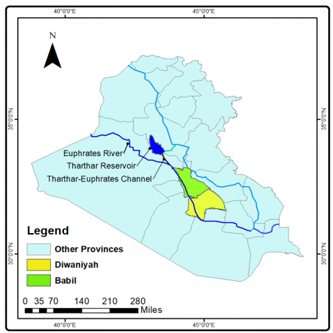
Tharthar Reservoir is one of the largest closed depressions in Iraq; it is in the central western part of Iraq, between the Jazira and Mesopotamia Plains, west of the Tigris River [18]. The regulator of Tharthar-Euphrates Channel has four gates with dimensions of (8 m×7 m) and a discharge of 500 m3/s. The Tharthar-Euphrates Channel, which meets the Euphrates River close to Habbaniyah city, is under the supervision of this regulator. Tharthar-Euphrates Channel is 26.8 kilometers long and was initially used to move water to the Euphrates River in 1976 [19]. In this study, Tharthar Reservoir supplied water for both Babil and Diwaniyah provinces in Iraq. A layout map for study areas is shown in Figure 1. Babil province is in central Iraq, south of Baghdad, the Longitudes (43° 58' 10") and (44° 38' 35") east of Greenwich and Latitudes (32° 7' 25") and (33° 0' 35") north of the Equator [20]. Diwaniyah province is located between longitudes (44° 42' 0") and (44° 27' 0") and two latitudes (31° 45' 0") and (32° 45' 0") [21].
Figure 1. Layout map for the study area, the source of the shape files is (www.diva-gis.org/gdata)
Figure 2. Illustration of dynamic programming mechanism for reservoir operation, adopted from the study [22]
2.2 Formulation of the optimization model
At each stage t, a decision Rt must be made to move to the next stage (t+1), linked by a transition-state equation, i.e., the mass balance Equation. Each decision depends on the system's current state, defined by the vector of state variables St. A sequence of optimal decisions constitutes an optimal policy [23]. This procedure is illustrated in Figure 2 in the context of reservoir operation.
The problem characteristic mentioned above, ft can be defined as a transformation function that acts on the state vector St to convert it into a state vector St+1 associated with the stage (t+1), because of the action of the decision vector in the Rt in the t stage expressing in mathematical terms:
$S_{t+1}=f_t\left(S_t, R_t\right)$ where, $t=1,2, \ldots N$ (1)
Consider that Eq. (1) is the dynamic system equation. For example, in a network of reservoirs, the state refers to the storage, and the decision refers to the release from storage [5]. The objective function to be maximized is:
$\mathrm{F}=\sum_{\mathrm{t}=1}^{\mathrm{N}} \mathrm{R}\left(\mathrm{S}_{\mathrm{t}}, \mathrm{R}_{\mathrm{t}}\right)$ (2)
where, F is the sum of returns from the system over the time horizon and $R\left(S_t, R_t\right)$ is the return of a decision Rt. The performance criterion to be maximized is the sum of the returns due to power generated by the power plants and the return from the diversion of Rt.
$F_t=\sum_{t=1}^N b_t\left(R_t\right)+\sum_{t=1}^N g_t\left[\left(S_t\right),\left(a_t\right)\right]$ (3)
where, $F_t$ is the total return from the system, $t=1,2, \ldots \mathrm{N}, b_t$ is the unit returned due to a decision $R_t$ during a period starting at stage $t$ and lasting until stage $(\mathrm{t}+1)$, and $g_t\left[\left(S_t\right),\left(a_t\right)\right]$ is a function that assesses a penalty to the system, at is the desired state [24].
An optimization model constitutes the objective function and the set of imposed constraints. For the operation of a reservoir, the constraints are commonly storage constraints, release constraints, and continuity constraints. For the case study, the following constraints are valid:
1. Storage constraint: The storage at the start of the first operation period should be a known quantity. However, storage in other periods should be within the set of allowable limits as specified by the design criteria of the dam. That is:
$\operatorname{Min} . \mathrm{S} \leq \mathrm{S}_{\mathrm{t}} \leq \operatorname{Max} . \mathrm{S}$ (4)
Min.S and Max.S are the minimum and maximum limits of storage, respectively; St is the storage sequence; t is the serial number of the denoting months, t=1, 2, 3 …, N [25].
2. Release constraint: The release during the t month should be within the range of feasible limits, that is:
Min. $\mathrm{PF} \leq \mathrm{R}_{\mathrm{t}} \leq \mathrm{Max}$. PF (5)
where, Rt is the release from the reservoir during t month, Min.PF is the minimum permissible flow downstream of the reservoir, and Max.PF is the maximum permissible flow downstream of the reservoir.
IF $R_t \leq 0$, then $R_t=0$ (6)
Otherwise, $\mathrm{R}_{\mathrm{t}}=\mathrm{D} \mathrm{e}_{\mathrm{t}}$ (7)
where, $D e_t$ is the monthly demand, and Min.PF equals zero.
3. Continuity constraint: Continuity constraints consider the transfer of the reservoir storage from the beginning of one period to the beginning of the next. The inflow-outflow indicates the activity of the reservoir and can be represented as:
$S_{t+1}=S_t+Q_t-E v_t+P r_t-R_t$ (8)
where, are all in consistent units: $R_t$ is the reservoir release, $P r_t$ is the precipitation on the reservoir, $E v_t$ is the evaporation from the reservoir, and $Q_t$ is the reservoir inflow [25].
4. The water quality constraint considers the TDS as the major controlling parameter, the constraint of the salt concentration of the water released from the reservoir can be represented as:
$\text{IF TDS}_t>$ MA.TDS, then $R_t=0$ (9)
$T D S_t$ is the total dissolved solid of the reservoir water during the t month (mg/L), and MA. TDS is the maximum allowable Total Dissolved Solid.
The two operation decisions rule can be represented in two cases the deficit in the dry year and the spillage in the wet year. To derive the objective functions for calculating total losses due to storage and release by modifying Eq. (3) and Eq. (4), this could be represented as follows:
1. The spillage losses case:
$\operatorname{Minimize}(\mathrm{TLS})=\sum_{\mathrm{t}=1}^{\mathrm{N}} \mathrm{L}\left(\mathrm{S}_{\mathrm{t}+1}\right)$ (10)
where, TLS is total Spillage losses, $L\left(S_{t+1}\right)$ is the loss function of the storage. The objective function of the spillage case subject to:
If $S_{t+1}>($ Max $S)$ then, $L\left(S_{t+1}\right)=S_{t+1}-\text{Max S}$ (11)
Otherwise, $\mathrm{L}\left(\mathrm{S}_{\mathrm{t}+1}\right)=0$ (12)
2. The deficit case:
$\operatorname{Minimize}(T D)=\sum_{t=1}^N D\left(S_{t+1}\right)$ (13)
where, TD is the total Deficit of the storage, and $D\left(S_{t+1}\right)$ is the deficit function of the storage. The objective function of the deficit case is subject to the following:
If $\mathrm{S}_{\mathrm{t+1}+1}<\mathrm{Min} . \mathrm{S}$ then, $\mathrm{D}\left(\mathrm{S}_{\mathrm{t+1}}\right)=\mathrm{S}_{\mathrm{t}+1}-\mathrm{Min} . \mathrm{S}$ (14)
Otherwise, $\mathrm{D}\left(\mathrm{S}_{\mathrm{t+1}}\right)=0$ (15)
In the objective function of release, the aim is to minimize the defect associated with a failure in supplying the demand, no less or more is set as the following:
1. (Spillage losses) case:
Minimize TLR$ =\sum_{t=1}^N L\left(R_t\right)$ (16)
where, TLR is the total losses due to release; $L\left(R_t\right)$ is the loss function of the release in the t month.
If $R_t>D e_t$ then, $L\left(R_t\right)=R_t-D e_t$ (17)
Otherwise, $L\left(R_t\right)=0$ (18)
If $R_t>$ Max. PF then $L\left(R_t\right)=R_t-$ Max.PF (19)
Otherwise, $L\left(R_t\right)=0$ (20)
2. Deficit losses case:
$\operatorname{Minimize}(T D)=\sum_{t=1}^N D\left(R_t\right)$ (21)
If $R_t<\mathrm{De}_t$ then $\mathrm{L}\left(\mathrm{R}_{\mathrm{t}}\right)=\mathrm{R}_{\mathrm{t}}-\mathrm{De}_{\mathrm{t}}$ (22)
Otherwise, $L\left(R_t\right)=0$ (23)
If $R_t<$ Max. PF then $L\left(R_t\right)=R_t-$ Max.PF (24)
Otherwise, $L\left(R_t\right)=0$ (25)
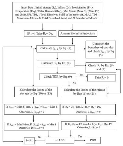
where, TD is the total deficit of the storage, and $D\left(R_t\right)$ is the deficit function of the storage. Figure 3 shows the flowchart of the methodology for the optimization model. The current study uses the DDDP method to solve an optimization problem in the Microsoft Excel Visual Basic Application VBA.WEAP employs LP Solver, an open-source linear program solver. The WEAP Model can be used to calculate the optimal outflow and compare it with the outflow of the optimization model.
Figure 3. The flowchart of the methodology for the optimization model
2.3 The estimation of the water demand
The total water demand included the agricultural, municipal, and industrial sectors. The methodology of the estimation of the water demand can be adopted as a following:
1. The irrigation demand: CROPWAT software depends on the climatic data to calculate the monthly and annual reference evapotranspiration by applying the Penman-Monteith. The Penman-Monteith method is selected as the method by which the evapotranspiration of this reference surface (ETo) can be determined [26]. This method of estimation can be expressed as follows:
$\mathrm{ETo}=\frac{0.408 \Delta\left(\mathrm{R}_{\mathrm{n}}-\mathrm{G}\right)+\gamma\left(\frac{900}{\mathrm{~T}+273}\,\,\,\right) \mathrm{u}_2\left(\mathrm{e}_{\mathrm{s}}-\mathrm{e}_{\mathrm{a}}\right)}{\Delta+\gamma\left(1+0.34 \mathrm{u}_2\right)}$ (26)
where, $R_n$ is the net radiation at the crop surface $\mathrm{MJ} / \mathrm{m}^2$ day, $\mathrm{G}$ is the soil heat flux density $\mathrm{MJ} / \mathrm{m}^2$ day, $\mathrm{T}$ is the mean daily air temperature at $2 \mathrm{~m}$ height ${ }^{\circ} \mathrm{C}, \mathrm{u}_2$ is the wind speed at $2 \mathrm{~m}$ height $\mathrm{m} / \mathrm{s}, e_s$ is the saturation vapour pressure $\mathrm{KP}_{\mathrm{a}}, e_a$ is the actual vapour pressure $\left(\mathrm{KP}_{\mathrm{a}}\right),\left(e_s-e_a\right)$ is the saturation vapor pressure deficit $\left(\mathrm{KP}_{\mathrm{a}}\right), \Delta$ is the slope vapor pressure curve $\left(\mathrm{KP}_{\mathrm{a}} /{ }^{\circ} \mathrm{C}\right), \gamma$ is the psychrometric constant $\left(\mathrm{KP}_{\mathrm{a}} /{ }^{\circ} \mathrm{C}\right)$. The equation of crop evapotranspiration can be represented mathematically as the following:
$\mathrm{ETc}=\mathrm{Kc} * \mathrm{ETc}$ (27)
where, ETc crop evapotranspiration (mm/day), Kc crop coefficient [26]. Net irrigation water requirements (NIWR) are determined by using the formula:
$\mathrm{NIWR}=\mathrm{ET} \mathrm{c}-\mathrm{Re}$ (28)
where, Re is the effective rainfall [27].
The data for CROPWAT used in calculating crop irrigation water demand in Babil and Diwaniyah provinces was taken from the research by Allen et al. [26]. The three scenarios of climate change data RP, SSP1-2.6, and SSP2-4.5 were used in the calculation. The net irrigation areas for Babil and Diwaniyah are 345675 and 248978 hectares, respectively. A total of 32 seasonal and annual crops, including wheat, barley, vegetables, rice, and citrus, were planted in the provinces of Babil and Diwaniyah [20].
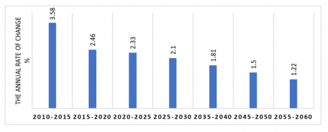
2. The municipal demand: United Nations [28] projected the population percentage rate for 197 nations, including Iraq, using models based on the evolution of the fertility rate in each region. Figure 4 shows the annual percentage rate of change of the population growth in the Babil and Diwaniyah provinces.
The last census in Iraq was carried out in 1997; after that date, only estimates were provided by government offices, namely the Ministry of Planning. Based on these values, the overall Iraqi population trends have been examined, and the early growth rates have been calculated. In 2013, the Republic of Iraq Ministry of Planning (RIMP) conducted population estimates in 2009 based on the 1997 Census. Table 1 shows the population of the provinces that lie in the Euphrates River Basin. Table 2 can calculate the number of residents in the Babil and Diwaniyah provinces, including the period of the development manager for the Euphrates River Basin.
Figure 4. The percentage rate of population growth [28]
Table 1. Number of the resident of the Babil and Diwnaiyah provinces in 2009 [29]
|
Province |
The Number of the Resident |
|
Babil |
1729666 |
|
Diwaniyah |
1077614 |
Table 2. Projection the number of the resident in the Babil and Diwnaiyah provinces from 2009 to 2060
|
|
The Number of the Resident |
||||||
|
Year |
2009 |
2020 |
2025 |
2035 |
2045 |
2055 |
2060 |
|
Babil |
1729666 |
2290107 |
2556905 |
3093855 |
3653842 |
4201919 |
4458236 |
|
Diwaniyah |
1077614 |
1426779 |
1592999 |
1927529 |
2276412 |
2617873 |
2777564 |
Ministry of Water Resources (MoWR), considering the design capacity of each Water Treatment Plant (WTP) and Compact Water Treatment Plant (CU). Generally, the WTPs belong to main cities, while the CWTPs are associated with districts and subdistricts. Their treatment capacities vary according to the population served. Table 3 shows the actual capacity of WTPs and CU for Babil and Diwaniyah [30].
3. Industrial demand: In general, water quality and quantity for industrial consumption vary with the type of industry. In Iraq, the industrial water demand can be divided into oil fields and refineries, which are relevant to the Ministry of Oil, thermo-power plants, which the Ministry of Electricity controls, and other industries, mainly under the supervision of the Ministry of Industry. The industrial water consumption data were retrieved from the study entitled "Strategy for Water and Land Resources in Iraq" (SWLRI), which was prepared for the Iraqi Ministry of Water Resources [30]. The water consumption for Iraq's provinces was estimated in the [31] for the years 2010, 2015, 2020, 2025, 2030, and 2035 [30]. Table 4 shows the final projected industrial sectors for the Babil and Diwaniyah water withdrawals.
Table 3. The actual capacity of (WTPs) and (CU) of the Babil and Diwnaiyah provinces [30]
|
Actual Capacity (m3/d) |
|||
|
Governorate |
WTP |
CU |
Total |
|
Babil |
245920 |
502408 |
748328 |
|
Diwaniyah |
198773 |
188531 |
387304 |
Table 4. The projected industrial water demand (m3/d) [30]
|
Governorate |
2010 |
2015 |
2020 |
2025 |
2030 |
2035 |
|
Babil |
19781 |
29672 |
39563 |
49453 |
59344 |
69235 |
|
Diwaniyah |
1713 |
2.569 |
3425 |
4282 |
5138 |
5994 |
Table 5. The basic data of Tharthar Reservoir
|
Storage in Reservoir (MCM) |
Value |
Reservoir Water Level (m.a.s.l) |
Value |
|
Maximum Design Storage |
85000 |
Maximum Design level |
65 |
|
Maximum operated Storage |
82930 |
Maximum operated level |
59.11 |
|
Minimum operated Storage |
39560 |
Minimum operated level |
41.83 |
|
Dead Storage |
39600 |
Top Level of Dead Storage |
42.5 |
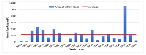
Figure 5. The annual inflow rate of the Tharthar Reservoir
2.4 The salinity problem of the ERB
There has been a decline in river flow on the Euphrates, which is most noticeable upstream. On the other hand, the river flow is not expected to decrease in the middle and downstream sections of the river. Total dissolved solids (TDS) values less than 600mg/l are typically considered good for water palatability; drinking water becomes considerably more unpleasant at TDS levels beyond 1000mg/l [32]. The TDS data's source is NCFWRM [33]. The data on the TDS for Tharthar Reservoir is only available for 2020-2022, during which time the average value of the TDS was 781mg/l. The average of the maximum allowable TDS (MA.TDS) for drinking water and irrigation water requirements (1000mg/l) can be used to suggest the MA.TDS.
2.5 The basic data of Tharthar Reservoir
The operation rule curve of the Tharthar Reservoir can be derived from the available storage and elevation records from October 2000 to September 2020 by NCFWRM [33]. The basic data of the Tharthar Reservoir are briefly shown in Table 5. According to this, data can be adopted to construct the water surface elevation (WSE)-storage relation.
Tharthar Reservoir can be selected the exponential trendline to derive the equations of the Storage-WSE relation because of a good accuracy for the reliability by using the coefficient of determination. Additionally, the predicted values of WSE are located between the maximum and minimum WSE. The mathematical equation for the average of the Storage-WSE of the Tharthar Reservoir is:
The mathematical equation for the average of the (Elevation-Storage) of the reservoir is as follows:
El=13.208 e3E-05S (29)
The equation of the maximum WSE-Storage of the Tharthar Reservoir is:
El=25.143 e1E-05S (30)
The equation of the minimum (WSE-Storage) of the Tharthar Reservoir is:
El = 15.56 e2E-05S (31)
where, S is the storage of the Tharthar Reservoir.
2.6 Selected scenarios for the operation
Based on available data from October 2000 to September 2021 by NCFWRM [33]. Figure 5 shows the average annual inflow rate for Tharthar Reservoir. The main scenarios for the operation of the reservoirs can be determined based on the inflow. From the annual inflow rate analysis, the assumption is that any value greater than average can be considered a "wet year", and less than average is a "dry year". The other scenario of Tharthar Reservoir is that the TH1 scenario depends on reducing the agricultural demand to 50%. As a result of the high deficiency, scenario TH2 is an alternative scenario for operating the Tharthar Reservoir, and it includes drawing water from the reservoir's dead storage. Therefore, Iraq's Ministry of Water Resources (MoWR) has put floating pumping stations on the dead storage to capitalize on the drought periods. When the storage in the conservation zone is depleted, Tharthar's dead storage, equal to 39600 MCM, can be used.
2.7 Evaluation criteria
The last step in their application will be to evaluate the performance of a measurement system after projecting the climate change data and simulating the agricultural model using CROPWAT Model. Some of the fundamental statistics for Calibration and Verification measures are as follows:
1. Coefficient of determination (R2): Describes the proportion of the variance in measured data explained by the model. R2 ranges from 0 to 1, with higher values indicating less error variance, and typically values greater than 0.5 are considered acceptable [34]. (R2) is used to evaluate the results of the calibration and validation of the model [35]. With the assistance of Microsoft Excel, (R2) was graphically derived.
2. Nash-Sutcliffe efficiency (NSE): The Nash-Sutcliffe coefficient (NSE), also called the coefficient of efficiency, indicates how well the plot of observed versus simulated data is close to the 1:1 (equal value) line. The Nash-Sutcliffe coefficient is like the coefficient of determination. However, instead of using the linear regression line of best fit, (NSE) compares the observed values to the 1:1 line of measured versus predicted data [36]. The Nash-Sutcliffe efficiency evaluates the conformance between simulated and observed data [35]. (NSE) is computed as shown in the following equation:
$\mathrm{NSE}=1-\frac{\sum_{i=1}^n\left(X_{o b s}-X_{s i m}\right)^2}{\sum_{i=1}^n\left(X_{o b s}-\bar{X}_{o b s}\right)^2}$ (32)
NSE ranges between−∞ and 1.0 (1 inclusive), with NSE=1 being the optimal value. Typically, performance levels between 0.0 and 1.0 are considered acceptable, whereas values ≤0.0 indicates that the mean observed value is a better predictor than the simulated value, which indicates unacceptable performance [36].
3. RMSE: The root mean standard error (RMSE) is a generally used error index statistic. Even though it is generally accepted that the lower the RMSE, the better the model performance [36]. In general, the criterion most used in the literature has been the root-mean-squared error RMSE [37]. The ratio between RMSE and standard deviation ($STD_{o b s}$) is called (RSR). RSR standardizes RMSE using the observation's standard deviation and mixes an error index and the additional information recommended by Legate and McCabe [38]. RSR is calculated as the ratio of the RMSE, and standard deviation of measured data as shown in the equation:
$\mathrm{RSR}=\frac{\mathrm{RMSE}}{\mathrm{STD}_{\mathrm{obs}}}=\sqrt{\frac{\sum_{i=1}^n\left(X_{o b s}-X_{\text {sim }}\right)^2}{\sum_{i=1}^n\left(X_{o b s}-\bar{X}_{o b s}\right)^2}}$ (33)
$X_{o b s}$ is the observed value variable, $X_{\text {sim }}$ is the simulated value variable, $\bar{X}_{o b s}$ is the mean of the observed values variable [34].
3.1 Projection of optimization model parameters
Many parameters were needed in the continuity equation by projecting its future values of it. The results of the parameters of the continuity equation are as a following:
1. Projection of the evaporation and precipitation of the reservoir: evaporation, particularly during drought, is one of the greatest problems contributing to a decrease in the surface area of water bodies in Iraq. The climate change scenarios SSP1-2.6 and SSP2-4.5 mention an increase in evaporation rate because of a temperature rise concerning the reference period 1995-2014. The Tharthar Reservoir's monthly evaporation rate is shown in Figure 6. The climate change scenarios SSP1-2.6 and SSP2-4.5 refer to a decrease in the precipitation on the reservoir's surface area. Figure 7 shows the precipitation rates for Tharthar Reservoir of the three climate change scenarios. Figure 7 shows the fluctuation in the values of the precipitation according to the future scenarios of climate change concerning the reference period scenario. The figure illustrates the decrease in the precipitation for the February, March, April, and November. While the precipitation values increase in January, May, June, October, and December. Also, the precipitation in the July, August, and September equals zero.
Figure 6. The projected evaporation of the Tharthar Reservoir
Figure 7. The projected precipitation of the Tharthar Reservoir
Figure 8. The projected inflow of the Tharthar Reservoir in dry and wet years
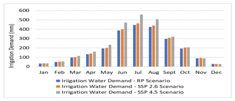
Figure 9. The projected irrigation water demand of the Tharthar Reservoir
Figure 10. The projected municipal water demand of the Tharthar Reservoir
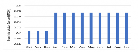
Figure 11. The projected industrial water demand of the Tharthar Reservoir
2. Projection of the inflow of the reservoir: The wet and dry year criteria can be adopted as a scenario for the operation reservoir for the planning period from October 2022 to September 2059. The years within this period will be classified as two wet years and two dry years based on this scenario. Figure 8 shows the average monthly inflow of the Tharthar Reservoir in dry and wet years, respectively.
3. Projection of the water demand: Figure 9 shows the mean value of the irrigation water requirement for the three climate scenarios RP, SSP1-2.6, and SSP2-4.5. The total irrigation water was estimated by summation of the demand of the Babil and Diwaniyah provinces. The actual capacity of WTPs and CU data can be divided by the resident number for the Babil and Diwaniyah provinces to project the monthly water demand for the municipal sector. This criterion can be adopted to derive the water demand per capita from October 2022 to September 2059.
Figure 10 shows the projected municipal water demand of the Tharthar Reservoir. The data shown in Table 5 can be adopted for generating the industrial demand data from 2022 to 2060. Figure 11 shows the projected municipal water demand of the Tharthar Reservoir.
3.2 The optimal outflow and rule curves of the storage
Two cases after running the model can apply to the Tharthar Reservoir; case A: If scenario TH1 implementing in the optimal operation of the Tharthar Reservoir, the plan is unsafe during the planning period of the operation from October 2022 to September 2059 because there is a deficit in the storage and outflow. The summation losses of the deficit in the storage and outflow are 52671 (MCM). The reasons for the deficit in the storage and outflow are the high evaporation from the surface area of the Tharthar Reservoir, low precipitation, high irrigation and municipal requirements consumption, and low inflow to the reservoir. Case B: The alternative scenario TH2 can be adopted because the losses in storage and outflow are smaller than in Case A. The summation losses of the deficit in the storage and outflow are 13071 MCM. The reduction in the losses of the storage and outflow after applying case B is 75%. The alternative scenario TH2 can decrease the deficit in release for operating the Tharthar Reservoir. Figure 12 shows the optimal outflow for Tharthar Reservoir. From Figure 12 can be noticed that the jump in the values of the projected outflow increased rapidly after 2039, because of the increase in the demand for water due to the high temperature, low rainfall, and decreasing humidity, according to the climate change scenario SSP2-4.5, and the increasing in evaporation rate and water consumption for the agricultural and Municipal sectors. Figure 13 shows the monthly optimal outflow for the operating reservoir.
Figure 12. The time series of the optimal outflow for Tharthar Reservoir
Figure 13. The average monthly of the projected optimal outflow for cases A and B
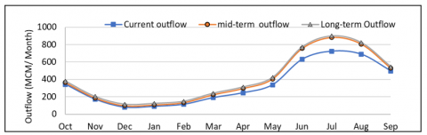
Figure 14 compares the reservoir's current, mid-term, and long-term outflow. There is an increase in the outflow for the mid-term and long-term concerning the current year, equaling 16.4 and 18%. The operating policies consist of the maximum and minimum of the annual outflow. The maximum value of the policies cases A and B represents the water year 2058, where the total annual of the optimal policies is equal to 4983 MCM, and the minimum value is 2022, where the total annual of the optimal policies is equal to 4110 MCM. The operation rule curves of the Tharthar Reservoir can be derived from the optimization model results. The rule curve represents the average monthly optimum storage period from October 2022 to September 2059. From the results of the optimal water storage after running the model in which the scenario TH2 is the solution to the problem of the storage deficit for the Tharthar Reservoir. Figure 15 shows the rule curve of the optimum storage for the Tharthar Reservoir. The maximum storage is equal to 60901 MCM in May. The minimum storage is equal to 1747 MCM in December. The upper and lower rule curves behave the same as the average rule curve, but the lower rule curve converges to the minimum storage except from October to February. The maximum and minimum average of the operational storage was equal to 35825 MCM in May and 31065 MCM in October. The storage increases from January to peak storage in May and, after this point, decreases gradually until it reaches minimum storage in September. The rule curve based on the optimum WSE can be derived from Eqs. (29)-(31). Figure 16 shows the maximum operational WSE where equal to 38.72 (m.a.s.l) in May. The minimum operational WSE was equal to 33.45 (m.a.s.l) in December.
Figure 14. The optimal outflow of the short, mid-term and long-term
Figure 15. The rule curves of the optimum storage of the TH2 scenario
Figure 16. The rule curve is based on the optimum WSE of the TH2 scenario
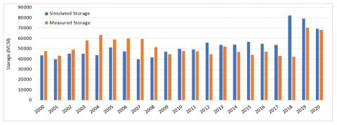
Figure 17. The comparison between simulated and measured storage
Figure 18. The comparison between the simulated outflow by DDDP and WEAP mode
3.3 Verification of the storage and outflow results
Optimization model reliability depends upon the verification of the results. For Tharthar Reservoir can be implemented the data measured from 2000 to 2020. The values of the coefficient of determination (R2), NSE, and RSR are equal to 0.71, 0.68, and 0.57, respectively. Figure 17 shows the correlation between the simulated and measured storage. Generally, the verification processes applied to the results of the two models, DDDP and WEAP. The supply recorded good accuracy for the simulation times. The optimal values of the three statistical parameters R2, NSE, and RSR were viewed as an acceptable level of DDDP and WEAP Model for Tharthar Reservoir. The value of the coefficient of determination R2, NSE, and RSR are equal to 0.95,0.94, and 0.24 for the Tharthar Reservoir, respectively. Figure 18 shows the comparison between the calculated outflow by DDDP and WEAP model.
All the following results represent the outputs of the optimization model during the planning duration from October 2022 to September 2059. The cumulative water inflow to the Tharthar Reservoir equals 301209 MCM, and the evaporation rate from the reservoir equals 193546 MCM. The cumulative water demand is equal to 168929 MCM. The mid-and long-term release increases concerning the current year equal 16.4 and 18%, respectively. The reasons for this increase are urban, agricultural, and industrial expansion and climate change's impact. The three statistical parameters, R2, NSE, and RSR, were evaluated as an acceptable level and a good agreement of the performance from verifying the simulated and measured storage. Also, the comparison between the outflow of the DDDP model and the WEAP model. At the end of the planning period, the reservoir's storage will equal 4445 MCM. The municipal and industrial sectors should prioritize the water supply for the governorates within the ERB and feed from the reservoir. Finally, the strategy is safe if the scenario TH2 scenario is applied to the optimal operation by using the optimization model.
[1] Loucks, D.P., Van Beek, E. (2017). Water resources planning and management: an overview. Water Resource Systems Planning and Management, 1-49. https://doi.org/10.1007/978-3-319-44234-1_1
[2] United nations economic and social commission for western Asia. (2013). Inventory of Shared Water Resources in Western Asia, Beirut.
[3] Al-Ansari, N. (2013). Management of water resources in Iraq: perspectives and prognoses. Engineering, 5(8): 667-684. https://doi.org/10.4236/eng.2013.58080
[4] Al-Ansari, N., Adamo, N., Sissakian, V.K., Knutsson, S., Laue, J. (2018). Water resources of the Euphrates river catchment. Journal of Earth Sciences and Geotechnical Engineering, 8(3): 1-20.
[5] Chow V.T., Cortes-Rivera G, (1974). Application of DDDP in water resources planning. University of Illinois at Urbana-Champaign, Water Resources Center.
[6] Murray, D.M., Yakowitz, S.J. (1979). Constrained differential dynamic programming and its application to multireservoir control. Water Resources Research, 15(5): 1017-1027. https://doi.org/10.1029/WR015i005p01017
[7] Murray, D.M., Yakowitz, S.J. (1984). Differential dynamic programming and newton's method for discrete optimal control problems. Journal of Optimization Theory and Applications, 43(3): 395-414. https://doi.org/10.1007/BF00934463
[8] Al-Delewy, A.H., Ali, A.A., Motalib, R.H. (2005). Optimum operation of Makhool dam. Journal of Engineering and Development, 9(1).
[9] Mohammed, R.K. (2010). Optimum operation of Haditha dam. Engineering & Technology Journal, 28(24): 7058-7068.
[10] Al-Mansori, N.J., (2017). The optimal operation of Haditha Reservoir by Discrete Differential Dynamic Programming (DDDP). Journal of Babylon University/Engineering Sciences, 25(4): 1206-1211.
[11] Ali, A.A.S.M., Abed, Z.H. (2018). Derivation of operation rule for Ilisu dam. Journal of Engineering, 24(6): 53-71. https://doi.org/10.31026/j.eng.2018.06.05
[12] Avarideh, F., Attari, J., Moridi, A. (2017). Modelling equitable and reasonable water sharing in transboundary rivers: the case of Sirwan-Diyala river. Water Resources Management, 31: 1191-1207. https://doi.org/10.1007/s11269-017-1570-4
[13] AlMohseen, K.A., Klari, Z.M. (2016). Effect of Bekhma reservoir system on the water management plan for selected area in greater zab river basin. ZANCO Journal of Pure and Applied Sciences, 28(2): S264-269.
[14] Sameer, S.M., Mustafa, A.S., Al-Somaydaii, J.A. (2021). Study of the sustainable water resources management at the upper Euphrates Basin, Iraq. International Journal of Design & Nature and Ecodynamics, 16(2): 203-210. https://doi.org/10.18280/ijdne.160210
[15] Noon, A.M., Ahmed, H.G., Sulaiman, S.O. (2021). Assessment of water demand in Al-Anbar Province-Iraq. Environment and Ecology Research, 9(2): 64-75. https://doi.org/10.13189/eer.2021.090203
[16] Al-Mukhtar, M., Mutar, S. (2021). Modelling of future water use scenarios using WEAP model: A case study in Baghdad city, Iraq. Engineering and Technology Journal, 39(3): 488-503. https://doi.org/10.30684/etj.v39i3A.1890
[17] Sharef, A.J., Dara, R.N., Ahmed, A.R. (2021). Greater Zab River basin planning (2050). Iraqi Journal of Agricultural Sciences, 52(5): 1150-1162. https://doi.org/10.36103/ijas.v52i5.1453
[18] Sissakian, V.K. (2011). Genesis and age estimation of the Tharthar depression, central West Iraq. Iraqi Bulletin of Geology and Mining, 7(3): 47-62.
[19] Abdullah, M., Al-Ansari, N., Laue, J. (2019). Water resources projects in Iraq: Reservoirs in the natural depressions. Journal of Earth Sciences and Geotechnical Engineering, 9(4): 137-152.
[20] JICA (2016). Data collection survey on water resource management and agriculture irrigation in the republic of Iraq final report. Japan International Cooperation Agency (JICA). NTC International Co., Ltd.
[21] Al-Khuzaie, M.M., Abdul Maulud, K.N., Mohd Taib, A. (2022). Soil salinity monitoring and quantification using modern techniques. Journal of Ecological Engineering, 23(11): 57-67. https://doi.org/10.12911/22998993/152542
[22] Labadie, J.W. (2004). Optimal operation of multireservoir systems: State-of-the-art review. Journal of Water Resources Planning and Management, 130(2): 93-111. https://doi.org/10.1061/(ASCE)0733-9496(2004)130:2(93)
[23] Goor, Q., (2010). Optimal operation of multiple reservoirs in hydropower-irrigation systems: A stochastic dual dynamic programming approach. PhD thesis in Environmental Sciences, Earth and Life Institute, Catholic University of Louvain, Belgium.
[24] Heidari, M., Chow, V.T., Kokotović, P.V., Meredith, D.D. (1971). Discrete differential dynamic programing approach to water resources systems optimization. Water Resources Research, 7(2): 273-282. https://doi.org/10.1029/WR007i002p00273
[25] Goor, Q., Kelman, R., Tilmant, A. (2011). Optimal multipurpose-multireservoir operation model with variable productivity of hydropower plants. Journal of Water Resources Planning and Management, 137(3): 258-267. https://doi.org/10.1061/(ASCE)WR.1943-5452.0000117
[26] Allen, R.G., Smith, M., Pereira, L.S., Raes, D., Wright, J.L. (2000). Revised FAO procedures for calculating evapotranspiration: irrigation and drainage paper no. 56 with testing in Idaho. In Watershed Management and Operations Management, 2000: 1-10. https://doi.org/10.1061/40499(2000)125
[27] Naidu, C.R., Giridhar, M.V.S.S. (2015). Irrigation demand VS supply-remote sensing and GIS approach. Journal of Geoscience and Environment Protection, 4(1): 43-49. https://doi.org/10.4236/GEP.2016.41005
[28] United Nations (2019). World population prospects 2019, volume i: Comprehensive tables. New York: Population Division, Department of Economic and Social Affairs, United Nations.
[29] RIMP, (2013). Republic of Iraq Ministry of Planning National Development Plan 2013-2017, Baghdad.
[30] Aljanabi, A.A.A. (2019). Optimization models for Iraq's water allocation system. Doctoral dissertation, Arizona State University.
[31] SWLRI. Iraqi Ministry of Water Resources. Strategy for Water and Land Resources in Iraq. Ministry of Water Resources. https://t-zero.it/en/portfolio/swlri-strategy-for-water-and-land-resources-in-iraq/, accessed on Oct. 06, 2015.
[32] WHO, H. (2011). World health organization guidelines for drinking-water quality. World Health Organization.
[33] NCFWRM. (2022). National Center for Water Recourses Management in Iraq. Unpublished data.
[34] Moriasi, D.N., Arnold, J.G., Van Liew, M.W., Bingner, R.L., Harmel, R.D., Veith, T.L. (2007). Model evaluation guidelines for systematic quantification of accuracy in watershed simulations. Transactions of the ASABE, 50(3): 885-900. https://doi.org/10.13031/2013.23153
[35] KhazaiPoul, A., Moridi, A., Yazdi, J. (2019). Multi-objective optimization for interactive reservoir-irrigation planning considering environmental issues by using parallel processes technique. Water Resources Management, 33: 5137-5151. https://doi.org/10.1007/s11269-019-02420-7
[36] Chu, T.W., Shirmohammadi, A., Montas, H., Sadeghi, A. (2004). Evaluation of the swat model’s sediment and nutrient components in the piedmont physiographic region of Maryland. Transactions of the ASAE, 47(5): 1523-1538. https://doi.org/10.13031/2013.17632
[37] Boyle, D.P., Gupta, H.V., Sorooshian, S. (2000). Toward improved calibration of hydrologic models: Combining the strengths of manual and automatic methods. Water Resources Research, 36(12): 3663-3674. https://doi.org/10.1029/2000WR900207
[38] Legates, D.R., McCabe Jr, G.J. (1999). Evaluating the use of “goodness‐of‐fit” measures in hydrologic and hydroclimatic model validation. Water resources research, 35(1): 233-241. https://doi.org/10.1029/1998wr900018