Son Tung Dang![]() | Hai Anh Nguyen*
| Hai Anh Nguyen*![]() | Hai Duong Nguyen | Tran Thi Minh Kieu
| Hai Duong Nguyen | Tran Thi Minh Kieu
© 2023 IIETA. This article is published by IIETA and is licensed under the CC BY 4.0 license (http://creativecommons.org/licenses/by/4.0/).
OPEN ACCESS
In this paper, we will present a numerical framework to simulate the weapon operation for air-to-air missiles (AAM) on the super manoeuvrable fighter aircraft (Flanker C). We focus on creating a flexible and robust framework to insert into any flight simulator for training pilots to operate the air-to-air missile system. In general, the framework contains four main parts: (1) virtual target; (2) avionics systems; (3) head-up display system; (4) missile flight dynamics. The results of both semi-active radar and infrared homing missiles show the flexibility and robustness of the proposed framework in simulating the weapon operation.
weapon operation simulation, modelling and simulation, avionics system, air-to-air missiles
The fighter jet simulation, nowadays, becomes more prevalent due to the fact that it will reduce the cost for training pilots. In addition, the simulation will be able to create various test cases, which rarely occur in the actual combat. Several computer-based flights have been developed in recent years to simulate aircraft aerodynamics such as the F-22 simulator [1]. The weapon system is an important and complicated unit of the jet fighter such that it decides the outcome of air combat. Therefore, simulation is a suitable and economical method for training pilots and enhancing the operational ability of weapon system, which are missiles and avionic units. There are several methods to compute the missile trajectory. The first method employs 3DOF equations of motion [2], which ignores all rotational motion of the missile. In comparison with the 6DOF equations, the application of the 3DOF formulas is less time-consuming, although the result is less accurate when the missile operates in a low altitude. The 6DOF equations [3-5] are applied to predict the missile trajectory for both aerial and ground targets. In complex simulation scenarios, which involve multi-object simulations, the most important factor is the computing time. All equations have to be solved as fast as possible such that results are available for visualization process. Especially, for smooth dynamic motion, the frame rate can be up to 120 Hz. Therefore, in this study, we will present a method to calculate the missile trajectory, which will ensure the missile hit the target. For avionic systems, which are electrom/agnetic radar and infrared search and track system (IRTS), we will assume that systems will always detect targets inside their effective range except for particular cases. This assumption is needed to re-create a good working condition system for training purposes. It is meaningful for students when they make manipulations and observe, evaluate the results. In addition, this will reduce the complexity of radar simulation, which requires solving the wave transform equation [6], five warnings scattering and absorption [7], and the cross-section of object [8]. As a result, the time needed for spotting targets on HUD will be small enough that the weapon system operator can lock on targets quickly.
The objective of research is to propose a mathematical framework simulating an air-to-air missile operation on fighter aircraft, in which, the missile trajectory and avionics systems are modelled for training purposes (ideal working condition, high performances and sufficient functions). The framework is designed to be robust and able to simulate various missile models. Major novelty contributions of the paper are listed as follows:
1. A complete mathematical framework of weapon simulation is proposed and validated for two different types of missiles. Hence, the weapon operation process is fully simulated for training purpose.
2. In the operation process, detecting a target using the radar system is an important step. It is sensitive with type, state of target, and surrounding environment. Therefore, in this work, the characteristic of radar systems is an in-depth analysis, then, re-created in the simulation.
3. A mathematical model is proposed to compute the trajectory of missile. The method will simulate a sequence of missile flight phases which is typical to the air to air missile.
The content of paper consists of three main parts: (1) Introduction section presents an overview and scope of research; (2) Mathematical model will define coordinate systems and give more details about the target simulation, avionics systems, and the missile dynamic equations; (3) Simulation results validated our work for two types of missiles. Finally, Conclusion part briefly summarise our contribution and results of the study.
2.1 Coordinate systems
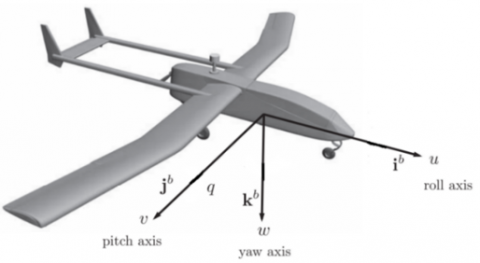
The inertial coordinate (Fi) is a Cartesian earth-fixed frame whose origin is defined at a given location. The coordinate is sometimes referred to as the north-east-down (NED) reference frame. The vehicle coordinate (Fv) is a frame whose origins is defined at the center of mass of the aircraft. Its axes will be aligned with corresponding axes in the inertial frame as in Figure 1. The body coordinate is a frame that sticks to the aircraft as in Figure 2. Therefore, it will rotate following the jet motion. In general, the relation between the inertial and vehicle coordinate is translation. The body frame, on the other hand, is obtained from the vehicle frame by rotation. The rotation matrix that is derived from rotating the vehicle frame to achieve the body frame is given by Beard and McLain [9].
$R_v^b=\left(\begin{array}{ccc}c_\theta c_\psi & c_\theta s_\psi & -s_\theta \\ s_\phi s_\theta c_\psi-c_\theta s_\psi & s_\phi s_\theta s_\psi+c_\phi c_\psi & s_\phi c_\theta \\ c_\phi s_\theta c_\psi+s_\phi s_\psi & c_\phi s_\theta s_\psi-s_\phi c_\psi & c_\phi c_\theta\end{array}\right)$ (1)
where, cϕ = cos(ϕ) and sϕ = sin(ϕ). ϕ, θ, and ψ are Euler angles, which are also referred as roll, pitch, and yaw respectively as in Figure 3. The rotation matrix from the body frame to the vehicle frame is given by
$R_b^v=\left(R_v^b\right)^T=\left(\begin{array}{ccc}c_\theta c_\psi & s_\phi s_\theta c_\psi-c_\theta s_\psi & c_\phi s_\theta c_\psi+s_\phi s_\psi \\ c_\theta s_\psi & s_\phi s_\theta s_\psi+c_\phi c_\psi & c_\phi s_\theta s_\psi-s_\phi c_\psi \\ -s_\theta & s_\phi c_\theta & c_\phi c_\theta\end{array}\right)$ (2)
Figure 1. The definition of initial and vehicle frame [9]
Figure 2. The definition of the body frame [9]
Figure 3. The definition of roll ($\phi$), pitch ($\theta$), and yaw ($\psi$) angles and how to obtain the body frame from the vehicle frame [9]
The translation matrix from the vehicle frame to the inertial frame is obtained as follows:
$T_v^i=\left(\begin{array}{cccc}1 & 0 & 0 & x_v^i \\ 0 & 1 & 0 & y_v^i \\ 0 & 0 & 1 & z_v^i \\ 0 & 0 & 0 & 1\end{array}\right)$ (3)
where, $x_v, y_v$, and $z_v$ are the location of vehicle’s origin in the inertial frame. The position of an object converted from the body frame to the inertial frame is obtained by
$\left(\begin{array}{c}x^i \\ y^i \\ z^i \\ 1\end{array}\right)=M_b^i\left(\begin{array}{c}x^b \\ y^b \\ z^b \\ 1\end{array}\right)$ (4)
where, $x^i, y^i$, and $z^i$ are the location of a target in the inertial frame while $x^b, y^b$, and $z^b$ and are its value in the body frame. The complete transform matrix $M_b^i$ are computed by
2.2 Target simulation
Target simulation is an important task of the proposed framework. The main goal of this task is to re-create the action of the target following the demand of training. In general, target simulation which is presented in Figure 4, focus on three main aspects: (1) target type, (2) target behaviours [10, 11], and (3) flight dynamics referring to the study [12]. The target type defines the characteristic of target, the dynamical features and the corresponding set of actions. Target behaviours are the set of predefined actions for airborne target, which is classified by the level of task difficulty. In a given scenario, and at the same level of task difficulty, the behaviour of the target is defined by the conditional selection sets of action. In this work, 30 actions and 05 levels are implemented to simulate the common behaviours of the target. For example, steady moving is the simplest action at the lowest level. Kulbit [13] is the most complicated action at the highest level. Target flight dynamics solves a set of derivative equations to calculate the trajectory of target.
Figure 4. Target simulation diagram
2.3 Avionic systems
2.3.1 Phased array radar
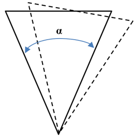
In the fighter aircraft, the phased bar array radar is used to detect targets. Then, targets will be depicted on the HUD to indicate that they are found by the radar as shown in Figure 5. In this study, we simplify the principles of phased bar array radar such that we can reduce the complexity of mathematical modelling, and the computational time. Figure 6 represents the radar beam. Flying objects are detected if their position is inside, and their relative distance to the radar is smaller than the maximum detection range. In our work, the opening azimuth (α) and elevation angle (β) are 60º and 30º respectively. Several 2D coordinate systems are used to compute the position of targets on the HUD. The first coordinate system is azimuth-radial distance, where the width of HUD is aligned with the azimuth axis varying from -30º to 30º, and the height is aligned with the radial distance axis ranging from 0 to 100km. This coordinate is usually applied for targets moving in the opposite direction to the jet motion. The second coordinate system is azimuth-velocity, in which the height of HUD represents the relative velocity between the jet and the target. It will be employed when targets and jet fly in the same direction. Because it is more difficult for electromagnetic radar to spot objects when the relative velocity between the aircraft and targets are small, in this paper, we will focus on the azimuth-radial distance. Giving the position of the target ($x_t^i, y_t^i, z_t^i$) and the jet ($x_j^i, y_j^i, z_j^i$) in the inertial frame, the location of target ($x_t^b, y_t^b, z_t^b$) in the body frame is computed as follows:
$\left(\begin{array}{c}x_t^b \\ y_t^b \\ z_t^b \\ 1\end{array}\right)=M_i^b\left(\begin{array}{c}x_t^i \\ y_t^i \\ z_t^i \\ 1\end{array}\right)$ (6)
where, the transform matrix ($M_b^i$) is computed by
$M_i^b=\left(M_b^i\right)^{-1}$ (7)
with is determined from Eq. 5. The azimuthal angle of the target in the body frame is estimated by
$\theta_t^b=\tan ^{-1} \frac{y_t^b}{x_t^b}$ (8)
In order to search in other region in air space, the radar can change the direction as shown in Figure 7. The radar beam can move in both elevation and azimuth plane following the elevation and azimuth coverage bar as in Figure 5. In this study, the azimuth varies from -30º to 30º while the elevation angle range is from -7.5º to 15.0º. Assume that we switch the radar heading direction to -30º on the left as in Figure 5, the new azimuthal angle of target is computed by
$\theta_t^{b, n e w}=\tan ^{-1} \frac{y_t^b}{x_t^b}+30^{\circ}$ (9)
As a result, the target will appear on the right side of HUD if $\theta_t^{b,new}$ is still inside the radar beam.
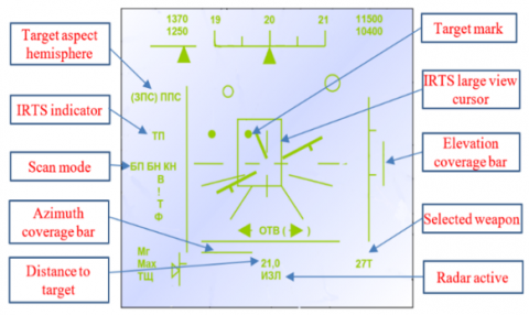
Figure 5. The HUD displays the seeking mode with phased array radar, which can operate in several scan modes. If the anonymous flying objects are inside the detected region that is bounded by elevation, azimuth coverage, and expected target range they will be spotted on HUD screen. The target is selected by moving the radar cursor over identified flying object, and then pressing a lock button [14]
Figure 6. The radar beam in which targets can be tracked down. α is opening azimuth, β is opening elevation angle
(a) Change the radar beam heading in the elevation plane
(b) Change the radar beam heading in the azimuth plane
Figure 7. Moving radar direction to change the detection region of radar
2.3.2 Infrared search and track system
Infrared search and track system (IRTS) is a technique for detecting and tracking anonymous objects, which generate infrared radiation as shown in Figures 8 and 9. The IRTS is usually employed when the target transport in the same direction as the jet, because the target’s engine is the main thermal source pointing directly to the jet front. The IRTS will operate in the seeking mode first to depict anonymous flying objects on HUD as represented in Figure 8. Figure 9 shows the identification mode after the seeking mode determine the region where the target is possibly located. The IRTS cannot provide information about the distance between an object and the jet. Therefore, in this work, object positions are computed in the elevation angle-azimuth coordinates to indicate the direction from the jet to an infrared radiation source. The elevation angle can be computed by
$\phi=\tan ^{-1} \frac{-y_t^b}{\sqrt{\left(x_t^b\right)^2+\left(y_t^b\right)^2+\left(z_t^b\right)^2}}$ (10)
where, ($x_t^b, y_t^b, z_t^b$) is location of target in the body frame, which is computed from Eq. 6. The HUD height will coincide with the elevation angle varying from -30º to 30º, while the HUD width will align with azimuth ranging from -30º to 30º. The size of large view cursor is 20º width x 30º height. After moving the cursor to the region containing the suspected target, a button is released to change HUD screen to small view mode such that targets can be distinguished from the other objects. In this mode, the dimension of HUD will coincide with the size of large view cursor depicted in Figure 8. The size of small view cursor in Figure 9 is 7º width x 15º height. In this mode, the target will be locked, then, its location will be used for guiding missile.
Figure 8. The HUD displays the large view mode with infrared search and track system, where flying objects are detected due to their thermal radiation. They are spotted on HUD screen by target marks. The IRTS large view cursor will move around HUD looking for potential targets. After the suspected target is determined, the large view mode will change to small view mode [14]
Figure 9. The HUD displays the small view mode with infrared search and track system. In this mode, the target is determined by moving the IRTS mall view cursor over identified flying object, and then pressing a lock button [14]
2.4 Missile dynamic
After the target is locked-on, the pilot will decide to launch the missile when the threat inside the missile range. There are two modes in the missile operation. At first, the missile will slide on the launching rail until it detaches entirely from the jet. Then, the missile will change its direction such that it will follow and destroy the target. The equation describing the motion of missile is given as follows:
$m \boldsymbol{a}_m=\boldsymbol{F}_{\text {thrust }}-\boldsymbol{F}_D$ (11)
where, $\boldsymbol{F}_{\text {thrust }}$ is thrust force produced by missile engine, $\boldsymbol{F}_D$ is the drag force, which can computed by
$F_D=C_D \frac{\rho_{a i r} \,\, v^2}{2} A$ (12)
where, ρair is air density, $C_D$ is the drag coefficient, v is the missile velocity vector, and A is the missile reference area, which is evaluated by
$A=\pi \frac{D^2}{4}$ (13)
where, D is the missile diameter. In this paper, we ignore the lift force and gravity. We only focus on the thrust and drag forces, which are the main forces contributing to the missile acceleration. The missile operation consists of two phases. The first phase is a sliding mode, in which the missile slide on the trailing rail. In this case, the missile steers the same direction as the jet motion. After the missile complete sliding on the trail, the second phase takes place. In this phase, the missile head directly to the target. The position of the missile in the inertial frame ($x_m^i, y_m^i, z_m^i$) can be computed from its location in the body frame ($x_m^b, y_m^b, z_m^b$) by
$\left(\begin{array}{c}x_m^i \\ y_m^i \\ z_m^i \\ 1\end{array}\right)=M_b^i\left(\begin{array}{c}x_m^b \\ y_m^b \\ z_m^b \\ 1\end{array}\right)$ (14)
The velocity of missile in the body frame ($u_m^b, v_m^b, w_m^b$) is determined in the inertial frame ($u_m^i, v_m^i, w_m^i$) as follows:
$\left(\begin{array}{c}u_m^i \\ v_m^i \\ w_m^i \\ 0\end{array}\right)=M_b^i\left(\begin{array}{c}u_m^b \\ v_m^b \\ w_m^b \\ 0\end{array}\right)$ (15)
2.4.1 Sliding mode
In this mode, the missile will slide on the rail. Before the missile is launched, its initial velocity is identical to the jet velocity. The missile velocity in the roll axis $u_m^b$ is updated by
$u_m^{b, n+1}=u_m^{b, n}+a_m^{b, n} \Delta t$ (16)
where, $n+1$ and $n$ represent the time step, $a_m^{b, n}$ is the missile acceleration, and $\Delta t$ is a time step size. In this study, the time step size 0.01 is used. The relative distance $L$ between the missile and the jet in the roll axis is computed by
$L^{n+1}=L^n+\Delta L^{n+1}$ (17)
where, $\Delta L$ is a distance the missile moved in $\Delta t$. The variable is computed by
$\Delta L^{n+1}=\left(u_m^{b, n}-u_j^{b, n}\right) \Delta t+\frac{1}{2} a_m^{b, n} \Delta t^2$ (18)
The position of missile is updated in the body frame by
$\begin{gathered}x_m^{b, n+1}=x_j^{b, n+1}+L^{n+1} \\ y_m^{b, n+1}=y_j^{b, n+1} \\ z_m^{b, n+1}=z_j^{b, n+1}\end{gathered}$ (19)
Inserting Eq. 19 into Eq. 14, the position of the missile in the inertial frame can be computed accordingly. This mode is terminated when the relative distance L exceeds the rail length. Then, the missile will switch to a target heading mode.
2.4.2 Target heading mode
In this mode, the target position will be used to modify the shift distance, which the missile transport in a time step size $\Delta t$. This mode will mimic the principle of radar guidance. The equation to compute the missile position is given by
$\frac{d^2 x}{d t^2}=a_m$ (20)
In this stage, the missile will head toward the target and change direction following target motion.
$\begin{aligned} & \Delta x_m^{n+1}=u_m^n \Delta t+\frac{1}{2} a_{m, x}^n \Delta t^2 \\ & \Delta y_m^{n+1}=v_m^n \Delta t+\frac{1}{2} a_{m, y}^n \Delta t^2 \\ & \Delta z_m^{n+1}=w_m^n \Delta t+\frac{1}{2} a_{m, z}^n \Delta t^2\end{aligned}$ (21)
The Rodriquez rotation [15] is employed to re-compute the distance that the missile flew in $\Delta t$. It will rotate to the direction from the previous missile position to the most updated target location as in Figure 10. Set $k_{m, t}$ is the vector connecting the target and the missile, $\Delta s^{n+1}\left(\Delta x_m^{n+1}, \Delta y_m^{n+1}, \Delta z_m^{n+1}\right)$ is shifting vector. The new distance is computed based on Rodriquez rotation as follows:
$\begin{gathered}\Delta s_{\text {rot }}^{n+1}=\Delta s^{n+1} \cos \alpha+\left(\boldsymbol{k} \times \Delta s^{n+1}\right) \sin \alpha \\ +\boldsymbol{k}\left(\boldsymbol{k} \cdot \Delta s^{n+1}\right)(1-\cos \alpha)\end{gathered}$ (22)
where, $\boldsymbol{k}$ is determined by
$\boldsymbol{k}=\Delta s \times v_{m j}$ (23)
where, $v_{m j}$ is the vector connecting the missile and jet position at the time step n and n + 1 respectively. Then, the new position of missile can be updated by
$\begin{aligned} & x_m^{n+1}=x_m^n+\Delta x_{\text {rot }}^{n+1} \\ & y_m^{n+1}=y_m^n+\Delta y_{\text {rot }}^{n+1} \\ & z_m^{n+1}=z_m^n+\Delta z_{\text {rot }}^{n+1}\end{aligned}$ (24)
Figure 10. Redirect the missile such that it keeps heading to the target
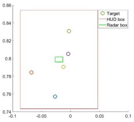
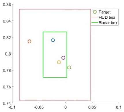
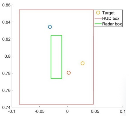
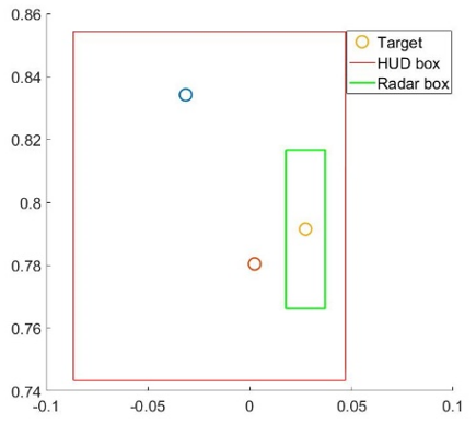
Figure 11 depicts the representation of targets on the HUD screen as they are detected by electromagnetic radar. Table 1 shows the initial position of the jet and five Anonymous Flying Vehicles (AFVs) in the inertial frame for testing the phased array radar. In order to detect targets, there are several researches [16, 17] in literature employ novel signal processing method. However, this method is rather complicated to implement in simulation platform [18, 19], which require fast and robust computation. Therefore, our method, which apply simplistic principles will be suitable for such platforms. Figure 11 illustrates the AFVs position in the HUD screen. In this paper, the maximum detected range is approximately 150000 m. The open-angle of radar varies from -30o to 30o in the wing direction, which is from the left to the right. It can be seen that the position of AFVs in the HUD plane varies depending on the relative location of targets and the jet. All 5 AFVs are detected by the radar as their locations are inside the effective range of the radar. Figure 12 shows the target selection procedure. At first, the radar box will move to the region where the target locates. Then, a button is released to lock-on target. If there are several enemy airborne targets in the same region, the target, which is closest to the box’s centre will be chosen. After the target is selected, its position will be used in the missile dynamic computation to mimic the phenomenon that the missile is guided by the radar system. The initial position of jet and AFVs in the inertial frame, which is used for validating the infrared search and track system, are given in the Table 2. The AFVs in this case will be closer to the jet compared to the radar test case. The HUD display will be in the seeking mode as presented in Figure 13. Several works [20, 21] have proposed a complex method, which require additional information about environment temperature and IRTS sensor. However, this data is not always available due to lacking of reference source and massive data storage requirements. Simulators such as Unity [18] or VBS3 [19] provide features to add models and create a virtual environment. However, there is no option to insert the thermal data into specific regions in the virtual environment. Therefore, our method which does not require additional information about our surroundings is easily implemented in these platforms. In this mode, the box will move around to select the region that might contain the target. After choosing the region at the centre of HUD, the system will change to identification mode, which is shown in Figure 14. The position of AFVs on the HUD, in this case, is their relative positions in the large box in Figure 13. Only three of five AFVs are depicted on the HUD as they are inside the box in the seeking mode. The remaining AFVs are not displayed as they are outside the box. By moving the radar box around the HUD, the target will be selected if its location is closest to the radar box’s centre as in Figure 15. Similar to the radar system, after the IRTS determined the target, its location will be used for guiding the missile to destroy the threat. The missile dynamics is applied to compute the missile trajectory after the target is chosen. In this paper, the missile mass is 230 kg. The engine thrust is set up at 9900 N. The length of missile is 4.08 m while its diameter is 0.23 m. Firstly, the test where the jet and the target move in the opposite direction is performed to validate our method. In this test, the initial value of acceleration, velocity, and position for the jet and target are provided in Table 3. Their x-component of the velocity have a different sign as they travel in the confrontational direction. In this case, the semi-active radar homing missile is deployed. And it will be activated by using the phased array radar to lock-on the target.
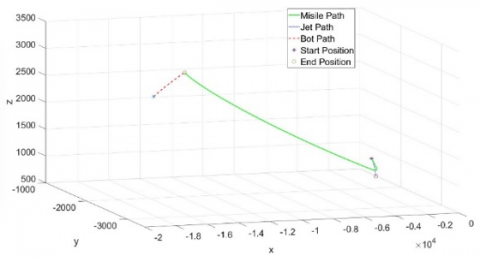
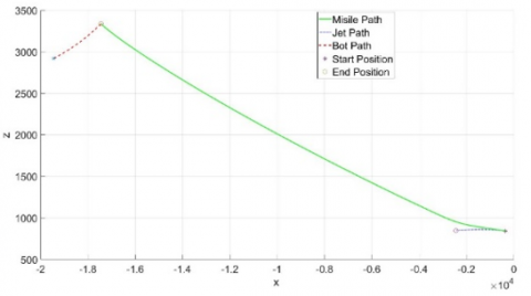
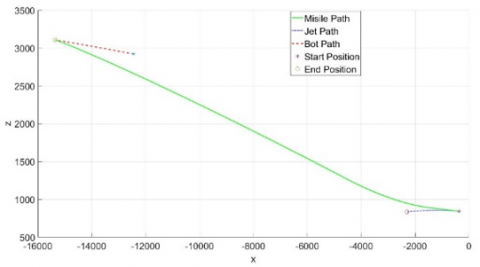
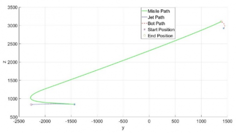
Figure 16 shows the computed missile trajectory as well as the jet and target path in 3D view, in the x-z, and y-z planes respectively. The missile is launched at t = 0, then it moved in the same direction of jet motion, as the missile slides on the launching trail. After that, it will slightly change the heading direction such that it will hit the target eventually as represented in Figure 16. Table 4 provides the initial condition for the jet and target when the infrared homing missile is used. Because the jet and the enemy aircraft move in the same direction, the target engine, which is the main heat source is placed ahead of the missile. The IRTS is deployed for tracking the target. Figure 17 depicted the missile trajectory in 3D view, in the x-y, and y-z planes. In general, the missile path is similar to the previous test, although it requires slightly more time to reach the target.
Table 1. The initial states of jet and target for testing the phased array radar
|
|
Initial Position |
|
jet |
6370 m, -1430 m, -5043 m |
|
aerial vehicle 1 |
13970 m, -2450 m, -5277 m |
|
aerial vehicle 2 |
57670 m, -21590 m, -5395 m |
|
aerial vehicle 3 |
69970 m, 2260 m, -4812 m |
|
aerial vehicle 4 |
89170 m, 8830 m, -4922 m |
|
aerial vehicle 5 |
123370 m, 14290 m, -4611 m |
Table 2. The initial states of jet and target for testing the IRTS system
|
|
Initial Position |
|
jet |
6370 m, -1430 m, -5043 m |
|
aerial vehicle 1 |
17570 m, -1770 m, -5979 m |
|
aerial vehicle 2 |
22470 m, -8150 m, -6451 m |
|
aerial vehicle 3 |
27570 m, -200 m, -4119 m |
|
aerial vehicle 4 |
33970 m, 1990 m, -4559 m |
|
aerial vehicle 5 |
40370 m, 5810 m, -2515 m |
Table 3. The initial states of jet and target for the front approach
|
|
Initial Velocity |
Initial Position |
Initial Acceleration |
|
jet |
-154 m/s, -72 m/s, -6 m/s |
-370 m, -1430 m, -843 m |
-5.2 m/s2, -1.4 m/s2, 1.0 m/s2 |
|
target |
200 m/s, 20 m/s, -30 m/s |
-19443 m, -3435 m, -2920 m |
-4.3 m/s2, -3.4 m/s2, -1.2 m/s2 |
Table 4. The initial states of jet and target for the back approach
|
|
Initial Velocity |
Initial Position |
Initial Acceleration |
|
jet |
-135 m/s, -64 m/s, 5 m/s |
-370 m, -1430 m, -843 m |
-5.2 m/s2, -1.4 m/s2, 1.0 m/s2 |
|
target |
-220 m/s, 10 m/s, -15 m/s |
-12443 m, -3435 m, -2920 m |
-5.3 m/s2, -2.4 m/s2, -0.2 m/s2 |
Figure 11. Electromagnetic radar box and targets depict on the HUD screen
Figure 12. The target is locked on the HUD screen
Figure 13. IRTS in the searching mode and targets depict on the HUD screen
Figure 14. IRTS in the search-to-lock mode on the HUD screen
Figure 15. IRTS system and lock-on target
(a) The missile path in 3D
(b) The missile path in the x-z plane
(c) The missile path in the y-z plane
Figure 16. The missile, jet, and target computed trajectory when the target moves in the opposite direction with the jet
(a) The missile path in 3D
(b) The missile path in the x-z plane
(c) The missile path in the y-z plane
Figure 17. The missile, jet, and target computed trajectory when the target moves in the same direction with the jet
In this paper, we have already presented mathematical methods to simulate air-to-air missile operation on fighter aircraft. Methods are flexible and robust, therefore, they can be applied easily on any simulation system. The computed results show that avionic systems can depict the position of anonymous flying objects in both altitude-azimuth and elevation angle-azimuth coordinates. In addition, the missile dynamics equation can predict the missile path, which leads to the target accurately.
We would like to thank the Modelling and Simulation Centre, Viettel High Technology Industries Corporation for supporting our research.
[1] F-22 Demonstration Simulator. (2020). https://mvrsimulation.com/casestudies/f-22.html.
[2] Brochu, R., Lestage, R. (2003). Three-degree-of-freedom (DOF) missile trajectory simulation model and comparative study with a high fidelity 6DOF mode. DRDC Valcartier TIM, 2003-56.
[3] Wibowo, S.S. (2020). Full envelope six-degree of freedom simulation of tactical missile. AIP Conference Proceedings, 2226(1): 020008. https://doi.org/10.1063/5.0002623
[4] Gkritzapis, D.N., Kaimakamis, G., Siassiakos, K., Chalikias, M. (2008). A review of flight dynamic simulation model of missiles. In 2nd European Computing Conference (ECC’08), pp. 11-13.
[5] Gkritzapis, D.N., Panagiotopoulos, E.E., Margaris, D.P., Papanikas, D.G. (2007). A six degree of freedom trajectory analysis of spin stabilized projectiles. AIP Conference Proceedings, 963(2): 1187-1194. https://doi.org/10.1063/1.2835958
[6] Park, S.H. (2014). Automatic target recognition using jet engine modulation and time-frequency transform. Progress In Electromagnetics Research M, 39: 151-159. https://doi.org/10.2528/PIERM14100701
[7] Srivastava, H.B., Limbu, Y.B., Saran, R., Kumar, A. (2007). Airborne infrared search and track systems. Defence Science Journal, 57(5): 739.
[8] Çakir, G., Sevgi, L. (2010). Radar cross-section (RCS) analysis of high frequency surface wave radar targets. Turkish Journal of Electrical Engineering and Computer Sciences, 18(3): 457-468. https://doi.org/10.3906/elk-0912-7
[9] Beard, R.W., McLain, T.W. (2012). Small Unmanned Aircraft: Theory and Practice. Princeton University Press, USA.
[10] Lam, C.P., Masek, M., Kelly, L., Papasimeon, M., Benke, L. (2019). A simheuristic approach for evolving agent behaviour in the exploration for novel combat tactics. Operations Research Perspectives, 6: 100123. https://doi.org/10.1016/j.orp.2019.100123
[11] Shaw, R.L. (1985). Fighter Combat: Tactics and Maneuvering. Naval Institute Press, Annapolis, MD, USA.
[12] Zhang, R., Zhang, J., Yu, H. (2018). Review of modeling and control in UAV autonomous maneuvering flight. In 2018 IEEE International Conference on Mechatronics and Automation (ICMA), Changchun, China. https://doi.org/10.1109/ICMA.2018.8484542
[13] Joyce, D.A. (2014). Flying Beyond the Stall: The X-31 and the Advent of Supermaneuverability. NASA, USA.
[14] Zhukovsky. (2004). САМОЛЕТ СУ-27СК РУКОВОДСТВО ПО ЛЕТНОЙ ЭКСПЛУАТАЦИИ, Книга 1. JSC KNAAPO, Moscow, Russia.
[15] Liang, K.K. (2018). Efficient conversion from rotating matrix to rotation axis and angle by extending rodrigues’ formula. arXiv preprint, arXiv:1810.02999. https://doi.org/10.48550/arXiv.1810.02999
[16] Lia, Z. (2019). Multi-target CFAR detection of a digital phased array. Journal of Physics: Conference Series, 1314(1): 012011. https://doi.org/10.1088/1742-6596/1314/1/012011
[17] Hu, P., Bao, Q., Chen, Z. (2019). Target detection and localization using non-cooperative frequency agile phased array radar illuminator. IEEE Access, 7: 111277-111286. https://doi.org/10.1109/ACCESS.2019.2934754
[18] Juliani, A., Berges, V.P., Teng, E., Cohen, A., Harper, J., Elion, C., Goy, C., Gao, Y., Henry, H., Mattar, M., Lange, D. (2018). Unity: A general platform for intelligent agents. arXiv preprint, arXiv:1809.02627. https://doi.org/10.48550/arXiv.1809.02627
[19] Fügenschuh, A., Vierhaus, I., Fleischmann, S., Löffler, T., Diefenbach, T., Lechner, U., Knöbel, K., Marahrens, S. (2016). VBS3 as an Analytical Tool-Potentialities, Feasibilities and Limitations. University of the Federal Armed Forces, Hamburg, Germany.
[20] Sozzi, B., Fossati, E., Barani, G., Santini, N., Ondini, A., Colombi, G., Quaranta, C. (2010). Simulator of IRST system with ATR embedded functions. Proc. SPIE 7660, Infrared Technology and Applications XXXVI, 766003. https://doi.org/10.1117/12.849629
[21] Gaitanakis, G.K., Vlastaras, A., Vassos, N., Limnaios, G., Zikidis, K.C. (2019). InfraRed search & track systems as an anti-stealth approach. Journal of Computations & Modelling, 9(1): 33-53.