Sambhaji T Kadam*![]() | Ibrahim Hassan
| Ibrahim Hassan![]() | Liangzhu (Leon) Wang
| Liangzhu (Leon) Wang![]() | Mohammad Azizur Rahman
| Mohammad Azizur Rahman![]()
© 2023 IIETA. This article is published by IIETA and is licensed under the CC BY 4.0 license (http://creativecommons.org/licenses/by/4.0/).
OPEN ACCESS
A correct prediction of building cooling load is essential in building energy consumption in a hot and humid urban area. To this extent, the current study emphasizes a meticulous review of different convective heat transfer coefficient correlations including those developed considering neighbourhood microclimate effect, and the existing ones used in building energy simulation programs such as EnergyPlus, Environmental Systems Performance - Research (ESP-r), Integrated Environmental Solutions Ltd (IES), IDA, and TAS. Furthermore, rigorous quantitative assessment of associated convective thermal load from the windward, leeward, and roof surfaces under the case of microclimatic conditions is performed. The data used in the current assessment are computational fluid dynamics results, as a reference, from previously published data and actual weather data from the hot and humid climate. It is observed that very few convective heat transfer coefficient correlations show closer predicted thermal load (deviation less than 30%) with computational fluid dynamics results, and others exhibit a varying degree of prediction ability with over-predictions in general for the windward, leeward and roof surfaces. Current analysis suggests that further attention is required to increase the prediction ability of convective heat transfer coefficient correlations by developing a convective heat transfer coefficient model considering computational fluid dynamics analysis of the whole district, validating and modifying or redefining existing convective heat transfer coefficient correlations based on real field measurement data considering flow field around the building, and incorporation of urban morphology, vegetation, urban heat island, and urban pollution level in convective heat transfer coefficient correlations development.
convective thermal load, heat transfer coefficient, correlations, BES, microclimate, leeward, windward, roof
The expansion of the building sector to accommodate increasing migrants [1] and support industrial advancement, including commercial and residential, in urban areas leads to substantial use of global energy for space cooling or heating [2, 3]. To achieve the required thermal comfort, it is estimated that 20-50% of energy is consumed by indoor heating, ventilation, and air conditioning (HVAC) systems resulting from the building envelope [4]. Issac and Vuuren [5] estimate that by 2050, global energy usage for air conditioning will be around 15400 PJ, surpassing heating energy use.
Another essential aspect responsible for increasing building energy consumption is climate change, which occurs naturally or by human interventions [6]. These changes are attributed to change in meteorological variables (such as solar radiation, longwave radiation, air temperature, air humidity, air wind speed and direction, and their interactions [7-9]) prevailing over a large area (spatial), usually spanning over several years (temporal). The built environment alters the local meteorological variables and creates its unique local microclimate, which is significantly different from surrounding neighbourhoods [10, 11]. The urban microclimatic conditions are often influenced by several factors; urban heat island effect increases the air temperature [12-14], change in morphology influences air flow and air temperature [15, 16], the vegetation (process of evaporation) can affect air temperature [17, 18] and humidity [19-22], air pollution increases air temperature [23]. The change in microclimatic variables strongly affect the building energy consumption [24, 25] since they affect the process of heat transfer between building envelope and the surrounding environment.
The outdoor air temperature and solar radiation are crucial parameters in the thermal load associated with the building envelope [26]. In the investigation of energy consumption of residential block in Singapore, Chua and Chou [27] observed that cooling load due to solar heat gain from the window is 35% and that conducted through the building envelope is 29% of the total cooling load. Kwan and Guan [28] analyse the load distribution of house situated in Brisbane, Australia and they observed that 39% of the total cooling load is due to conduction through the building envelope and 44% is due to solar gain. Similarly, Chen and Qu [29] observed that cooling load pertinent to the conduction and solar radiation is 19% and 39% in the athletic training facility. From the referred literature, it is observed that after solar energy that transmitted through glass structures (i.e., windows) the heat conducted through envelope accounts for 20 – 40 % depending upon the location, weather and building use [27-29]. Although the thermal load associated with the building envelope is depending on location, weather and building use (residential or commercial or mixed-use), it consumes a significant amount of energy to cool/heat up the space. Besides radiation heat transfer (shortwave and longwave radiations), convective heat exchange between the building envelope and exterior environment is one of the major factors contributing to cooling load due to building envelope and thus responsible for substantial energy consumption [30]. The rate of convective heat transfer is proportional to is convective heat transfer coefficient (hc, CHTC), a contact surface area (A), and temperature difference between the exterior surface (To) and ambient air (Ta) [7, 8], as shown by Eq. (1).
$Q_c=h_c A\left(T_o-T_a\right)$ (1)
The choice of the CHTC for the internal or external surface can greatly vary the energy consumption; for the internal surface, energy consumption can vary between 20% to 40% [31, 32]. It is vital to select an appropriate CHTC correlation in convective thermal load prediction at the design and planning stage of the buildings. Mirsadeghi et al. [33] compared six CHTCs for exterior surfaces and concluded that yearly cooling energy demand and hourly peak cooling energy demand of an isolated and well-insulated building deviates by ±30% and ±14%, respectively. Contrary, Liu et al. [34] found that the choice of CHTC is less important in annual cooling energy consumption (less than ±10%). Such a lower dependency could be attributed to the consideration of the ideal air load system and the absence of shading and sheltering effects from surrounding buildings. The earlier literature shows that the predicted energy consumption of the building can vary significantly under the different choices of CHTCs and showing a need for comprehensive investigation on the influence of CHTCs on a building’s energy consumption.
Several CHTCs are available in building energy simulation (BES) tools that do not account for microclimate effects because [7, 8]: 1) they are expressed in terms of the wind speed from weather stations often situated at the nearby airport [35]; 2) they do not consider local flow field around the building. Ramponi et al. [36] showed that the wind flow patterns are crucial while evaluating the amount of energy exchange between the building envelope and the surrounding air. Moreover, Liu et al. [37] revealed that local wind velocity (Vloc) at the building significantly deviates from the velocity at the meteorological station (Vmet) and shows the correlation as for their case. This mutual relationship can be expected to change from one location to another due to differences in factors such as building typology, UHI, vegetation, and global warming. This implies that consideration of the microclimate has a considerable impact on the prediction of the CHTCs (since they are an explicit function of wind velocity), which eventually transferred to the estimation of the convective thermal load of the building. To the best of the authors’ knowledge, there is a lack of comprehensive quantitative and comparative investigation on deviation in convective thermal load prediction associated with CHTCs used to analyse building energy consumption under the influence of microclimate.
Such a quantitative analysis will be useful to the building designers and other relevant experts in choosing the proper, if not exact, CHTC for calculating the thermal load of the building. Inappropriate choice of CHTC correlation may lead to overestimating or underestimating the building’s total thermal load, enforcing designers to design and install oversized or undersized HVAC systems. The former situation may create discomfort to the end-user due to inadequate cooling experienced by the end-user and later adds economic dissatisfaction due to cost recovery (added capital, operational and maintenance costs of HVAC systems) imposed on the end-users. For instance, the proper cooling load should be obtained from the stack of high-rise buildings in a particular district at the design and planning stage of the district cooling network to meet the cooling requirements of the users. In such cases, an inaccurate prediction of the thermal load could mislead the designed cooling capacity of the district cooling plant. This will add excess cost to the installation of the oversized refrigeration systems, which unnecessarily will increase the energy consumption of the district cooling plant since the cooling capacity of the plant is very high (e.g., district cooling plant at Pearl, Qatar, has a capacity of 130000 tons of refrigeration, meeting cooling demand of 25,000 residential units [38]).
In this context, this work presents the quantitative investigation of the convective thermal load associated with different CHTC correlations used in building energy consumption analysis, considering the microclimate effect. These include CHTCs that are developed considering microclimate and those available in building energy simulation (BES) tools such as EnergyPlus, ESP-r, IAS, IDA, and TAS. Their prediction ability under different input conditions is carefully investigated using the published data from Liu et al. [37]. The current work is structured as follows: 1) the compilation of the different CHTCs formulated considering neighbourhood microclimate and CHTCs available in BES tools, 2) rigorous quantitative and comparative analysis of these CHTCs, and 3) future suggestions are proposed considering the physical realism of neighbourhood microclimate to increase the prediction ability and reliability of the CHTCs.
2.1 Convective heat transfer coefficient correlations considering urban microclimate
A CFD tool is often employed to consider urban microclimate and study the airflow and temperature fields of building under consideration. The governing equation for the steady-state incompressible flow, i.e., mass, momentum, and energy equations, are applied to the computation domain (i.e., building(s)) and are solved simultaneously. After solving the governing equation in CFD, corresponding velocity and temperature profile are obtained, which eventually used to calculate the convective heat transfer coefficient, which is the function of the convective heat transfer flux and difference between the temperature of solid surface (i.e., wall or roof) and the air temperature next to the solid surface. Few authors have proposed empirical correlation to predict the convective heat transfer coefficient for different surface orientations considering urban neighbourhoods as summarized in Table 1.
Table 1. Summary of the CHTC correlations that account for the microclimate effect
|
Authors |
Remark |
Correlations |
Note |
|||||||||||||||||||||||||||||||||||||||||||||||||||||||||||||||||||||||||||||||||||||||||||||||
|
Liu et al. [39] a |
Array of buildings
|
$h_c=\sqrt{\left[3.49 V_{l o c}^{0.9}\right]^2+\left[1.78|\Delta T|^{0.33}\right]^2}$ Windward |
R = 0.91
|
|||||||||||||||||||||||||||||||||||||||||||||||||||||||||||||||||||||||||||||||||||||||||||||||
|
$h_c=\sqrt{\left[1.85 V_{l o c}^{0.7}\right]^2+\left[2.19|\Delta T|^{0.33}\right]^2}$ Leeward |
R = 0.87
|
|||||||||||||||||||||||||||||||||||||||||||||||||||||||||||||||||||||||||||||||||||||||||||||||||
|
$h_c=\sqrt{\left[1.89 V_{l o c}^{0.9}\right]^2+\left[3.45|\Delta T|^{0.33}\right]^2}$ Roof |
R = 0.86 |
|||||||||||||||||||||||||||||||||||||||||||||||||||||||||||||||||||||||||||||||||||||||||||||||||
|
Liu et al. [37] a |
In terms of $\lambda_p$, V10, ΔT |
$h_c=\sqrt{\left[\left(2.29-4.34 \lambda_p\right) V_{10}^{0.94}\right]^2+\left[1.52|\Delta T|^{0.36}\right]^2}$ Windward |
R = 0.94
|
|||||||||||||||||||||||||||||||||||||||||||||||||||||||||||||||||||||||||||||||||||||||||||||||
|
$h_c=\sqrt{\left[\left(0.99+0.72 \lambda_p\right) V_{10}^{0.94}\right]^2+\left[1.52|\Delta T|^{0.36}\right]^2}$ Leeward |
R = 0.93
|
|||||||||||||||||||||||||||||||||||||||||||||||||||||||||||||||||||||||||||||||||||||||||||||||||
|
$h_c=\sqrt{\left[\left(3.13+1.5 \lambda_p\right) V_{10}^{0.84}\right]^2+\left[1.52|\Delta T|^{0.36}\right]^2}$ Roof |
R = 0.91 |
|||||||||||||||||||||||||||||||||||||||||||||||||||||||||||||||||||||||||||||||||||||||||||||||||
|
In terms of $\lambda_p$, Vlock, ΔT |
$h_c=\sqrt{\left[\left(3.39-5.03 \lambda_p\right) V_{l o c}^{0.94}\right]^2+\left[1.52|\Delta T|^{0.36}\right]^2}$ Windward |
R = 0.94 |
||||||||||||||||||||||||||||||||||||||||||||||||||||||||||||||||||||||||||||||||||||||||||||||||
|
$h_c=\sqrt{\left[\left(1.15+0.82 \lambda_p\right) V_{l o c}^{0.94}\right]^2+\left[1.52|\Delta T|^{0.36}\right]^2}$ Leeward |
R = 0.93
|
|||||||||||||||||||||||||||||||||||||||||||||||||||||||||||||||||||||||||||||||||||||||||||||||||
|
$h_c=\sqrt{\left[\left(3.57+1.72 \lambda_p\right) V_{l o c}^{0.84}\right]^2+\left[1.55|\Delta T|^{0.36}\right]^2}$ Roof |
R = 0.91 |
|||||||||||||||||||||||||||||||||||||||||||||||||||||||||||||||||||||||||||||||||||||||||||||||||
|
Liu et al. [40] |
Isolated building ($\lambda_p$= 0)
|
$h_c=3.88 V_{10}^{0.82}$ Windward |
R2 = 0.99 |
|||||||||||||||||||||||||||||||||||||||||||||||||||||||||||||||||||||||||||||||||||||||||||||||
|
$h_c=2.09 V_{10}^{0.79}$ Leeward |
R2 = 0.99 |
|||||||||||||||||||||||||||||||||||||||||||||||||||||||||||||||||||||||||||||||||||||||||||||||||
|
$h_c=3.45 V_{10}^{0.82}$ Lateral |
R2 = 0.99 |
|||||||||||||||||||||||||||||||||||||||||||||||||||||||||||||||||||||||||||||||||||||||||||||||||
|
$h_c=3.67 V_{10}^{0.81}$ Roof |
R2 = 0.99 |
|||||||||||||||||||||||||||||||||||||||||||||||||||||||||||||||||||||||||||||||||||||||||||||||||
|
Array of buildings (0.04 ≤$\lambda_p$≤ 0.25)
|
$h_c=\left(4.45+2.42 \lambda_p\right) V_{10}^{0.78}$ Windward |
Windward: R2 = 0.91 |
||||||||||||||||||||||||||||||||||||||||||||||||||||||||||||||||||||||||||||||||||||||||||||||||
|
$h_c=\left(2.36+1.71 \lambda_p\right) V_{10}^{0.79}$ Leeward |
Leeward: R2 = 0.90 |
|||||||||||||||||||||||||||||||||||||||||||||||||||||||||||||||||||||||||||||||||||||||||||||||||
|
$h_c=\left(4.39-3.33 \lambda_p\right) V_{10}^{0.78}$ Lateral |
Lateral: R2 = 0.88 |
|||||||||||||||||||||||||||||||||||||||||||||||||||||||||||||||||||||||||||||||||||||||||||||||||
|
$h_c=\left(4.32+1.86 \lambda_p\right) V_{10}^{0.79}$ Roof |
Roof: R2 = 0.90 |
|||||||||||||||||||||||||||||||||||||||||||||||||||||||||||||||||||||||||||||||||||||||||||||||||
|
Kahsay et al. [41] |
Isolated building ($\lambda_p$=0), Centre-windward |
$h_c=3.29 V_{10}^{0.78}$ Zone 1 (bottom zone-5th floor) |
Zone 1: R2 = 0.9966 |
|||||||||||||||||||||||||||||||||||||||||||||||||||||||||||||||||||||||||||||||||||||||||||||||
|
$h_c=3.6 V_{10}^{0.83}$ Zone 5 (middle zone-10th floor) |
Zone 5: R2 = 0.9943 |
|||||||||||||||||||||||||||||||||||||||||||||||||||||||||||||||||||||||||||||||||||||||||||||||||
|
$h_c=4.83 V_{10}^{0.81}$ Zone 10 (top zone-25th floor) |
Zone 10: R2 = 0.9996 |
|||||||||||||||||||||||||||||||||||||||||||||||||||||||||||||||||||||||||||||||||||||||||||||||||
|
Isolated building ($\lambda_p$=0), Corner- windward |
$h_c=4.16 V_{10}^{0.8}$Zone 1 (bottom zone-5th floor) |
Zone 1: R2 = 0.9991 |
||||||||||||||||||||||||||||||||||||||||||||||||||||||||||||||||||||||||||||||||||||||||||||||||
|
$h_c=4.58 V_{10}^{0.83}$ Zone 5 (middle zone-10th floor) |
Zone 5: R2 = 0.9997 |
|||||||||||||||||||||||||||||||||||||||||||||||||||||||||||||||||||||||||||||||||||||||||||||||||
|
$h_c=5.43 V_{10}^{0.82}$ Zone 10 (top zone-25th floor) |
Zone 10: R2 = 0.9998 |
|||||||||||||||||||||||||||||||||||||||||||||||||||||||||||||||||||||||||||||||||||||||||||||||||
|
Liu et al. [42] |
Array of buildings (0.04 ≤$\lambda_p$≤ 0.25)
|
$h_c=\left(4.52+2.37 \lambda_p\right) V_{10}^{0.79}$ Windward |
Windward: R2 = 0.90 |
|||||||||||||||||||||||||||||||||||||||||||||||||||||||||||||||||||||||||||||||||||||||||||||||
|
$h_c=\left(2.40+1.69 \lambda_p\right) V_{10}^{0.79}$ Leeward |
Leeward: R2 = 0.89 |
|||||||||||||||||||||||||||||||||||||||||||||||||||||||||||||||||||||||||||||||||||||||||||||||||
|
$h_c=\left(4.35-3.38 \lambda_p\right) V_{10}^{0.79}$ Lateral |
Lateral: R2 = 0.85 |
|||||||||||||||||||||||||||||||||||||||||||||||||||||||||||||||||||||||||||||||||||||||||||||||||
|
$h_c=\left(4.28+1.81 \lambda_p\right) V_{10}^{0.79}$ Roof |
Roof: R2 = 0.88 |
|||||||||||||||||||||||||||||||||||||||||||||||||||||||||||||||||||||||||||||||||||||||||||||||||
|
Montazeri et al. [43] |
H=W; isolated building windward |
H= 10 m: $h_c=6.17 V_{10}^{0.84}$ |
R2 = 0.9995 |
|||||||||||||||||||||||||||||||||||||||||||||||||||||||||||||||||||||||||||||||||||||||||||||||
|
H= 20 m: $h_c=5.79 V_{10}^{0.85}$ |
R2 = 0.9993 |
|||||||||||||||||||||||||||||||||||||||||||||||||||||||||||||||||||||||||||||||||||||||||||||||||
|
H= 30 m: $h_c=5.62 V_{10}^{0.87}$ |
R2 = 0.9988 |
|||||||||||||||||||||||||||||||||||||||||||||||||||||||||||||||||||||||||||||||||||||||||||||||||
|
H < W; isolated building H = 10 m. windward |
W= 20 m: $h_c=5.62 V_{10}^{0.84}$ |
R2 = 0.9997 |
||||||||||||||||||||||||||||||||||||||||||||||||||||||||||||||||||||||||||||||||||||||||||||||||
|
W= 30 m: $h_c=5.05 V_{10}^{0.86}$ |
R2 = 0.9996 |
|||||||||||||||||||||||||||||||||||||||||||||||||||||||||||||||||||||||||||||||||||||||||||||||||
|
W= 40 m: $h_c=4.73 V_{10}^{0.85}$ |
R2 = 0.9984 |
|||||||||||||||||||||||||||||||||||||||||||||||||||||||||||||||||||||||||||||||||||||||||||||||||
|
W= 50 m: $h_c=4.48 V_{10}^{0.86}$ |
R2 = 0.9995 |
|||||||||||||||||||||||||||||||||||||||||||||||||||||||||||||||||||||||||||||||||||||||||||||||||
|
W= 60 m: $h_c=4.37 V_{10}^{0.86}$ |
R2 = 0.9994 |
|||||||||||||||||||||||||||||||||||||||||||||||||||||||||||||||||||||||||||||||||||||||||||||||||
|
W= 70 m: $h_c=4.19 V_{10}^{0.86}$ |
R2 = 0.9981 |
|||||||||||||||||||||||||||||||||||||||||||||||||||||||||||||||||||||||||||||||||||||||||||||||||
|
W= 80 m: $h_c=4.15 V_{10}^{0.86}$ |
R2 = 0.9992 |
|||||||||||||||||||||||||||||||||||||||||||||||||||||||||||||||||||||||||||||||||||||||||||||||||
|
H > W; isolated building W = 10 m. windward |
H= 20 m: $h_c=6.47 V_{10}^{0.84}$ |
R2 = 0.9994 |
||||||||||||||||||||||||||||||||||||||||||||||||||||||||||||||||||||||||||||||||||||||||||||||||
|
H= 30 m: $h_c=7.22 V_{10}^{0.82}$ |
R2 = 0.9988 |
|||||||||||||||||||||||||||||||||||||||||||||||||||||||||||||||||||||||||||||||||||||||||||||||||
|
Montazeri and Blocken [44] |
Isolated building H = 10 to 80 m, W = 10 to 80 m, D = 20 m. |
$h_c=V_{10}^{0.84}\left(\begin{array}{c}a_0+a_1 W+a_2 W^2+a_3 W^3+a_4 W^4+a_5 H+a_6 H^2+a_7 H^3 \\ +a_8 H^4+a_9 W \cdot H+a_{10} W \cdot H^2+a_{11} W \cdot H^3+a_{12} W^2 \cdot H \\ +a_{13} W^2 \cdot H^2+a_{14} W^2 \cdot H^3+a_{15} W^3 \cdot H+a_{16} W^3 \cdot H^2+a_{17} W^3 \cdot H^3\end{array}\right)$
|
Windward: R2 = 0.9977 Leeward: R2 = 0.9851 Lateral: R2 = 0.9870 Roof: R2 = 0.9950 |
|||||||||||||||||||||||||||||||||||||||||||||||||||||||||||||||||||||||||||||||||||||||||||||||
|
a R-value is provided to be consistent with Author(s) as they have not provided R2. |
||||||||||||||||||||||||||||||||||||||||||||||||||||||||||||||||||||||||||||||||||||||||||||||||||
2.2 Convective heat transfer coefficient correlations in Building Energy Simulation
In the current convective thermal load investigation, the CHTCs adopted in EnergyPlus, Environmental Systems Performance - Research (ESP-r), Integrated Environmental Solutions Ltd (IES), IDA, TAS are systematically assessed (Table 2). EnergyPlus [30] has built-in models as SimpleCombined [45], Thermal Analysis Research Program (TARP) [46, 47], Mobile Window Thermal Test (MoWiTT) [48, 49], DOE-2 [50], and adaptive convection algorithms. EnergyPlus provides an option that allows the selection of individual CHTC models in adaptive convection algorithm to be used separately for windward, leeward facades and roofs from CHTC of Nusselt et al. [51, 52], Palyvos et al. [52, 53], Mitchell et al. [52, 54], Blocken et al. [55], Mitchell et al. [54] and Emmel et al. [56]. A SimpleCombined correlation considers a combine effect of convection and radiation, surface roughness, and wind speed. The TARP model accounts for the surface orientation, surface roughness, area, perimeter of the surface, and ΔT. MoWiTT model is inappropriate for rough surfaces, high rise buildings, or surfaces that employ movable insulation. DOE-2 model, a combination of the MoWiTT and BLAST, is suitable for smooth and rough surfaces. The adaptive convection algorithm has a structure that allows for adequate control over the models used for differently oriented surfaces (windward, leeward, and roof).
An ESP-r has several linear CHTCs based on wind velocity. The surface texture and orientation, building type, sheltering effect, and terrain type are considered in the model of CIBS [57], Jayamamaha et al. [58], Sturrock [59], Loveday and Taki [60], Nicol [61], Liu and Harris [62], MoWiTT (Yazdanian and Klems [48]; Klems et al. [63]) and British standard model [64]. McAdams's [53] model considers only the surface orientation and Hagishima and Tanimoto model [65] accounts for surface texture while both do not account for orientation, building type, surface texture, sheltering effect, and terrain type. The ASHRAE energy requirement task group model [66] does not account for the sheltering effect and the terrain type. IES and IDA tool uses McAdams [53] model alone with suitable wind velocity amendments, and TAS tool uses the inbuilt CIBS [57] model. Besides, EnergyPlus, ESP-r, and TAS enable the users to define their model.
Table 2. Summary of the CHTC correlations adopted by different BES tools
|
References |
Correlations |
Note |
||||||||||||||||||||||||||||||||||||||||||||||||||
|
EnergyPlus |
||||||||||||||||||||||||||||||||||||||||||||||||||||
|
SimpleCombined [45] |
$h_c=D+E V_z+F V_z^2$ |
$V_z=V_{10}\left(\frac{\delta_f}{z_f}\right)^{c_f}\left(\frac{z}{\delta}\right)^c$
|
||||||||||||||||||||||||||||||||||||||||||||||||||
|
Thermal Analysis Research Program (TARP) [46, 47] |
$h_c=h_f+h_n$ $h_f=2.537 R_f\left(\frac{P V_z}{A}\right)^{1 / 2}$ Windward $h_f=1.2685 R_f\left(\frac{P V_z}{A}\right)^{1 / 2}$ Leeward $h_n=\frac{9.482|\Delta T|^{1 / 3}}{7.283-|\cos \Sigma|}$ for ΔT < 0.0 and an upward-facing surface or ΔT > 0.0 and a downward-facing surface. $h_n=\frac{1.810|\Delta T|^{1 / 3}}{1.382+|\cos \Sigma|}$ for ΔT > 0.0 and an upward facing surface or ΔT > 0.0 and downward facing surface. |
$V_z=V_{10}\left(\frac{\delta_f}{z_f}\right)^{c_f}\left(\frac{z}{\delta}\right)^c$
|
||||||||||||||||||||||||||||||||||||||||||||||||||
|
Mobile Window Thermal Test (MoWiTT) [48, 49] |
$\begin{gathered}h_c= \sqrt{\left[0.84(\Delta T)^{\frac{1}{3}}\right]^2+\left[3.26 V_z^{0.89}\right]^2}\end{gathered}$ Windward $h_c=\sqrt{\left[0.84(\Delta T)^{\frac{1}{3}}\right]^2+\left[3.55 V_z^{0.617}\right]^2}$ Leeward |
$V_z=V_{10}\left(\frac{\delta_f}{z_f}\right)^{c_f}\left(\frac{z}{\delta}\right)^c$ |
||||||||||||||||||||||||||||||||||||||||||||||||||
|
DOE-2 (LBL, [50]) |
$h_c=h_n+R_f\left(h_{c, \text { glass }}-h_n\right)$ Where $h_{c, \text { glass }}=\sqrt{h_n{ }^2+\left[3.26 V_z^{0.89}\right]^2}$ Windward $h_{c, \text { glass }}=\sqrt{h_n{ }^2+\left[3.55 V_z^{0.617}\right]^2}$ Leeward $h_n=1.31\left|T_o-T_a\right|^{1 / 3}$ for no temperature difference or vertical surface $h_n=\frac{9.482|\Delta T|^{1 / 3}}{7.283-|\cos \Sigma|}$ for ΔT < 0.0 and an upward-facing surface or ΔT > 0.0 and a downward-facing surface. $h_n=\frac{1.810|\Delta T|^{1 / 3}}{1.382+|\cos \Sigma|}$ for ΔT > 0.0 and an upward-facing surface or ΔT > 0.0 and a downward-facing surface. |
$V_z=V_{10}\left(\frac{\delta_f}{z_f}\right)^{c_f}\left(\frac{z}{\delta}\right)^c$
|
||||||||||||||||||||||||||||||||||||||||||||||||||
|
Adaptive Convection Algorithm |
McAdams: $h_c=3.8 V_z+5.7$ [52, 53] |
$V_z=V_{10}\left(\frac{\delta_f}{z_f}\right)^{c_f}\left(\frac{z}{\delta}\right)^c$ |
||||||||||||||||||||||||||||||||||||||||||||||||||
|
Nusselt and Jurges: $h_c=3.94 V_z+5.8$ [51, 52] |
$V_z=V_{10}\left(\frac{\delta_f}{z_f}\right)^{c_f}\left(\frac{z}{\delta}\right)^c$ |
|||||||||||||||||||||||||||||||||||||||||||||||||||
|
Blocken_windward: $h_c=a V_{10}^b$ Blocken et al. [55]
|
For θ ≤ 11.25; a = 4.6, b = 0.89 11.25 < θ ≤ 33.75; a = 5.0, b = 0.80 33.75 < θ ≤ 56.25; a = 4.6, b = 0.84 56.25 < θ ≤ 100.0; a = 4.5, b = 0.81 |
|||||||||||||||||||||||||||||||||||||||||||||||||||
|
Emmel_vertical: $h_c=a V_{10}^b$ Emmel et al. [56] |
For θ ≤ 22.5; a = 5.15, b = 0.81 22.5 < θ ≤ 67.5; a = 3.34, b = 0.84. 67.5 < θ ≤ 112.5; a = 4.78, b = 0.71 112.5 < θ ≤ 157.5; a = 4.05, b = 0.77 157.5 < θ ≤ 180.0; a = 3.54, b = 0.76 |
|||||||||||||||||||||||||||||||||||||||||||||||||||
|
Emmel_roof: $h_c=a V_{10}^b$ Emmel et al. [56] |
For θ ≤ 22.5 a = 5.11, b = 0.78 22.5 < θ ≤ 67.5 a = 4.60, b = 0.79 67.5 < θ ≤ 90 a = 3.67, b = 0.85 |
|||||||||||||||||||||||||||||||||||||||||||||||||||
|
Clear: $h_c=\eta \frac{k}{L_n} 0.15 R a_{L n}^{1 / 3}+\frac{k}{x} R_f 0.0296 \operatorname{Re}_x^{4 / 5} \operatorname{Pr}^{1 / 3}$ Clear et al. [69] |
Where $x=\frac{\sqrt{Overall surface area of roof}}{2} \quad$; $L_n=\frac{overall surface area of roof}{overall perimeter of roof}\quad$; $\eta=\frac{\ln \left(1+\frac{G r_{L, x}}{R e_X^2}\right)}{1+\ln \left(1+\frac{G r_{L, x}}{R e_X^2}\right)}$; $R a_{L n}=G r_{L n} P r$; $G r_{L n}=\frac{g \rho^2 L_n^3 \Delta T}{T_f \mu^2}$; $R e=\frac{V_{l o c} \, \rho x}{\mu}$; $\operatorname{Pr}=\frac{\mu C_p}{k}$ |
|||||||||||||||||||||||||||||||||||||||||||||||||||
|
Mitchell: $h_c=\frac{8.6 V_z^{0.6}}{L^{0.4}}$ [52, 54] |
$L=\sqrt[3]{\text { volume of building }}$ |
|||||||||||||||||||||||||||||||||||||||||||||||||||
|
ESP-r |
||||||||||||||||||||||||||||||||||||||||||||||||||||
|
McAdam [53] |
$h_c=3 V_{l o c}+2.8$ |
For 0° ≤ φ ≤ 45° or 135° ≤ φ ≤ 180°; $V_{l o c}=V_{10}$ For 45° ≤ φ ≤ 135°: 1. Windward For 0° ≤ θ ≤ 10°;$V_{l o c} \cong \begin{cases}0.5 V_{10} & \text { for } V_{10} \leq 1 \mathrm{~m} / \mathrm{s} \\ 0.5 \mathrm{~m} / \mathrm{s} & \text { for } 1<V_{10} \leq 1 \mathrm{~m} / \mathrm{s} \\ 0.5 V_{10} & \text { for } V_{10}>1 \mathrm{~m} / \mathrm{s}\end{cases}$ For 10° ≤ θ ≤ 90°;$V_{l o c}=V_{10} \sin \theta$ 2. Leeward For 90° ≤ θ < 180°; $V_{l o c}=0.25 V_{10} \sin \theta$ |
||||||||||||||||||||||||||||||||||||||||||||||||||
|
Chartered Institute of Building Services [57] |
$h_c=4.1 V_{l o c}+5.8$ |
$V_{l o c}=2 / 3 V_{10}$ |
||||||||||||||||||||||||||||||||||||||||||||||||||
|
Jayamaha et al. [58] |
$h_c=1.444 V+4.955$ |
$V=V_{10}$ |
||||||||||||||||||||||||||||||||||||||||||||||||||
|
Sturrock [59]; Sharples [70] |
$h_c=6.1 V_r+11.4$ Exposed surface $h_c=6 V_r+5.7$ Normal surface |
$V_r=V_{10}$ |
||||||||||||||||||||||||||||||||||||||||||||||||||
|
ASHRAE task group model [66] and Ito et al. [71] |
$h_c=18.6 V_{l o c}^{0.605}$ |
Windward: $V_{l o c} \cong \begin{cases}0.5 \mathrm{~m} / \mathrm{s} & \text { for } V_{10}<2 \mathrm{~m} / \mathrm{s} \\ 0.25 V_{10} \mathrm{~m} / \mathrm{s} & \text { for other }\end{cases}$ Leeward: $V_{l o c}=0.05 V_{10}+0.3$ |
||||||||||||||||||||||||||||||||||||||||||||||||||
|
Nicol [61] |
$h_c=7.55 V_r+4.35$ |
$V_r=V_{10}$ |
||||||||||||||||||||||||||||||||||||||||||||||||||
|
Loveday and Taki [60] |
$h_c=16.15 V_{l o c}^{0.397}$ : Windward $h_c=16.25 V_{l o c}^{0.503}$ : Leeward
|
$V_r=V_{10}$ Windward: $V_{l o c}=\left\{\begin{array}{l}0.2 V_r-0.1 \text { for }-90^{\circ}<\varphi<-70^{\circ} \text { or } 70^{\circ}<\varphi<90^{\circ} \\ 0.68 V_r-0.5 \text { for }-70^{\circ}<\varphi<70^{\circ}\end{array}\right.$ Leeward: $V_{l o c}=0.157 V_r-0.027$ |
||||||||||||||||||||||||||||||||||||||||||||||||||
|
Hagishima and Tanimoto [65] |
$h_c=2.28 V_r+8.18$: Horizontal $h_c=10.21 V_{l o c}+4.47$: Vertical |
$V_r=V_{10}$- horizontal surface $V_{l o c}=2 / 3 V_{10}$- vertical surface |
||||||||||||||||||||||||||||||||||||||||||||||||||
|
Mobile Window Thermal Test (MoWiTT)(Klems et al. [63]; Yazdanian and Klems [48]) |
$h_c=\sqrt{\left[0.84(\Delta T)^{\frac{1}{3}}\right]^2+\left[2.38 V_{l o c}^{0.89}\right]^2}$ Windward $ h_c=\sqrt{\left[0.84(\Delta T)^{\frac{1}{3}}\right]^2+\left[2.86 V_{l o c}^{0.617}\right]^2}$ Leeward |
$V_{l o c}=V_{10}$ |
||||||||||||||||||||||||||||||||||||||||||||||||||
|
Liu and Harris [62] |
Windward: $h_c=6.31 V_{l o c}+3.32$ Leeward: $h_c=5.03 V_{l o c}+3.19$ |
Windward: $V_{l o c}=0.26 V_{10}+0.06$ Leeward: $V_{l o c}=0.19 V_{10}+0.14$ |
||||||||||||||||||||||||||||||||||||||||||||||||||
|
British standard model [64] |
$h_c=4 V+4$ |
$V=V_{10}$ |
||||||||||||||||||||||||||||||||||||||||||||||||||
|
IES |
||||||||||||||||||||||||||||||||||||||||||||||||||||
|
McAdam [53]
|
$h_c=3.912 V_f+5.62122$ for Vf < 4.88 m/s $h_c=7.172 V_f^{0.78}$ for 4.88 m/s ≤ Vf < 30.48 m/s |
$V_f=V_{10}$ |
||||||||||||||||||||||||||||||||||||||||||||||||||
|
IDA |
||||||||||||||||||||||||||||||||||||||||||||||||||||
|
McAdam [53]
|
$h_c=0.7546 V_f+6.189$ for Vf < 4.88 m/s $h_c=7.602 V_f^{0.78}$ for 4.88 m/s ≤ Vf < 30.48 m/s |
$V_f=V_{l o c}$ Windward: $V_{l o c} \cong \begin{cases}0.5 \mathrm{~m} / \mathrm{s} & \text { for } V_{10}<2 \mathrm{~m} / \mathrm{s} \\ 0.25 V_{10} \mathrm{~m} / \mathrm{s} & \text { for other }\end{cases}$ Leeward: $V_{l o c}=0.05 V_{10}+0.3$ |
||||||||||||||||||||||||||||||||||||||||||||||||||
|
TAS |
||||||||||||||||||||||||||||||||||||||||||||||||||||
|
Chartered Institute of Building Services [57] |
$h_c=4.1 V_{l o c}+5.8$ |
$V_{l o c}=V_{10}$ |
||||||||||||||||||||||||||||||||||||||||||||||||||
2.3 Assessment approach and data used
The CHTC can be calculated using analytical, numerical and experimental approaches [72]. Analytical methods are only suitable under certain specific circumstances such as flat plates [73] and cylinders [74]. An experimental approach is a correct method to obtain the precise CHTC value [33]. However, in this approach, the CHTC value is correlated with wind velocity measured by local weather stations (generally derived from airports), and the flow field around the building are not accounted for [8]. Moreover, due to the significant large size of surfaces and limited access to the building surfaces the CHTC can only be estimated for specific surfaces in the field measurement [42]. Hence, there is dearth of the experimental data. Alternatively, a numerical approach is a powerful technique in which computational fluid dynamics (CFD) is used to obtain flow field around the building (or building aerodynamics) [75], even with complex geometry (e.g., Du et al. [76]) and for a large district (e.g., industrial area in Port Kennedy (Australia) [77]; Cascais, Portugal [78]; urban area in Taipei (Taiwan) [79] and Tianjin (China) [80]).
The Large Eddy Simulation (LES) is a more accurate tool in CFD and wind engineering applications as it accounts for unsteady flows and complex flow fields [81-83]. The accuracy of LES can be enhanced further by employing new techniques in LES to predict incoming turbulence, such as consistent discrete random flow generator [84]. Generally, such approach is validated with a small-scale experimental data and employed for the large computational domain. The CHTC prediction using LES with Smagorinsky-Lily subgrid model is more accurate compared to Reynolds-Averaged Navier-Stokes (including the realizable k-ε model and shear stress transport k-ε turbulence model) [40]. Smolarkiewicz et al. [85] an immersed boundary approach is computationally efficient than the standard Gal-Chen and Somerville terrain-following coordinate transformation approach.
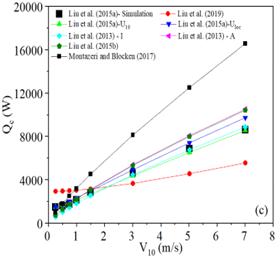
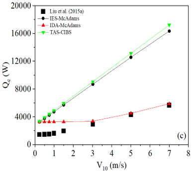
Considering the above fact, the CFD-based results of the heat transfer coefficient (as presented in Figure 1) of Liu et al. [37] are used as a reference as all relevant information is explicitly available and other CHTCs are compared with it. They have used LES with Smagorinsky-Lily subgrid model. Their model is based on the following assumptions; 1) a regular array of the three-story cubical building (10 m 10 m 10 m) comprising of three rows (as shown in Figure 1) immersed in a boundary layer with and without buoyancy effect, 2) the impact of flow regimes on CHTC are accounted by considering four different area plane densities (λp = 0.04, 0.11, 0.25, and 0.44), the effect of sun shading and wind sheltering, 4) the prevailing air is perpendicular to the surface of selected buildings. The temperature difference (ΔT) is considered as 5℃, 10℃ and 15℃ and the velocity at the inlet of computational domain is 5 m/s. They have confirmed results with the wind tunnel experimental data of Meinders et al. [86]) and observed that simulated results show good agreement with experimental data with an average error of less than 10%. In the current CHTC assessment, ΔT = 5℃, and 10℃, and λp = 0.11 and 0.25 are used along with wind velocity obtained from CFD investigation.
To investigate the dynamic performance of correlations collected in Table 1, local weather data (i.e., Qatar) are used. These data are recorded using the solar energy driven HOBO (E-348-RX3000 series) weather station installed at Marina district in Lusail City (25.4254° N, 51.5045° E), Qatar. The Marina district, the targeted area of the current project, is developing part of the Lusail City, and it encompass103 high-rise building stock including commercial, residential, and mix-use buildings with an average height of ~100 m. The weather station provides information on the solar radiation, temperature, and humidity, wind speed, and direction, precipitation, using silicon pyranometer (E-348-S-LIB-M003), temp/RH sensor (E-348-S-THB-M002/M008), wind smart sensor Set (E-348-S-WSET-B), and rain gauge (E-348-S-RGB-M002), respectively. The weather station is confirmed with Fluke 971 multifunction meter and shows the relative average error below 5.5% for dry bulb temperature, relative humidity and dew point temperature.
Figure 1. Heat transfer coefficient variation of Liu et al. [37] used in the current study under different input conditions for the different surfaces (after Liu et al. [37] with permission)
In a dynamic analysis of convective thermal load prediction (the term “dynamic” is referred to the variation during entire day), it is assumed that wind velocity and temperature measured by the weather station are close to the surface of the building, which is certainly not the case in the Marina district. However, this will enable the investigation of the performance of CHTCs and associated convective thermal load under Qatari weather. The temperature difference (ΔT) is 5℃ where the surface temperature is greater than the air temperature. The prevailing wind velocity is assumed to be same for all three surfaces under consideration irrespective of surface orientation and is perpendicular to the surface of the building. The prevailing wind velocity is equal to the wind velocity measured by the weather station. Qatar’s hot weather conditions for 120 h (five days) from August 1 to August 5, 2020, are used. The deviation between simulated results of Liu et al. [37] and calculated cooling loads are expressed in terms of mean absolute percentage error (MAPE) and is calculated using Eq. (2).
MAPE $=\frac{1}{n} \sum_1^n\left|\frac{Q_{c, \text { simulation}} \quad \, -Q_{c, \text { predicted }}}{Q_{\text {c,simulation }}} \quad \right| \times 100 \%$ (2)
where, Qc,predicted is the thermal load calculated using Eq. (1), in which hc is the CHTC listed in the Tables 1 and 2. Qc,simulation is thermal load again using Eq. (1) but based on the CHTC value of Liu et al. [37].
3.1 Assessment of convective heat transfer coefficient correlations developed using urban microclimate
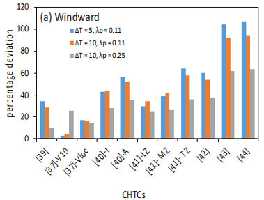
The variation of the associated convective heat energy is presented in Figure 2 for the windward, leeward and roof surface under ΔT = 5℃, λp = 0.11 case, and a detailed error summary for all three cases under consideration (i.e. ΔT = 5℃ and λp = 0.11; ΔT = 5℃, λp = 0.25; ΔT = 10℃, λp = 0.11) with respect to Liu et al’s [37] data are presented in Figure 3. It is observed that,
In the case of windward surface (Figure 2(a) and Figure 3(a)), the correlations of Liu et al. [37] (i.e., V10 and Vloc) shows close predictions with a deviation of 2.5% and 16.9% under ΔT = 5℃, λp = 0.11 and 3.6% and 16.4% under ΔT = 10℃, λp = 0.11. However, the correlation based on V10 shows deviation of 25.5% under ΔT = 10℃, λp = 0.25, while Vloc based correlation meagrely deviates by 14.8%. Correlation of Montazeri and Blocken [44] shows maximum deviation of 107.1% under ΔT = 5℃, λp = 0.11, 57.57% under ΔT = 10℃, λp = 0.11, and 63.3% under ΔT = 10℃, λp = 0.25, as shown in Figure 3(a).
In the case of leeward surface (Figure 2(b)), the correlation of Montazeri and Blocken [44] shows maximum deviation with over-prediction at higher velocity followed by Liu et al. [42] correlation and Liu et al. [40] correlation developed considering the array of the building. However, both correlations of Liu et al. [37] shows close prediction ability with small deviation; 13.2% under ΔT = 5℃, λp = 0.11, 12.2% under ΔT = 10℃, λp = 0.11 and 6.7% under ΔT = 10 ℃, λp = 0.25, as shown in Figure 3(b).
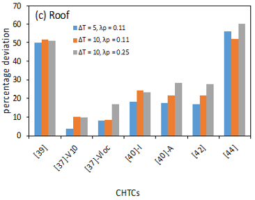
For roof (Figure 2(c)), the deviation of Montazeri and Blocken [44] correlation is maximum with deviation lies between 52.1% to 60.2% under given input conditions as shown in Figure 3(c). The V10 and Vloc based CHTC correlation of Liu et al. [37] shows a closer prediction with simulation results.
Collectively, it is observed that convective energy predictions using each correlation presented in Table 1 deviate under different input conditions and different surface orientations. Among available CHTC correlations, predicted convective load by Liu et al. [37] correlation in terms of Vloc shows the closest prediction (with deviation less than 13% in many cases) to the simulation results, followed by another correlation developed in terms of V10 with deviation less than 16% in many cases. The correlation of Montazeri and Blocken [44] consistently shows a larger deviation (over 48% in all cases) among all correlations for all three surface orientations and input conditions. The closest prediction ability of Liu et al.’s correlation is attributed to the consideration of plane are density (λp) in CHTC development. This accounts for the sun shading and wind sheltering effect experienced due to adjacent buildings.
In urban areas, the presence of neighbouring buildings decreases the heat gain of building surface and surface temperature due to the shading effect [87]. Similarly, sheltering effect triggered from neighbouring buildings reduces local wind speed [40] or the local wind speed increases due to wind channelling resulted from the deepening of a canyon [88, 89]. In Liu et al.’s correlation, these effects of sheltering and sun shading are considered by relating it with plane area density along with local wind velocity and surface temperature. Furthermore, the correlations are sensitive to the velocity (V10 or Vloc), temperature difference (ΔT), and area density ratio (λp), and deviation increases with the increase in the value of these variables. However, it would be inexact to draw this conclusion based on limited set of data.
Figure 2. Variation of convective thermal load for different surface orientations at ΔT = 5, λp = 0.11; a) windward, b) leeward, and c) roof. A = array of buildings, I = isolated building, ML = middle zone, LZ = bottom zone, TZ = top zone
Figure 3. Percentage of deviation of convective thermal load associated with CHTCs from CFD results of Liu et al. [37] under different operating conditions and surface orientations. On X-axis, [39] = Liu et al. [39], [37]- V10 = Liu et al.’s [37] V10 based model, [37]- Vloc = Liu et al’s [37] Vloc based model, [40]-I = Liu et al’s [40] isolated building based model, [40]-A = Liu et al’s [40] array of building based model, [41]-LZ = Kahsay et al’s [41] lower zone model, [41]-MZ = Kahsay et al’s [41] middle zone model, [41]-TZ = Kahsay et al’s [41] top zone model
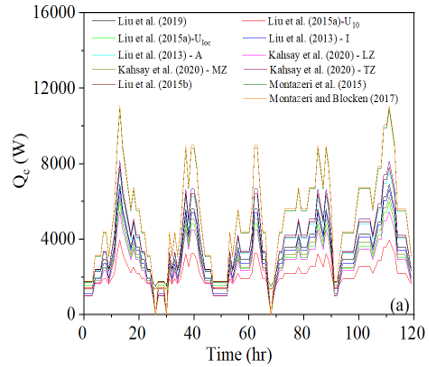
Figure 4. Variation of the CHTCs in Table 1 for Qatar’s weather condition (form August 1 to 5, 2020), (a) windward, (b) leeward, (c) roof. A = array of buildings, I = isolated building, ML = middle zone, LZ = bottom zone, TZ = top zone
3.2 Dynamic variation of convective heat transfer coefficient correlations developed from urban microclimate
Figure 4 shows the variations in the convective thermal load associated with different CHTC correlations (compiled in Table 1) for Qatar’s hot weather conditions for 120 h (five days) from August 1 to August 5, 2020. All correlations show a strong dependency on the wind speed for all surfaces under consideration, namely, windward, leeward, roof. The correlations show significant deviation from each other for the windward surface.
Figure 3 reflects the convective heat transfer rate to the surface and possible impact on corresponding energy consumption estimation associated with convective heat transfer mode concerning time (diurnal and nocturnal) for Qatari weather conditions. It is observed that,
At the peak velocity during the daytime, the correlation of Montazeri and Blocken [44] and Montazeri et al. [43] consistently shows the maximum value of the convective thermal load for the windward, leeward, and roof surface, as shown in Figure 4. Whereas Liu et al.’s [37] correlation developed in terms of V10, Liu et al. [42] and Liu et al. [39] give the lowest value for the windward, leeward and roof surface.
When the wind velocity is very low (the measurement accuracy of the velocity is ±1.1 m/s or 4% of the reading, whichever is greater), the correlations of Liu et al. [39] and Liu et al. [37] show a non-zero thermal load value for the windward, leeward, and roof surface, unlike other correlations. The temperature difference is a crucial factor since there is always an existence of heat transfer due to natural convection, although the wind velocity is close to zero.
The difference between the maximum and minimum thermal load for 24 h is more for Montazeri and Blocken [44]. The lower difference is observed for Liu et al.’s [37] model developed in terms of V10. These correlations' prediction abilities will be different, although the trend still is the same under different input conditions.
The current analysis shows that a proper selection of CHTC in associated thermal load analysis is important. For instance, Montazeri and Blocken [44] and Liu et al. [42] correlations can significantly increase or decrease the predicted daily energy consumption of the corresponding buildings compared to other correlations, respectively. This enforces the engineer to design an oversized or undersized HVAC system depending on the CHTCs. Former adds economic dissatisfaction and later creates discomfort to the end-user. However, actual data of the thermal load and the measured temperature and velocity near the building surface are needed to support the choice of the proper CHTC from Qatar’s context.
3.3 Assessment of convective heat transfer coefficient correlations used in Building Energy Simulation tools
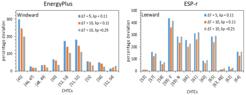
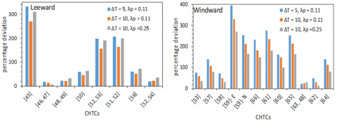
The variation of the different CHTC correlations in Table 2 is studied and compared with the simulation results of Liu et al.’s [37] results for different ΔT and λp. This comparison is made for the windward, leeward, and roof surfaces. Figure 5 presents the variation of the convective thermal load associated with different CHTCs for ΔT = 5℃ and λp = 0.11, for windward surface and detailed error summary under all ΔT and λp cases for all three surfaces is presented in Figure 6 and 7. It is observed that,
In the case of the EnergyPlus, all correlations show over prediction for windward surface, except the prediction TARP model shown in Figure 5(a). The TARP algorithm shows deviation less than 26% for all windward, leeward, and roof surfaces. Also, the Mitchell correlation shows a second better prediction ability for the windward surface with deviation of less than 30.1%. However, the MoWiTT algorithm shows a second good prediction for leeward and roof surfaces deviates by 35.7%, among other correlations. The simpleCombined model consistently shows maximum deviation of over 200% for all cases under consideration and the windward, leeward, and roof surfaces, as presented in Figure 6.
Figure 5. Variation of CHTCs of different BES for windward surface (a) EnergyPlus, (b) ESP-r, (c) IES, TAS, IDA
Figure 6. Percentage of deviation of convective thermal load associated with CHTCs, from CFD results of Liu et al. [37], used in EnergyPlus and Environmental Systems Performance - Research (ESP-r) under different operating conditions and surface orientations
In the case of the ESP-r, all correlations show over prediction for the windward surface, as shown in Figure 5(b). the MoWiTT correlation show close prediction ability with deviation less than 30% for the windward surface. The predicted convective thermal load for leeward surface using McAdam’s correlations is closer to that of Liu et al.’ data compared to MoWiTT correlations. Liu and Harris's correlation shows a closer prediction deviation of less than 23.2% for roof surface, among other correlations. On the contrary, the Sturrock correlation developed for exposed surface consistently shows maximum deviation with deviation of more than 241.1% for all cases, as shown in Figure 6.
In the case of the IES, IDA, and TAS, as presented in Figure 5(c) for windward surface, each one has only one model for each tool, and that shows over prediction with a large deviation compared to that of Liu et al.’s data for windward, leeward and roof surface. The corresponding error for all three differently oriented surfaces and input conditions are presented in Figure 7.
In case of CHTCs in BES tools (CHTCs presented in Table 2), from Figure 6, the TARP shows overall better prediction ability (with deviation less than 26%) for windward, leeward, and roof surface in the case of the EnergyPlus tool. The MoWiTT and Mitchell correlations could be a second choice. The superior prediction capability of TARP can be supported in favour buoyancy effect which is accounted for by surface tilt angle [30] and consideration of wind speed and surface temperature [90]. The SimpleCombined model shows a large deviation for wind, leeward, and roof surfaces, which is in line with earlier studies (cf. [91]). However, in the case of the ESP-r, different correlations show a close prediction ability for different surfaces. For windward surface: MoWiTT; for leeward surface: MoWiTT and McAdams; and for roof surface: Liu and Harris show closer prediction with deviation less than 30% among other correlations as shown Figure 6.
The correlation used in IES, IDA, and TAS show a large deviation for windward, leeward, and roof surfaces under-considered input conditions, as shown in Figure 7. Among all considered BES tools, the TARP algorithm used in the EnergyPlus shows better prediction ability for windward, leeward, and roof surfaces than all other correlations. The superior prediction ability of TARP can be attributed to the consideration of the wind speed and temperature difference between surface temperature and air temperature. Furthermore, few models show a substantial deviation compared to Liu et al.’s data.
Figure 7. Percentage of deviation of convective thermal load associated with CHTCs, from CFD results of Liu et al. [37], used in Integrated Environmental Solutions Ltd (IES), IDA, and TAS under different operating conditions and surface orientations
In summary, few correlations are available to predict the exterior convective heat transfer coefficient considering the microclimate effect, and the convective thermal load predicted using those correlations show significant deviation. The correlation of Liu et al. [37] and Montazeri and Blocken [44] gives the minimum and maximum deviation in windward, leeward and roof surface under given conditions, respectively. These correlations are developed considering a single building or small urban area, following a numerical approach (i.e., CFD) and generally validated at lab-scale experiments [37, 41].
Although CFD allows explicit coupling between different flow fields (velocity, temperature, humidity, and pollution, etc.) at finer scales [92] and enable to exploit different operational scenarios [93, 94], it requires high-resolution urban geometry, specific knowledge of the boundary conditions of governing variables besides adequate computational resources [93, 95, 96]. However, recent advancements in computing resources enable faster modelling of a big urban area for more correct results (for example, Mortezazadeh and Wang [97]). Similarly, convective thermal load prediction using CHTCs available in BES tools, generally validated and trained using weather data collected at the airport, are subject to large deviation under consideration of microclimate, as they need certain amendments in velocity. Among the considered tools, the MoWiTT algorithm show closer prediction ability with deviation of less than 30% for windward, leeward, and roof surface. On the contrary, in the case of the ESP-r, different correlations show a good prediction ability for different surfaces. The IES, IDA, and TAS have few inbuilt correlations (generally one) and show considerable deviation. The literature confirmed that even a slight change in building geometry could affect the CHTC value (Montazeri et al. [43] developed different correlations for different building height and width combinations) and could lead to an imprecise forecast of the real building's energy consumption.
Hence, these correlations may need to validated using real and large-scale measurements (i.e., field measurements), which would perhaps be complicated and costly [42]. Additionally, significantly large size of surfaces and limited access to the building surfaces the CHTC can only be estimated for specific surfaces in the field measurement. However, such measurements are highly recommended in future from perspective of emerging concept of green building. The Gulf Cooperation Council (GCC) countries have many newly constructed and upcoming high-rise buildings together forming a district [98], and their thermal comfort is achieved through centrally located district cooling plants. The inherent hot and arid weather of such countries significantly affects the convective thermal load of high-rise buildings due to elevated temperature over the largest period of a year. These circumstances eventually influence the energy consumption of the district cooling plants since the capacity of the district cooling plant is enormous [38]. Any misjudgement in thermal load predictions of the high-rise buildings in such countries can lead to oversizing of associated district cooling plant that carries substantial capital, maintenance and running cost [99]. The cost associated with the field measurement for development and validation of CHTC to predict convective thermal load more accurately could be significantly lower than that of added capital and operational (running and maintenance) cost due to oversizing of district cooling plant. Moreover, the development of such CHTC could apply to many new developments (i.e., high-rise buildings) in that region, for instance, Qatar, due to uniformity in weather conditions over the region/country. Additionally, a several research program in parallel in different countries can be undertake and their findings can be shared to produce generalized CHTC.
The influence of microclimate is not explicitly considered in the development of CHTC in the past, as they are expressive function either of or combination of wind velocity (V, generally measured at the airport), temperature difference (ΔT), and area plan density (λp) as presented by Eq. (3).
$h_c=f\left(V\right.$ and $/$ or $\lambda_p$ and $/$ or $\left.\Delta T\right)$ (3)
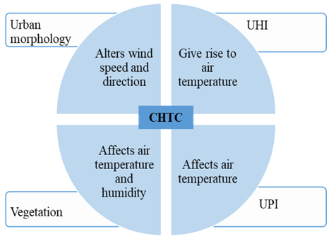
Other effects such are terrain type, roughness index, wind direction, tilt angle, and angle of attack are accounted for by constants. These factors may introduce associated errors in the depiction of convective thermal load, which is always the case, as airflow patterns and their interaction with the building are complicated, varying from region to region. Indeed, the microclimate in the building's vicinity is significantly affected by surrounding complex building morphology, UHI, vegetation, and global warming, as presented in Figure 8.
Figure 8. The intrinsic relationship between influencing factors, microclimate parameter, and CHTC
Generally, building morphology and vegetation hinder the wind flow alters its velocity and direction. On the other hand, air temperature and humidity are directly affected by the UHI and UPI effect, and vegetation. Such a dependency between microclimate and the influencing factors could be accounted for by incorporating representative indicators for each one of these factors. For example, the influence of a UHI effect (UHIindex) can be introduced by the ratio of the air temperature of the urban area (Ta,urban) to the corresponding air temperature of nearby rural development (Ta,rural). This ratio is always greater than zero and is expectedly different from one urban development to another. The effect of vegetation can be introduced through the ratio (Vindex) of the vegetated area to the total area of urban development. Furthermore, the urban air pollution can be accounted for through the urban pollution island index (UPIindex) [100-102], based on the city's overall pollution level where the targeted building is situated or planned to be erect. Such consideration can help the designer to understand the physical interaction of influencing factors to the microclimate and their association with convective heat transfer coefficient.
Few correlations are considered the impact of urban morphology through the area plan density (λp) and the height and width of a particular building. However, this does not stand for the morphology of the complete urban development. The buildings' regional distribution function based on their height and compactness based on street width can be introduced in CHTC correlations. Elnaklah et al. [98] proposed urban morphology (or roughness) parameters that may be useful. In this way, a more generalized and high-quality CHTC can be developed in the form of Eq. (4).
$h_c=f\left(V, \Delta T, U H I_{\text {index }}, M_{\text {index }}, U P I_{\text {index }}, \mathrm{V}_{\text {index }} \right)$ (4)
It is expected that the magnitude of the different indices would be different since the impact of UHI, vegetation, urban morphology, and UPI would be different for different cities and countries. Hence, researchers and scientist from the different countries should work in collaboration to quantify the impact of aforementioned parameters or to identify another parameter if any. Incorporating such indexes is encouraged to help the designer understand the physical interaction of influencing factors to the microclimate and their association with the convective thermal load. Consequently, the building’s energy consumption associated with convective heat transfer at the design stage can be minimized.
Based on the current analysis, the following conclusions are made:
Among available CHTC correlations considering microclimate (generally CFD-based), Liu et al. [37] correlation show the closest predicted convective thermal load to the simulation results with deviation less than 30%, and other correlations consistently show a large deviation such as Montazeri and Blocken [44] exhibits deviation more than 50%. Furthermore, the correlations are sensitive to the velocity, temperature difference (ΔT), area density ratio (λp), and deviation increases with the increase in these variables' value.
Dynamic variation of the CHTCs for Qatar’s weather data is investigated and observed that these correlations show significant variation among each other. These correlations' prediction abilities will be different, although the trend still is the same under different input conditions. However, in the absence of real data, it is difficult to conclude about the superiority of these correlations from Qatar’s context. However, Montazeri and Blocken's [44] correlation can significantly increase the estimated daily energy consumption of the corresponding buildings compared to other correlations.
In the case of the correlations used EnergyPlus, it is observed that the TARP shows overall better prediction ability (with deviation of less than 26%) for windward, leeward, and roof surface. TARP's superior prediction ability can be attributed to considering the wind speed and temperature difference between surface temperature and air temperature. On the other hand, in the case of the ESP-r, different correlations show an excellent prediction ability for different surfaces. For windward surface: MoWiTT; for leeward surface: MoWiTT and McAdams; and for roof surface: Liu and Harris show closer prediction with deviation less than 30% among other correlations. The correlations used in IES, IDA, and TAS show a large deviation for windward, leeward, and roof surfaces among considered inputs.
Improper choice of CHTC in predicting the convective heat transfer rate can lead to a significant over prediction, which would eventually affect the building's energy consumption. Hence, further attention is needed to increase their prediction ability by:
Developing CHTC correlations considering the whole district using modern computing resources i.e., CFD.
Validating and modifying or redefining existing CHTC based on real field measurement data considering flow field around the building.
Incorporation of factors affecting the microclimate such as urban morphology, vegetation, urban heat island, and urban pollution level in CHTC development.
This paper was made possible by an NPRP award [#NPRP11S-1208-170073] from the Qatar National Research Fund (a member of The Qatar Foundation). The statements made herein are solely the responsibility of the authors.
|
δ |
atmospheric boundary layer thickness at a building site (m) |
|
δf |
atmospheric boundary layer thickness at a weather station (m) |
|
η |
weighting factor for natural convection |
|
θ |
angle of incidence between wind and surface, angle of attack (degree) |
|
λp |
area plan density ratio |
|
μ |
dynamic viscosity (N·s/m2) |
|
ρ |
air density (kg/m3) |
|
φ |
surface tilt angle (degree) |
|
Σ |
surface tilt angle (radian) |
|
A |
Area (m2) |
|
BES |
building energy simulation |
|
BLAST |
Building Loads Analysis and System Thermodynamics |
|
C |
wind speed profile exponent at the site |
|
Cf |
wind speed profile exponent at the meteorological station |
|
CIBS |
Chartered Institute of Building Services |
|
D, E, F |
material roughness coefficients |
|
DOE |
Department of energy |
|
GrLn |
Grashof number |
|
H |
building height (m) |
|
hc, CHTC |
convective heat transfer coefficient (W/(m2·K)) |
|
hc,glass |
convective heat transfer coefficient for very smooth surface (W/(m2·K)) |
|
hf |
forced convective heat transfer coefficient (W/(m2·K)) |
|
hn |
natural convective heat transfer coefficient (W/(m2·K)) |
|
HVAC |
heating ventilation and air conditioning |
|
IES |
Integrated Environmental Solutions |
|
MoWiTT |
Mobile Window Thermal Test |
|
k |
thermal conductivity of air (W/(m·K)) |
|
P |
perimeter of surface (m) |
|
Pr |
Prandtl number |
|
RaLn |
Rayleigh number |
|
Re |
Reynolds number |
|
Rf |
surface roughness multiplier |
|
ΔT |
temperature difference between surface and air (℃) |
|
TARP |
Thermal Analysis Research Program |
|
TAS |
Thermal Analysis Software |
|
To |
exterior surface temperature (℃) |
|
Ta |
ambient air temperature (℃) |
|
V10 |
wind velocity at 10 m height (m/s) |
|
Vloc |
local wind velocity (m/s) |
|
Vmet |
velocity at meteorological station (m/s) |
|
Vr |
roof wind speed (m/s) |
|
Vz |
local wind speed calculated at the height above ground of the surface centroid (m/s) |
|
W |
building width (m) |
|
x |
distance to the surface centroid from where the wind begins to intersect the roof (m) |
|
Z |
height above ground level (m) |
[1] UNDESA, 2014, UNDESA, https://www.un.org/en/development/desa/news/population/world-urbanization-prospects.html, accessed on 26/02/2022.
[2] Lin, L., Luo, M., Chan, T. O., Ge, E., Liu, X., Zhao, Y., Liao, W. (2019). Effects of urbanization on winter wind chill conditions over China. Science of the Total Environment, 688: 389-397. https://doi.org/10.1016/j.scitotenv.2019.06.145
[3] Mariano-Hernández, D., Hernández-Callejo, L., Zorita-Lamadrid, A., Duque-Pérez, O., García, F.S. (2021). A review of strategies for building energy management system: Model predictive control, demand side management, optimization, and fault detect & diagnosis. Journal of Building Engineering, 33: 101692. https://doi.org/10.1016/j.jobe.2020.101692
[4] Yu, J., Tian, L., Xu, X., Wang, J. (2015). Evaluation on energy and thermal performance for office building envelope in different climate zones of China. Energy and Buildings, 86: 626-639. https://doi.org/10.1016/j.enbuild.2014.10.057
[5] Isaac, M., Van Vuuren, D.P. (2009). Modeling global residential sector energy demand for heating and air conditioning in the context of climate change. Energy Policy, 37(2): 507-521. https://doi.org/10.1016/j.enpol.2008.09.051
[6] Shibuya, T., Croxford, B. (2016). The effect of climate change on office building energy consumption in Japan. Energy and Buildings, 117: 149-159. https://doi.org/10.1016/j.enbuild.2016.02.023
[7] Yang, X.S., Zhao, L.H., Bruse, M., Meng, Q.L. (2012). Assessing the effect of microclimate on building energy performance by co-simulation. In Applied Mechanics and Materials, 121: 2860-2867. https://doi.org/10.4028/www.scientific.net/AMM.121-126.2860
[8] Yang, X., Zhao, L., Bruse, M., Meng, Q. (2012). An integrated simulation method for building energy performance assessment in urban environments. Energy and Buildings, 54: 243-251. https://doi.org/10.1016/j.enbuild.2012.07.042
[9] Merlier, L., Frayssinet, L., Johannes, K., Kuznik, F. (2019). On the impact of local microclimate on building performance simulation. Part II: Effect of external conditions on the dynamic thermal behavior of buildings. Building Simulation, 12: 747-757. https://doi.org/10.1007/s12273-019-0508-6
[10] Hamdan, D.M.A., De Oliveira, F.L. (2019). The impact of urban design elements on microclimate in hot arid climatic conditions: Al Ain City, UAE. Energy and Buildings, 200: 86-103. https://doi.org/10.1016/j.enbuild.2019.07.028
[11] Toparlar, Y., Blocken, B., Maiheu, B., Van Heijst, G.J.F. (2018). Impact of urban microclimate on summertime building cooling demand: A parametric analysis for Antwerp, Belgium. Applied Energy, 228: 852-872. https://doi.org/10.1016/j.apenergy.2018.06.110
[12] Howard, L. (1833). The climate of London: deduced from meteorological observations made in the metropolis and at various places around it (Vol. 3). Harvey and Darton, J. and A. Arch, Longman, Hatchard, S. Highley [and] R. Hunter.
[13] Oke, T.R. (1973). City size and the urban heat island. Atmospheric Environment (1967), 7(8): 769-779. https://doi.org/10.1016/0004-6981(73)90140-6
[14] Carpio, M., González, Á., González, M., Verichev, K. (2020). Influence of pavements on the urban heat island phenomenon: A scientific evolution analysis. Energy and Buildings, 226: 110379. https://doi.org/10.1016/j.enbuild.2020.110379
[15] Allegrini, J., Carmeliet, J. (2017). Coupled CFD and building energy simulations for studying the impacts of building height topology and buoyancy on local urban microclimates. Urban Climate, 21: 278-305. https://doi.org/10.1016/j.uclim.2017.07.005
[16] Allegrini, J., Dorer, V., Carmeliet, J. (2015). Coupled CFD, radiation and building energy model for studying heat fluxes in an urban environment with generic building configurations. Sustainable Cities and Society, 19: 385-394. https://doi.org/10.1016/j.scs.2015.07.009
[17] Bowen, A., Kasathko, V. (1981). 13 - Heating and Cooling of Buildings Through Landscape Design. In Solar Energy Conversion II (pp. 159-203). Pergamon. https://doi.org/10.1016/B978-0-08-025388-6.50030-1
[18] Wong, N.H., Peck, T.T. (2005). The impact of vegetation on the environmental conditions of housing estates in Singapore. International Journal on Architectural Science, 6(1): 31-37.
[19] Hoelscher, M.T., Nehls, T., Jänicke, B., Wessolek, G. (2016). Quantifying cooling effects of facade greening: Shading, transpiration and insulation. Energy and Buildings, 114: 283-290. https://doi.org/10.1016/j.enbuild.2015.06.047
[20] Susorova, I., Azimi, P., Stephens, B. (2014). The effects of climbing vegetation on the local microclimate, thermal performance, and air infiltration of four building facade orientations. Building and Environment, 76: 113-124. https://doi.org/10.1016/j.buildenv.2014.03.011
[21] Sternberg, T., Viles, H., Cathersides, A. (2011). Evaluating the role of ivy (Hedera helix) in moderating wall surface microclimates and contributing to the bioprotection of historic buildings. Building and Environment, 46(2): 293-297. https://doi.org/10.1016/j.buildenv.2010.07.017
[22] Gunawardena, K., Steemers, K. (2021). Living wall influence on the microclimates of sheltered urban conditions: results from monitoring studies. Architectural Science Review, 64(3): 235-246. https://doi.org/10.1080/00038628.2020.1812501
[23] Ulpiani, G. (2021). On the linkage between urban heat island and urban pollution island: Three-decade literature review towards a conceptual framework. Science of the Total Environment, 751: 141727. https://doi.org/10.1016/j.scitotenv.2020.141727
[24] Allen-Dumas, M.R., Rose, A.N., New, J.R., Omitaomu, O.A., Yuan, J., Branstetter, M.L., Sylvester, L.M., Seals, M.B., Carvalhaes, T.M., Adams, M.B., Bhandari, M.S., Shrestha, S.S., Sanyal, J., Berres, A.S., Kolosna, C.P., Fu, K.S., Kahl, A.C. (2020). Impacts of the morphology of new neighborhoods on microclimate and building energy. Renewable and Sustainable Energy Reviews, 133: 110030. https://doi.org/10.1016/j.rser.2020.110030
[25] Salata, F., Golasi, I., de Lieto Vollaro, A., de Lieto Vollaro, R. (2015). How high albedo and traditional buildings’ materials and vegetation affect the quality of urban microclimate. A case study. Energy and Buildings, 99: 32-49. https://doi.org/10.1016/j.enbuild.2015.04.010
[26] Xiao, Z., Gang, W., Yuan, J., Zhang, Y., Fan, C. (2021). Cooling load disaggregation using a NILM method based on random forest for smart buildings. Sustainable Cities and Society, 74: 103202. https://doi.org/10.1016/j.scs.2021.103202
[27] Chua, K.J., Chou, S.K. (2010). Energy performance of residential buildings in Singapore. Energy, 35(2): 667-678. https://doi.org/10.1016/j.energy.2009.10.039
[28] Kwan, Y., Guan, L. (2015). Design a zero energy house in Brisbane, Australia. Procedia Engineering, 121: 604-611. https://doi.org/10.1016/j.proeng.2015.08.1046
[29] Chen, Z., Qu, M. (2016). Model-based Building Performance Evaluation and Analysis for a New Athletic Training Facility. Procedia Engineering, 145: 884-891. https://doi.org/10.1016/j.proeng.2016.04.115
[30] EnergyPlus v9.1.0, 2019. https://bigladdersoftware.com/projects/energyplus/, accessed on December 1, 2022.
[31] Beausoleil-Morrison, I. (2001). An algorithm for calculating convection coefficients for internal building surfaces for the case of mixed flow in rooms. Energy and Buildings, 33(4): 351-361. https://doi.org/10.1016/S0378-7788(00)00117-1
[32] Beausoleil-Morrison, I. (1999). Modelling mixed convection heat transfer at internal building surfaces. In Building Simulation (Vol. 99).
[33] Mirsadeghi, M., Costola, D., Blocken, B., Hensen, J.L. (2013). Review of external convective heat transfer coefficient models in building energy simulation programs: Implementation and uncertainty. Applied Thermal Engineering, 56(1-2): 134-151. https://doi.org/10.1016/j.applthermaleng.2013.03.003
[34] Liu, J., Heidarinejad, M., Gracik, S., Jareemit, D., Srebric, J. (2014). The impact of surface convective heat transfer coefficients on the simulated building energy consumption and surface temperatures. Hong Kong.
[35] Ciancio, V., Falasca, S., Golasi, I., Curci, G., Coppi, M., Salata, F. (2018). Influence of input climatic data on simulations of annual energy needs of a building: EnergyPlus and WRF modeling for a case study in Rome (Italy). Energies, 11(10): 2835. https://doi.org/10.3390/en11102835
[36] Ramponi, R., Blocken, B., de Coo, L.B., Janssen, W.D. (2015). CFD simulation of outdoor ventilation of generic urban configurations with different urban densities and equal and unequal street widths. Building and Environment, 92: 152-166. https://doi.org/10.1016/j.buildenv.2015.04.018
[37] Liu, J., Heidarinejad, M., Gracik, S., Srebric, J. (2015). The impact of exterior surface convective heat transfer coefficients on the building energy consumption in urban neighborhoods with different plan area densities. Energy and Buildings, 86: 449-463. https://doi.org/10.1016/j.enbuild.2014.10.062
[38] Kadam, S.T., Hassan, I., Rahman, M.A., Papadopoulos, A.I., Seferlis, P. (2020). Review on modeling of vapor compression chillers: District cooling perspective. International Journal of Air-Conditioning and Refrigeration, 28(2): 2030003. https://doi.org/10.1142/S2010132520300037
[39] Liu, J., Heidarinejad, M., Nikkho, S.K., Mattise, N.W., Srebric, J. (2019). Quantifying impacts of urban microclimate on a building energy consumption—a case study. Sustainability, 11(18): 4921. https://doi.org/10.3390/su11184921
[40] Liu, J., Srebric, J., Yu, N. (2013). Numerical simulation of convective heat transfer coefficients at the external surfaces of building arrays immersed in a turbulent boundary layer. International Journal of Heat and Mass Transfer, 61: 209-225. https://doi.org/10.1016/j.ijheatmasstransfer.2013.02.005
[41] Kahsay, M. T., Bitsuamlak, G., Tariku, F. (2020). Effect of localized exterior convective heat transfer on high-rise building energy consumption. In Building Simulation, 13: 127-139. https://doi.org/10.1007/s12273-019-0568-7
[42] Liu, J., Heidarinejad, M., Gracik, S., Srebric, J., Yu, N. (2015). An indirect validation of convective heat transfer coefficients (CHTCs) for external building surfaces in an actual urban environment. In building Simulation, 8: 337-352. https://doi.org/10.1007/s12273-015-0212-0
[43] Montazeri, H., Blocken, B., Derome, D., Carmeliet, J., Hensen, J.L. (2015). CFD analysis of forced convective heat transfer coefficients at windward building facades: Influence of building geometry. Journal of Wind Engineering and Industrial Aerodynamics, 146: 102-116. https://doi.org/10.1016/j.jweia.2015.07.007
[44] Montazeri, H., Blocken, B. (2017). New generalized expressions for forced convective heat transfer coefficients at building facades and roofs. Building and Environment, 119: 153-168. https://doi.org/10.1016/j.buildenv.2017.04.012
[45] Kusuda, T. (1976). Computer program for heating and cooling loads in buildings. Building Science Series, pp. 76-6000. https://nvlpubs.nist.gov/nistpubs/Legacy/IR/nbsir74-574.pdf.
[46] Walton, G.N. (1983). Thermal analysis research program reference manual. National Bureau of Standards, March.
[47] Walton, G.N. (1981). Passive solar extension of the building loads analysis and system thermodynamics (BLAST) program. United States Army Construction Engineering Research Laboratory, Champaign, IL, 40: 41.
[48] Yazdanian, M., Klems, J.H. (1993). Measurement of the exterior convective film coefficient for windows in low-rise buildings. ASHRAE Trans., 100(1): 1-15.
[49] Booten, C., Kruis, N., Christensen, C. (2012). Identifying and resolving issues in energyplus and DOE-2 window heat transfer calculations (No. NREL/TP-5500-55787). National Renewable Energy Lab.(NREL), Golden, CO (United States). https://doi.org/10.2172/1051164
[50] LBL. DOE2.1E-053 Source Code, 1994. https://doe2.com/Download/DOE-21E/DOE-2EngineersManualVersion2.1A.pdf, accessed on December 1, 2022.
[51] Nusselt, W., Jürges, W. (1922). Die Kühlung einer ebenen Wand durch einen Luftstrom (The cooling of a plane wall by an air flow). Gesundheits Ingenieur, 52(45): 641-642.
[52] Palyvos, J.A. (2008). A survey of wind convection coefficient correlations for building envelope energy systems’ modeling. Applied Thermal Engineering, 28(8-9): 801-808. https://doi.org/10.1016/j.applthermaleng.2007.12.005
[53] McAdams, W.H. (1954). Heat Transmission. McGraw-hill.
[54] Mitchell, J.W. (1976). Heat transfer from spheres and other animal forms. Biophysical Journal, 16(6): 561-569. https://doi.org/10.1016/S0006-3495(76)85711-6
[55] Blocken, B., Defraeye, T., Derome, D., Carmeliet, J. (2009). High-resolution CFD simulations for forced convective heat transfer coefficients at the facade of a low-rise building. Building and Environment, 44(12): 2396-2412. https://doi.org/10.1016/j.buildenv.2009.04.004
[56] Emmel, M.G., Abadie, M.O., Mendes, N. (2007). New external convective heat transfer coefficient correlations for isolated low-rise buildings. Energy and Buildings, 39(3): 335-342. https://doi.org/10.1016/j.enbuild.2006.08.001
[57] Chartered Institute of Building Services (CIBS). (1979). A guide book, Section A3.
[58] Jayamaha, S.E.G., Wijeysundera, N.E., Chou, S.K. (1996). Measurement of the heat transfer coefficient for walls. Building and Environment, 31(5): 399-407. https://doi.org/10.1016/0360-1323(96)00014-5
[59] Sturrock, N.S. (1971). Localized boundary-layer heat transfer from external building surfaces. Doctoral dissertation, University of Liverpool.
[60] Loveday, D.L., Taki, A.H. (1996). Convective heat transfer coefficients at a plane surface on a full-scale building facade. International Journal of Heat and Mass Transfer, 39(8): 1729-1742. https://doi.org/10.1016/0017-9310(95)00268-5
[61] Nicol, K. (1977). The energy balance of an exterior window surface, Inuvik, NWT, Canada. Building and Environment, 12(4): 215-219. https://doi.org/10.1016/0360-1323(77)90022-1
[62] Liu, Y., Harris, D.J. (2007). Full-scale measurements of convective coefficient on external surface of a low-rise building in sheltered conditions. Building and Environment, 42(7): 2718-2736. https://doi.org/10.1016/j.buildenv.2006.07.013
[63] Klems, J.H., Selkowitz, S., Horowitz, S. (1981). Mobile facility for measuring net-energy performance of windows and skylights (No. LBL-12765; CONF-820309-3). Lawrence Berkeley Lab., CA (USA).
[64] BS EN ISO 6946:2017 Building components and building elements - thermal resistance and thermal transmittance - calculation method. 1997. British Standards Institution, UK.
[65] Hagishima, A., Tanimoto, J. (2003). Field measurements for estimating the convective heat transfer coefficient at building surfaces. Building and Environment, 38(7): 873-881. https://doi.org/10.1016/S0360-1323(03)00033-7
[66] American society of heating refrigerating and air conditioning engineers. (1976). Procedures for Determining Heating and Cooling Loads for Computering Energy Calculations: Algorithms for Building Heat Transfer Subroutines/Compil Ed by Subcommittee for Heating and Cooling Loads ASHRAE Task Group on Energy Requirements. ASHRAE.
[67] ASHRAE Handbook Fundamentals. 1989. The American Society of Heating, Refrigerating, and Air Conditioning Engineers, Inc, USA.
[68] ASHRAE Handbook: 1981 Fundamentals. 1989. Atlanta: American Society of Heating, Refrigerating, and Air-Conditioning Engineers, Inc, USA.
[69] Clear, R. D., Gartland, L., Winkelmann, F. C. (2003). An empirical correlation for the outside convective air-film coefficient for horizontal roofs. Energy and Buildings, 35(8): 797-811. https://doi.org/10.1016/S0378-7788(02)00240-2
[70] Sharples, S. (1984). Full-scale measurements of convective energy losses from exterior building surfaces. Building and Environment, 19(1): 31-39. https://doi.org/10.1016/0360-1323(84)90011-8
[71] Ito, N. (1972). Field experiment study on the convective heat transfer coefficient on exterior surface of a building. ASHRAE Trans.;(United States), 78: 184-191.
[72] Clarke, J. (2007). Energy Simulation in Building Design. Routledge.
[73] Cai, R., Zhang, N. (2003). Explicit analytical solutions of 2-D laminar natural convection. International Journal of Heat and Mass Transfer, 46(5): 931-934. https://doi.org/10.1016/S0017-9310(02)00359-9
[74] Massabó, M., Cianci, R., Paladino, O. (2006). Some analytical solutions for two-dimensional convection–dispersion equation in cylindrical geometry. Environmental Modelling & Software, 21(5): 681-688. https://doi.org/10.1016/j.envsoft.2004.12.003
[75] Toja-Silva, F., Kono, T., Peralta, C., Lopez-Garcia, O., Chen, J. (2018). A review of computational fluid dynamics (CFD) simulations of the wind flow around buildings for urban wind energy exploitation. Journal of Wind Engineering and Industrial Aerodynamics, 180: 66-87. https://doi.org/10.1016/j.jweia.2018.07.010
[76] Du, Y., Mak, C.M., Liu, J., Xia, Q., Niu, J., Kwok, K.C. (2017). Effects of lift-up design on pedestrian level wind comfort in different building configurations under three wind directions. Building and Environment, 117: 84-99. https://doi.org/10.1016/j.buildenv.2017.03.001
[77] Tabrizi, A.B., Whale, J., Lyons, T., Urmee, T. (2014). Performance and safety of rooftop wind turbines: Use of CFD to gain insight into inflow conditions. Renewable Energy, 67: 242-251. https://doi.org/10.1016/j.renene.2013.11.033
[78] Simões, T., Estanqueiro, A. (2016). A new methodology for urban wind resource assessment. Renewable Energy, 89: 598-605. https://doi.org/10.1016/j.renene.2015.12.008
[79] Yang, A.S., Su, Y.M., Wen, C.Y., Juan, Y.H., Wang, W.S., Cheng, C.H. (2016). Estimation of wind power generation in dense urban area. Applied Energy, 171: 213-230. https://doi.org/10.1016/j.apenergy.2016.03.007
[80] Liu, S., Pan, W., Zhang, H., Cheng, X., Long, Z., Chen, Q. (2017). CFD simulations of wind distribution in an urban community with a full-scale geometrical model. Building and Environment, 117: 11-23. https://doi.org/10.1016/j.buildenv.2017.02.021
[81] Tamura, T., Towards practical use of IES in wind engineering. Journal of Wind Engineering and Industrial Aerodynamics, 96(10–11): 1451–1471, 2008. https://doi.org/10.1016/j.jweia.2008.02.034
[82] Sun, S., Wang, H., Zhang, W.W. (2023). Analysis of numerical factors affecting large eddy simulation of pollutant diffusion around buildings. Journal of Wind Engineering and Industrial Aerodynamics, 232: 105244. https://doi.org/10.1016/j.jweia.2022.105244
[83] Xie, Z.T., Castro, I.P. (2009). Large-eddy simulation for flow and dispersion in urban streets. Atmospheric Environment, 43(13): 2174-2185. https://doi.org/10.1016/j.atmosenv.2009.01.016
[84] Chen, J., Elshaer, A., Aboshosha, H., Pedro, G. (2022). Calibrated consistent flow generator for tall building aerodynamics using large eddy simulation. Results in Engineering, 16: 100634. https://doi.org/10.1016/j.rineng.2022.100634
[85] Smolarkiewicz, P.K., Sharman, R., Weil, J., Perry, S.G., Heist, D., Bowker, G. (2007). Building resolving large-eddy simulations and comparison with wind tunnel experiments. Journal of Computational Physics, 227(1): 633-653. https://doi.org/10.1016/j.jcp.2007.08.005
[86] Meinders, E.R., Van der Meer, T.H., Hanjalić, K., Lasance, C.J.M. (1997). Application of infrared thermography to the evaluation of local convective heat transfer on arrays of cubical protrusions. International Journal of Heat and Fluid Flow, 18(1): 152-159. https://doi.org/10.1016/S0142-727X(96)00139-7
[87] Wong, N.H., Jusuf, S.K., Syafii, N.I., Chen, Y., Hajadi, N., Sathyanarayanan, H., Manickavasagam, Y.V. (2011). Evaluation of the impact of the surrounding urban morphology on building energy consumption. Solar Energy, 85(1): 57-71. https://doi.org/10.1016/j.solener.2010.11.002
[88] Battista, G., Evangelisti, L., Guattari, C., Vollaro, R.D. L. (2015). On the influence of geometrical features and wind direction over an urban canyon applying a FEM analysis. Energy Procedia, 81: 11-21. https://doi.org/10.1016/j.egypro.2015.12.054
[89] Pearlmutter, D., Bitan, A., Berliner, P. (1999). Microclimatic analysis of “compact” urban canyons in an arid zone. Atmospheric Environment, 33(24-25): 4143-4150. https://doi.org/10.1016/S1352-2310(99)00156-9
[90] Allegrini, J., Dorer, V., Carmeliet, J. (2012). Analysis of convective heat transfer at building façades in street canyons and its influence on the predictions of space cooling demand in buildings. Journal of Wind Engineering and Industrial Aerodynamics, 104-106: 464-473. https://doi.org/10.1016/j.jweia.2012.02.003
[91] Shen, P., Dai, M., Xu, P., Dong, W. (2019). Building heating and cooling load under different neighbourhood forms: Assessing the effect of external convective heat transfer. Energy, 173: 75-91. https://doi.org/10.1016/j.energy.2019.02.062
[92] Toparlar, Y., Blocken, B., Maiheu, B., Van Heijst, G.J.F. (2017). A review on the CFD analysis of urban microclimate. Renewable and Sustainable Energy Reviews, 80: 1613-1640. https://doi.org/10.1016/j.rser.2017.05.248
[93] Blocken, B. (2015). Computational Fluid Dynamics for urban physics: Importance, scales, possibilities, limitations and ten tips and tricks towards accurate and reliable simulations. Building and Environment, 91: 219-245. https://doi.org/10.1016/j.buildenv.2015.02.015
[94] Kanda, M. (2007). Progress in urban meteorology: A review. Journal of the Meteorological Society of Japan. Ser. II, 85: 363-383. https://doi.org/10.2151/jmsj.85B.363
[95] Mirzaei, P.A., Haghighat, F. (2010). Approaches to study urban heat island–abilities and limitations. Building and Environment, 45(10): 2192-2201. https://doi.org/10.1016/j.buildenv.2010.04.001
[96] Moonen, P., Defraeye, T., Dorer, V., Blocken, B., Carmeliet, J. (2012). Urban Physics: Effect of the micro-climate on comfort, health and energy demand. Frontiers of Architectural Research, 1(3): 197-228. https://doi.org/10.1016/j.foar.2012.05.002
[97] Mortezazadeh, M., Wang, L.L. (2020). Solving city and building microclimates by fast fluid dynamics with large timesteps and coarse meshes. Building and Environment, 179: 106955. https://doi.org/10.1016/j.buildenv.2020.106955
[98] Elnaklah, R., Alnuaimi, A., Alotaibi, B.S., Topriska, E., Walker, I., Natarajan, S. (2021). Thermal comfort standards in the Middle East: Current and future challenges. Building and Environment, 200: 107899. https://doi.org/10.1016/j.buildenv.2021.107899
[99] Khir, R., Haouari, M. (2015). Optimization models for a single-plant District Cooling System. European Journal of Operational Research, 247(2): 648-658. https://doi.org/10.1016/j.ejor.2015.05.083
[100] Li, H., Meier, F., Lee, X., Chakraborty, T., Liu, J., Schaap, M., Sodoudi, S. (2018). Interaction between urban heat island and urban pollution island during summer in Berlin. Science of the Total Environment, 636: 818-828. https://doi.org/10.1016/j.scitotenv.2018.04.254
[101] Crutzen, P.J. (2004). New directions: the growing urban heat and pollution "island" effect-impact on chemistry and climate. Atmospheric Environment, 38(21): 3539-3540.
[102] Darmanto, N.S., Varquez, A.C., Kanda, M. (2017). Urban roughness parameters estimation from globally available datasets for mesoscale modeling in megacities. Urban Climate, 21: 243-261. https://doi.org/10.1016/j.uclim.2017.07.001