Rahmat Safe’i*![]() | Rico Andrian
| Rico Andrian![]() | Diah Adi Sriatna
| Diah Adi Sriatna![]() | Flaurensia Riahta Tarigan
| Flaurensia Riahta Tarigan![]()
© 2024 The authors. This article is published by IIETA and is licensed under the CC BY 4.0 license (http://creativecommons.org/licenses/by/4.0/).
OPEN ACCESS
This article discusses the application of digital image technology and deep learning using Convolutional Neural Network (CNN) in Forest Health Monitoring (FHM). Forest health monitoring is a method for measuring forest health, one of the parameters used is crown density and transparency. Measurement of these parameters is still done manually using magic cards so it is less effective and efficient, so it is necessary to apply digital images, one of which is the CNN algorithm to help measure the density scale and crown transparency. CNN architectures namely AlexNet and VGG16 are used to train the tree image recognition model. This research uses a tree image dataset with four types of needles grouped into classes based on crown density and transparency. The results showed that both CNN architectures achieved a good level of accuracy in classifying coniferous tree species based on crown density and transparency. VGG16 notably achieves higher accuracy than AlexNet. The results of model evaluation via the confusion matrix also provide insight into the model's performance in recognizing crown density and transparency classes.
AlexNet, CNN, deep learning, needle leaves, forest, VGG16
A forest area is a place that consists of various types of trees and is managed by one agency or organization with objectives that are in line with the land owner. In Indonesia, forests produce various forest products, and some of them are the responsibility of the Ministry of Forestry [1]. In Indonesia, forests can be divided into two categories, namely forests that are in good condition and forests that are not in good condition. The health condition of a forest can be seen from the ability of the forest ecosystem to meet the needs of the living creatures in it. Forests are considered to be in good condition when their ecosystem functions are maintained and operating well [2]. Forest health conditions can be observed and monitored using the Forest Health Monitoring (FHM) method [3]. Forest Health Monitoring (FHM) is a systematic process for continuously monitoring and evaluating forest health conditions. This involves collecting data on various parameters that influence forest health, such as live crown ratio, crown density, foliage transparency, crown diameter, and dieback. The main goal is to detect changes in forest conditions early, understand their causes, and plan appropriate management actions to maintain or restore the balance of the forest ecosystem. FHM is carried out using various methods and technologies, including field surveys, remote monitoring with satellites, spatial data analysis, and collaboration with experts and other stakeholders. Thus, FHM becomes an important instrument in sustainable forest management and environmental conservation [4].
The crown density and transparency scale card is used to measure the extent to which sunlight can enter and be filtered by the tree crown. Crown density and transparency are key parameters in assessing forest health. A forest is considered to be in good condition if its crown density reaches or exceeds 55% and its transparency level is in the range between 0 and 45% [5]. Usually, this parameter is assessed manually by an observer who is under the tree being surveyed. The assessment carried out by observers to measure the percentage of crown density and transparency is uniform for all tree types, including coniferous trees. Coniferous trees have a growth pattern that tends to cone upwards, so they tend to block more sunlight from entering the tree's crown area [6]. Currently, implementation using scale cards still tends to be less efficient because it involves visual observation and manual comparison with scale cards. This obstacle can be overcome by involving computing technology, one of which is digital image technology.
Digital image technology can be applied using various methods, including deep learning. Deep learning is a component of machine learning that has the ability to learn its own methods in computing [7]. Deep learning, in particular, presents a very innovative approach to image classification as it expands traditional machine learning concepts by integrating a higher level of ‘depth’ into the model structure [8]. The deep learning method currently used for image recognition is the convolutional neural network (CNN). CNN attempts to mimic the image recognition system of the human visual cortex, which gives it the ability to process image information effectively [9]. CNN has several architectures. The architecture used in this research is AlexNet and VGG16. AlexNet is one of the CNN architectures that won the ImageNet Large Scale Visual Recognition Challenge (ILSVRC) competition, a large-scale image classification competition, in 2012. AlexNet introduces new innovations in the field of deep learning by combining CNN with dropout regularization techniques, using ReLu as an activation function, and utilizing data augmentation [10]. VGG16 is a CNN architecture consisting of 13 convolution layers and 3 fully connected layers with weights, and is capable of processing images with three RGB color channels (Red, Green, and Blue) [11].
This research was conducted in the Tahura WAR Conservation Forest in the Kemiling area of Bandar Lampung. The focus of this research is the use of four types of trees with needle leaves, namely pine merkusii, araucaria heterophylla, cupressus retusa, and shorea javanica. The results of this research can be applied to identify the density and transparency scales of the four types of trees with needle leaves. The information obtained from this research can also be useful for detecting the density and transparency of the canopy of tropical pine and araucaria trees, which are commonly found in tropical rainforests. Thus, the results of this research contribute to the understanding and management of forest ecosystems, especially in the Tahura WAR conservation forest area and similar types of tropical rainforest.
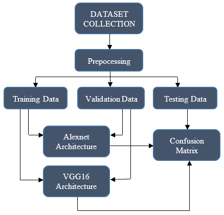
This research uses a data set containing images of trees with needles. This dataset includes four different tree types, with each tree type consisting of 1000 images. Within each tree type, there are ten different density and transparency classes, and each class has 100 relevant images. In total, this dataset consists of 4000 images, which have been grouped into appropriate classes. The steps of this research are explained in Figure 1 [12].
Figure 1. Research flow
2.1 Image collection
The initial stage in the research was taking pictures of coniferous trees as the main data. These images were obtained from the Tahura WAR Kemiling traditional area and the area around the University of Lampung (around the rectorate, the second route area around the UPT ICT, mechanical engineering department, banyan, and physics department). There were four types of needle leaves collected, namely araucaria heterophylla, pine merkusii, cupressus retusa, and shorea javanica. The images were taken using a Canon Eos 250D camera with ISO 200 because the images were taken in an open room so the sensitivity was not too low and not too high by using a ratio of 1 to 1. Only a few images were collected due to the poor growth of the needles and the position of the needles. The terrain is high and uneven, so augmentation is needed to meet the needs for the number of datasets.
2.2 Preprocessing
The next step is to separate the images of coniferous trees into appropriate classes based on their density and transparency. After that, this tree dataset is labeled according to its category and resized to 224x224 pixels [13]. To expand the dataset of coniferous tree images, an augmentation technique was carried out so that each class would have 100 images [14]. Data augmentation is a technique used to create additional variations in the training data by modifying the images. Data augmentation can include rotation, shift, horizontal or vertical flip, zoom, or color change. The augmentation techniques used in this research are flip vertical, flip horizontal, and zoom of 0.1 on each needle leaf crown image. Ultimately, the tree dataset will consist of 4000 images of trees with four different types of needles, where each type has 100 images in each of the 10 categories of crown density and transparency. This needle leaf-type dataset is stored in Google Drive to facilitate data processing with models programmed in Google Collab. The dataset is also stored on a Tesla K80 computer. Each tree-type image is stored in four different folders based on its density and transparency category labels. The machine will read this dataset at the initial stage of the process and then process it according to the categories listed in each folder [15].
2.3 Split data
Each image of data that has been separated based on class is then divided into three main components: training data, validation data, and testing data.
2.3.1 Training data
Training data is used as the main material for carrying out the dataset training process [16]. The training data used was 70% of each dataset per type of coniferous tree.
2.3.2 Validation data
Data validation is used to assist the process of training the dataset using training data. The training process using training data also requires data validation to prove the similarity of the data read by the model [17]. The validation data used in this research was 10% of each dataset per type of coniferous tree.
2.3.3 Testing data
Data testing is used to test datasets on an existing architecture [18]. The testing data used in this research was 20% of each dataset per type of coniferous tree.
2.4 AlexNet and VGG16 architecture training
Training the model involved the use of two architectures, namely AlexNet and VGG16, with a dataset containing 700 images for each needle type. Training of this model was carried out using Google Collab and Jupyter Notebook and involved adjusting hyperparameters such as epoch, batch size, optimizer, and learning rate [19]. These hyperparameter settings have an important role in influencing the success of model training and testing. The hyperparameter values used are in Table 1.
Table 1. Hyperparameter Values
|
Hyperparameter |
AlexNet |
VGG16 |
|
Epoch |
20 |
10 |
|
Batch-size |
8 |
32 |
|
Optimizer |
Adam |
Adam |
|
Learning-rate |
0.0001 |
0.001 |
Model training requires several hyperparameters such as the number of training times (epoch), the amount of data processed at once (batch-size), how large the learning steps are (learning-rate), and the optimization algorithm used (optimizer). Various combinations of these settings are required to achieve the desired results. Training the VGG16 model for the needle leaf dataset, the hyperparameters used are: training is carried out 10 times (epochs), 32 data samples are processed at one time (batch-size 32), the learning rate is very small, namely 0.001, and uses the Adam optimization algorithm. Likewise, when training the AlexNet model, it requires 20 training times (epochs), 8 data samples are processed at one time (batch-size 8), the learning rate is very small, namely 0.0001, and uses the Adam optimization algorithm. With this setup, the model will learn to recognize the dataset when tested. However, sometimes further experimentation is needed to find the most optimal settings for that specific dataset.
2.5 Confusion Matrix
The confusion matrix is obtained after going through the model training stage on training and validation data. When testing a model, test data is used to evaluate the performance of a model that has undergone previous training. Performance assessment of these two models can be done using a confusion matrix to calculate various metrics such as accuracy, F1-score, recall, and precision [20].
When applying this research method to forest monitoring in other regions or countries, there are several challenges that may be encountered as well as solutions that can be considered. First, differences in tree species are one of the main challenges because each region has a different flora composition. This requires adapting research methods to the dominant tree species in the region. Second, environmental variability such as geographic conditions, climate, and soil type can influence how data are collected and results interpreted. Cross-country collaboration and adaptation of research methods are solutions to overcome this challenge. Third, limited resources such as funds, a workforce, and infrastructure can be an obstacle to comprehensive monitoring. The use of technology and cross-sector collaboration can help overcome these limitations. Finally, the technical skills required for this research method may not always be widely available in all regions. Technical training and capacitation programs can improve the skills of researchers and field officers in using research methods effectively. By addressing these challenges and implementing appropriate solutions, these research methods can be successfully applied to forest monitoring in various regions or countries.
3.1 Preprocessing
Dataset preprocessing aims to prepare the data set before inputting it into the model training stage [21]. The process of preprocessing needle-leaf images involves several steps, including adjusting the size and increasing the data. In the size adjustment stage, the image of needles from various types of trees will be changed in pixel size to dimensions of 224x224 pixels [22]. Even though we have collected a dataset, the amount of data is still limited, so data augmentation is carried out to increase the available data [23]. In the data augmentation process, several operations are performed, including vertical flip, horizontal flip, and zoom, by a factor of 0.1 so that each class has 100 images. The results of pre-processing the needle leaf image can be found in Table 2.
Table 2. Image dataset of needle leaf types
|
Crown Density and Transparency Class |
Tree Type |
|||
|
Pinus Merkusii |
Araucaria Heterophylla |
Cupressus Retusa |
Shorea |
|
|
CD5_FT95 |
100 |
100 |
100 |
100 |
|
CD15_FT85 |
100 |
100 |
100 |
100 |
|
CD25_FT75 |
100 |
100 |
100 |
100 |
|
CD35_FT65 |
100 |
100 |
100 |
100 |
|
CD45_FT55 |
100 |
100 |
100 |
100 |
|
CD55_FT45 |
100 |
100 |
100 |
100 |
|
CD65_FT35 |
100 |
100 |
100 |
100 |
|
CD75_FT25 |
100 |
100 |
100 |
100 |
|
CD85_FT15 |
100 |
100 |
100 |
100 |
|
CD95_FT5 |
100 |
100 |
100 |
100 |
|
Total |
1000 |
1000 |
1000 |
1000 |
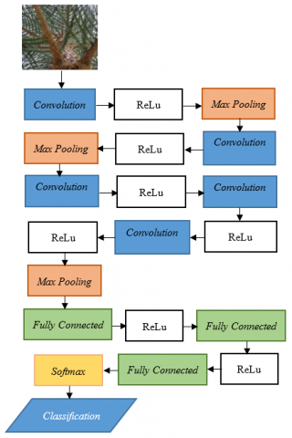
3.2 Needle-leaf type AlexNet architecture
AlexNet is a CNN architecture consisting of eight feature extraction layers [24]. The AlexNet model on the needle leaf type image can be seen in Figure 2.
Figure 2. Needle-leaf type AlexNet architecture
The experiment in this research uses an input image measuring 224 x 224 pixels with three color channels, namely Red, Green, and Blue. Eight feature extraction layers follow this stage. These layers are divided into five convolution layers and three pooling layers. The pooling layer used is max polling. In its classification layer, AlexNet has two Fully Connected layers, each consisting of 4096 neurons. At this layer's end is a classification process using softmax activation [25].
3.3 Needle leaf type VGG16 architecture
The VGG16 CNN model consists of a total of 13 convolution layers, five pooling layers, three fully-connected layers, and one output layer [26]. The VGG16 model on the needle leaf type image can be seen in Figure 3.
In this experiment, the VGG16 model processes an input layer with a 224 x 224 pixels resolution and three color channels (RGB). This process is followed by 13 convolution layers, where the ReLU activation function is used after each convolution operation. Additionally, several max-pooling layers are applied to convolution layers using 2x2 filters. This aims to reduce the spatial dimensions of the needle leaf image while reducing the number of parameters required in the network. After going through a series of convolution layers and max pooling, the image's features are channeled into fully connected layers, each consisting of 4096 neurons. The final output layer consists of 1000 neurons, corresponding to the number of classes in the ImageNet dataset, which is generally used to train image recognition models. This output layer typically uses a softmax activation function to generate probabilities for each class.
Figure 3. Arsitektur VGG16 jenis daun jarum
3.4 AlexNet and VGG16 architectural accuracy against coniferous trees
3.4.1 Pinus merkusii
The AlexNet model achieved an accuracy rate of 98% on training data and 86.00% for validation data in classifying the density and transparency classes of Merkusii pine trees when using a Tesla K80 GPU machine in 2510 seconds. On the other hand, the change in loss value in the AlexNet model for density and transparency classification in Merkusii pine trees was around 0.24% on the training data. In contrast, on the validation data, it reached approximately 68.89%. Meanwhile, the VGG16 model achieved an accuracy level of 100% on training data. In comparison, on validation data, it gained 90.00% in classifying the density and transparency classes of Merkusii pine trees when treated with a Tesla K80 GPU engine, and this was achieved in 110.00 seconds. On the other hand, the change in loss value in the VGG16 model for density and transparency classification in Merkusii pine trees was around 2.11% on the training data. On the validation data, it reached approximately 34.63%.
3.4.2 Araucaria heterophylla
The AlexNet model achieved an accuracy level of 100% on training data and 87.00% for validation data in classifying density and transparency classes of Araucaria heterophylla trees when using a TeslaK80 GPU in 2285 seconds. On the other hand, the change in loss value in the AlexNet model for density and transparency classification in Merkusii pine trees was around 0.0070% on the training data. In contrast, on the validation data, it reached approximately 52.78%. Meanwhile, the VGG16 model for classifying Araucaria heterophylla trees in determining density and transparency classes, when run using a Tesla K80 GPU, achieved an accuracy level of 100% on training data. In comparison, data validation attained an accuracy of 92.00% in 85.00 seconds. Changes in the loss value in the model decreased, but the loss value was almost stable. The final value of loss on training data is around 0.89%, while it reaches approximately 21.86% on validation data.
3.4.3 Cupressus retusa
The AlexNet model achieved an accuracy level of 100% on training data and 96.00% for validation data in classifying the density and transparency classes of cupressus retusa trees when using a Tesla K80 GPU machine within seconds. On the other hand, the change in loss value in the AlexNet model for density and transparency classification in the Cupressus retusa tree was around 6.49% on the training data. In contrast, on the validation data, it reached approximately 37.54%. Meanwhile, the VGG16 architectural model applied to the density and transparency classification of Cupressus retusa trees, when run using a Tesla K80 GPU, achieved an accuracy level of 100% on the training data. In comparison, the validation data achieved an accuracy of around 96.00% in 95.00 seconds. The loss value in the model decreased but was not stable. The final loss value on the training data was about 1.18%, while it reached around 12.83% on the validation data.
3.4.4 Shorea javanica
The AlexNet model achieved an accuracy level of 100% on training data and 95.00% for validation data in classifying the density and transparency classes of Shorea javanica trees when using a Tesla K80 GPU in 2376 seconds. On the other hand, the change in the loss value in the AlexNet model for density and transparency classification in the Shorea javanica tree is around 0.0013% on the training data. In contrast, on the validation data, it reaches approximately 0.25%. Meanwhile, the VGG16 model applied to density and transparency classification on shorea javanica trees, when run using a Tesla K80 GPU, succeeded in achieving an accuracy level of 100% on the training data. In comparison, data validation attained an accuracy of around 99.00% in 100.00 seconds. The loss value in the model decreases inconsistently. The final value of a loss on training data is approximately 0.11%, while it reaches around 2.35% on validation data.
3.5 Confusion matrix of coniferous trees
The confusion matrix includes model evaluation on images of coniferous trees based on density and transparency classes of conifers.
3.5.1 Pinus merkusii
Table 3 shows the results of testing the AlexNet architecture on the Mersusii pine tree type on a Tesla K80 GPU computer. False positive (FP) value, namely, the model incorrectly predicts an image into a class. In a class with a density of 15, there are 5 FPs, which means 2 images are actually a density class of 5 and 3 images are actually a density class of 35. Likewise, in a class with a density of 25, there are 3 FPs, which means one image of them is actually a density of 5, and two images are actually a density of 95. A similar thing happens in the class with a density of 35, where there are 5 FPs, one of the images is actually a density of 5, 2 images are actually a density of 15, and 1 image is actually a density of 85. Likewise, in a class with a density of 45, there are 8 FPs, which means three images actually have a density of 5, two images actually have a density of 55, one image actually has a density class of 65, and two images actually have a density class of 75. Similar patterns also occur in other classes.
Apart from FP, there is also a false negative (FN) value, namely a false negative prediction. The model fails to identify something that should belong to a class. From the test results, there were 8 false negatives at a density of 5, which means the model failed to identify 8 images that should belong to a certain class. Of the 8 images, 2 images were incorrectly predicted as density 15, 1 image was incorrectly predicted as density 25, 1 image was incorrectly predicted as density 35, 3 images were incorrectly predicted as density 45, and 1 image was incorrectly predicted as density 85. At density 15, there were 3 FNs, where 2 images were incorrectly predicted as density 35 and 1 image was incorrectly predicted as density 55. At density 25, there were 2 FNs, of which 2 images were incorrectly predicted as density 75. At density 35 with 5 FNs, where 3 images were incorrectly predicted as density 15 and 2 images were incorrectly predicted as density 55). At a density of 55, there are 2 FNs, where 2 images are incorrectly predicted as having a density 45. At a density of 65, there is 1 FN, where there is 1 image that is incorrectly predicted as having a density 45. At density 75, there are 2 FNs, which means 2 images are incorrectly predicted as density 45. At a density of 85, there is 1 FN, where 1 image is incorrectly predicted to have a density of 35. At a density of 95 with 4 FNs, where 2 images are incorrectly predicted as a density of 25 and 2 images are incorrectly predicted as a density of 75.
From the results of testing the AlexNet architecture on the Merkusii pine tree species, a number of false positive (FP) and false negative (FN) values were found, which describe the model's performance in predicting density classes. The model often incorrectly classifies images into inappropriate classes. This is indicated by the presence of FP values and similar patterns in other density and transparency classes. This analysis of model accuracy from FP and FN values shows that there is room for improvement in model performance. With incorrect predictions for both FP and FN, the model is less accurate in identifying density and transparency classes in the Merkusii pine tree species.
Table 3. Confusion matrix AlexNet pinus merkusii
|
Original Class |
Prediction Result Class |
|||||||||
|
CD5, FT95 |
CD15, FT85 |
CD25, FT75 |
CD35, FT65 |
CD45, FT55 |
CD55, FT45 |
CD65, FT35 |
CD75, FT25 |
CD85, FT15 |
CD95, FT5 |
|
|
CD5, FT95 |
17 |
2 |
1 |
1 |
3 |
0 |
0 |
0 |
1 |
0 |
|
CD15, FT85 |
0 |
12 |
0 |
2 |
0 |
1 |
0 |
0 |
0 |
0 |
|
CD25, FT75 |
0 |
0 |
25 |
0 |
0 |
0 |
0 |
2 |
0 |
0 |
|
CD35, FT65 |
0 |
3 |
0 |
19 |
0 |
2 |
0 |
0 |
0 |
0 |
|
CD45, FT55 |
0 |
0 |
0 |
0 |
14 |
0 |
0 |
0 |
0 |
0 |
|
CD55, FT45 |
0 |
0 |
0 |
0 |
2 |
19 |
0 |
0 |
0 |
0 |
|
CD65, FT35 |
0 |
0 |
0 |
0 |
1 |
0 |
20 |
0 |
0 |
0 |
|
CD75, FT25 |
0 |
0 |
0 |
0 |
2 |
0 |
0 |
9 |
0 |
0 |
|
CD85, FT15 |
0 |
0 |
0 |
1 |
0 |
0 |
0 |
0 |
20 |
0 |
|
CD95, FT5 |
0 |
0 |
2 |
0 |
0 |
0 |
0 |
2 |
0 |
17 |
Table 4. Confusion matrix VGG16 pinus merkusii
|
Original Class |
Prediction Result Class |
|||||||||
|
CD5, FT95 |
CD15, FT85 |
CD25, FT75 |
CD35, FT65 |
CD45, FT55 |
CD55, FT45 |
CD65, FT35 |
CD75, FT25 |
CD85, FT15 |
CD95, FT5 |
|
|
CD5, FT95 |
21 |
2 |
0 |
2 |
0 |
0 |
0 |
0 |
0 |
0 |
|
CD15, FT85 |
0 |
13 |
0 |
2 |
0 |
0 |
0 |
0 |
0 |
0 |
|
CD25, FT75 |
0 |
0 |
26 |
0 |
0 |
0 |
0 |
0 |
0 |
1 |
|
CD35, FT65 |
0 |
2 |
0 |
22 |
0 |
0 |
0 |
0 |
0 |
0 |
|
CD45, FT55 |
0 |
0 |
0 |
0 |
14 |
0 |
0 |
0 |
0 |
0 |
|
CD55, FT45 |
0 |
0 |
0 |
0 |
0 |
20 |
1 |
0 |
0 |
0 |
|
CD65, FT35 |
0 |
1 |
0 |
1 |
0 |
0 |
19 |
0 |
0 |
0 |
|
CD75, FT25 |
0 |
0 |
0 |
0 |
0 |
0 |
0 |
11 |
0 |
0 |
|
CD85, FT15 |
0 |
0 |
0 |
1 |
0 |
0 |
1 |
0 |
19 |
0 |
|
CD95, FT5 |
0 |
0 |
3 |
0 |
0 |
0 |
0 |
2 |
0 |
16 |
Table 5. Confusion matrix AlexNet araucaria heterophylla
|
Original Class |
Prediction Result Class |
|||||||||
|
CD5, FT95 |
CD15, FT85 |
CD25, FT75 |
CD35, FT65 |
CD45, FT55 |
CD55, FT45 |
CD65, FT35 |
CD75, FT25 |
CD85, FT15 |
CD95, FT5 |
|
|
CD5, FT95 |
21 |
0 |
0 |
0 |
0 |
3 |
0 |
0 |
1 |
0 |
|
CD15, FT85 |
1 |
12 |
0 |
0 |
0 |
2 |
0 |
0 |
0 |
0 |
|
CD25, FT75 |
1 |
0 |
26 |
0 |
0 |
0 |
0 |
2 |
0 |
0 |
|
CD35, FT65 |
0 |
0 |
0 |
24 |
0 |
0 |
0 |
0 |
0 |
0 |
|
CD45, FT55 |
0 |
0 |
0 |
0 |
14 |
0 |
0 |
0 |
0 |
0 |
|
CD55, FT45 |
2 |
0 |
0 |
0 |
0 |
17 |
1 |
0 |
1 |
0 |
|
CD65, FT35 |
0 |
0 |
1 |
0 |
0 |
1 |
19 |
0 |
1 |
0 |
|
CD75, FT25 |
0 |
0 |
0 |
0 |
0 |
0 |
0 |
11 |
0 |
0 |
|
CD85, FT15 |
0 |
0 |
0 |
0 |
0 |
0 |
0 |
0 |
21 |
0 |
|
CD95, FT5 |
0 |
0 |
0 |
0 |
0 |
0 |
0 |
0 |
0 |
21 |
Table 6. Confusion matrix VGG16 araucaria heterophylla
|
Original Class |
Prediction Result Class |
|||||||||
|
CD5, FT95 |
CD15, FT85 |
CD25, FT75 |
CD35, FT65 |
CD45, FT55 |
CD55, FT45 |
CD65, FT35 |
CD75, FT25 |
CD85, FT15 |
CD95, FT5 |
|
|
CD5, FT95 |
25 |
0 |
0 |
0 |
0 |
0 |
0 |
0 |
0 |
0 |
|
CD15, FT85 |
0 |
11 |
0 |
1 |
0 |
2 |
0 |
0 |
1 |
0 |
|
CD25, FT75 |
1 |
0 |
26 |
0 |
0 |
0 |
0 |
0 |
0 |
0 |
|
CD35, FT65 |
0 |
0 |
0 |
24 |
0 |
0 |
0 |
0 |
0 |
0 |
|
CD45, FT55 |
0 |
0 |
0 |
0 |
14 |
0 |
0 |
0 |
0 |
0 |
|
CD55, FT45 |
0 |
4 |
0 |
0 |
0 |
14 |
0 |
0 |
3 |
0 |
|
CD65, FT35 |
0 |
2 |
0 |
0 |
0 |
0 |
19 |
0 |
0 |
0 |
|
CD75, FT25 |
0 |
0 |
0 |
0 |
0 |
0 |
0 |
11 |
0 |
0 |
|
CD85, FT15 |
1 |
0 |
0 |
0 |
0 |
0 |
0 |
0 |
20 |
0 |
|
CD95, FT5 |
0 |
0 |
0 |
0 |
0 |
0 |
0 |
0 |
0 |
21 |
Table 4 shows the confusion matrix results of the VGG16 architecture on the Merkusii pine tree on a Tesla K80 GPU machine. The FP and FN values must be lowered to improve model performance so that it can predict the class density and canopy transparency of Merkusii pine trees more precisely. There is an FP (false positives) value in density class 15, with 5 images actually in density class 35, 1 image actually in density class 65, and 2 images actually in density class 5. Then, in density class 25, there are actually 3 images in density class 95. In density class 35, there are 6 FPs consisting of 2 real images of density class 5, 2 real images of density class 15, 1 real image of density class 65, and 1 real image of density class 85. Density class 65 has 2 FPs, with 1 real image of density class 55 and 1 image that is actually density class 85. Finally, density class 75 has two images that are actually density class 95.
FN (false negatives) also occurs in some classes. In density class 5, there are 4 FNs consisting of 2 images incorrectly predicted as density 15 and 2 images incorrectly predicted as density 35. In density class 15, there are 2 FNs, which means 2 images are incorrectly predicted as density 35. In density class 25, there is 1; the image was incorrectly predicted as density 95. In density class 35, there were 2 images incorrectly predicted as density 15. In the density class 55, there was one image incorrectly predicted as having a density 65. In the density class 65, there were 2 FNs, with 1 image incorrectly predicted as density 15 and 1 image incorrectly predicted as density 35. At density class 85, there are 2 FNs, with 1 image incorrectly predicted as density 35 and 1 image incorrectly predicted as density 65. Finally, at density 95, there are 5 FNs, with three images incorrectly predicted as density 25 and two images incorrectly predicted as density 75.
From the results of testing the VGG16 architecture on the merkusii pine tree species, a number of false positive (FP) and false negative (FN) values can be seen, which reflect the model's performance in predicting density classes. The model often experiences errors in assigning images to inappropriate classes, which is reflected in the presence of FP values and similar patterns in other density and transparency classes. Evaluation of model accuracy based on FP and FN values shows that there is room to improve model performance. With inaccurate predictions for both FP and FN, the model is less accurate in recognizing density and transparency classes in the Merkusii pine tree species.
3.5.2 Araucaria heterophylla
Table 5 shows the results of the AlexNet architecture confusion matrix for the Araucaria heterophylla tree on the K80 GPU machine. False positive (FP) values in several classes, such as density class 5 with 4 FP, where one image is actually density class 15, one image is actually density class 25, and one image is actually density class 55. In density class 25, there is one image that is actually density class 65. Density class 55 has 6 FPs, which means three images are actually of density class 5, two images are actually of density class 15, and one image is actually of density class 65. At density 65, there is actually 1 image of density class 55. At density 75, there are actually 2 images of density class 25. Density class 85 with 3 FP, which means one image is actually density class 5, one image is actually density class 55, and one image is actually density class 65. False negative (FN) values are also seen in density class 5 with 4 FN, where 3 images are incorrectly predicted as density 55 and 1 image is incorrectly predicted as density 85. Density 15 with 3 FN, where 1 image is incorrectly predicted as density 5, and 2 images are incorrectly predicted as density 55. Density 25 with 3 FN, where 1 image is incorrectly predicted as density 5, and 2 images are incorrectly predicted as density 75. Density 55 with 4 FN, where 2 images are incorrectly predicted as density 5, 1 image is incorrectly predicted as density 65, and 1 image is incorrectly predicted as density 85. At density 65, there are 3 FNs, of which 1 image is incorrectly predicted as density 25, 1 image is incorrectly predicted as density 55, and 1 image is incorrectly predicted as density 85.
From the results of testing the AlexNet architecture on the Araucaria heterophylla tree species, there are a number of false positive (FP) and false negative (FN) values that reflect the model's performance in predicting density classes. The model often makes mistakes in placing images into inappropriate classes, which can be seen from the FP values and similar patterns in other density and transparency classes. Assessment of model accuracy based on FP and FN values shows that there is room to improve model performance. With inaccurate predictions for both FP and FN, the model becomes less precise in recognizing density and transparency classes in the Araucaria heterophylla tree species.
Table 6 shows the results of the VGG16 architecture matrix confusion on Araucaria heterophylla trees on a Tesla K80 GPU machine. FP (false positives) values are found in several classes, such as density class 5 with 2 FP, where one image is actually density class 25 and one image is actually density class 85. In density class 15 with 6 FP, four images are actually density class 55 and two are actual images of density class 65. For density class 35, there is 1 FP, which marks one true image of density class 15, density class 55 with 2 FP, which marks 2 true images of density class 15, and density class 85 with 4 FP, where one image is actually density class 15 and 3 images are actually density class 55. Meanwhile, FNs (false negatives) are also found in several classes, such as density class 15 with 4 FNs, where 1 image is incorrectly predicted as density 35, 2 images are incorrectly predicted as density 55, and 1 image is incorrectly predicted as density 85. For the density class 25 with 1 FN, there is 1 image incorrectly predicted as density 5. For the density class 55 with 7 FN, there are 4 images incorrectly predicted as density 15 and 3 images incorrectly predicted as density 85. For density class 65, there are 2 images incorrectly predicted as density 15. In density class 65 with 2 FN, 1 image is incorrectly predicted as density 15, and 1 image is incorrectly predicted as density 35. And density class 85, with 1 image incorrectly predicted as density 5.
From the results of testing the VGG16 architecture on the Araucaria heterophylla tree species, there are several false positive (FP) and false negative (FN) values that reflect the model's performance in predicting density classes. The model often makes mistakes in placing images into inappropriate classes, which can be seen from the presence of FP and similar patterns in other density and transparency classes. Evaluation of model accuracy based on FP and FN values shows that there is room to improve model performance. With inaccurate predictions for both FP and FN, the model becomes less effective in recognizing density and transparency classes in the Araucaria heterophylla tree species.
3.5.3 Cupressus retusa
Table 7 shows the confusion matrix results of the AlexNet architecture for the Cupressus Retusa tree on a Tesla K80 GPU machine. In several classes, such as density class 5, there are 3 false positive (FP) values, which means 3 images are actually density class 85. At density 15, there is 1 FP, which means 1 image is actually density class 5. At density 45, there is 1 real image density class 5. For density 55 with 1 FP, which means 1 image is actually density class 65, At density 65 with 4 FP, where 4 images are actually density class 55. For density class 75 with 3 FP, there are actually two images of density class 25, and one image is actually density class 95. Meanwhile, density is 85 with 3 FP, which means 3 images are actually density class 5. False negative (FN) values are also seen in density class 5 with 5 FN, where 1 image is incorrectly predicted as density 15, 1 image is incorrectly predicted as density 45, and 3 images are incorrectly predicted as density 85. At density 25 with 2 FN, which means 2 images are incorrectly predicted as density 75. For density 55 with 4 FN, 4 images are incorrectly predicted as density 65. At density 65 with 2 FN, where 1 image is incorrectly predicted as density 5 and 1 image is incorrectly predicted as density 55. Meanwhile, density 85 with 3 FN, where 3 images are incorrectly predicted as density 5.
From the results of testing the AlexNet architecture on the Cupressus retusa tree species, a number of false positive (FP) and false negative (FN) values can be seen, which describe the model's performance in predicting density classes. The model often incorrectly assigns images to inappropriate classes, as seen by the FP values and similar patterns in other density and transparency classes. Evaluation of model accuracy based on FP and FN values shows that there is room to improve model performance. With less accurate predictions, both FP and FN, the model becomes less effective in recognizing density and transparency classes in the Cupressus retusa tree species.
Table 8 shows the confusion matrix results of the VGG16 architecture on the Cupressus Retusa tree on a Tesla K80 GPU machine. There are FP (false positives) values in several classes, such as density class 5 with 2 FP, which means 2 images are actually a density of 85. For density class 25 with 2 FP, which means 2 images are actually a density of 5, For density class 35 with 1 FP, which means 1 image is actually a density of 15, In the density class 75, there is 1 FP, which means 1 image is actually a density of 95. Meanwhile, the density class 85 has 4 FPs, which means three images are actually a density of 5, and one image is actually a density of 65. On the other hand, there are also FN (false negatives) in several classes, such as density class 5 with 5 FN, which means 2 images were incorrectly predicted as density 25, and 3 images were incorrectly predicted as density 85. For density class 25 with 2 FN, which means 2 images incorrectly predicted as density 75, For density class 55 with 4 FN, which means 4 images were incorrectly predicted as density 65, For density class 65 with 1 FN, which means 1 image was incorrectly predicted as density 55. In density class 85 with 2 FN, which means 2 images were incorrectly predicted as density 5, Meanwhile, the density class is 95 with 1 FN, which means 1 image was incorrectly predicted as having a density 75.
From the test results using the VGG16 architecture on the Cupressus retusa tree species, there are a number of false positive (FP) and false negative (FN) values that indicate the model's performance in predicting density classes. The model rarely experiences errors in placing images into inappropriate classes, as evidenced by the existence of FP values and similar patterns in other density and transparency classes. Evaluation of model accuracy based on FP and FN values shows that there is room to improve model performance. With fairly accurate predictions for both FP and FN, the model can be considered quite effective in recognizing density and transparency classes in the Cupressus retusa tree species.
Table 7. Confusion matrix AlexNet cupressus retusa
|
Original Class |
Prediction Result Class |
|||||||||
|
CD5, FT95 |
CD15, FT85 |
CD25, FT75 |
CD35, FT65 |
CD45, FT55 |
CD55, FT45 |
CD65, FT35 |
CD75, FT25 |
CD85, FT15 |
CD95, FT5 |
|
|
CD5, FT95 |
20 |
0 |
2 |
0 |
0 |
0 |
0 |
0 |
3 |
0 |
|
CD15, FT85 |
0 |
14 |
0 |
1 |
0 |
0 |
0 |
0 |
0 |
0 |
|
CD25, FT75 |
0 |
0 |
27 |
0 |
0 |
0 |
0 |
0 |
0 |
0 |
|
CD35, FT65 |
0 |
0 |
0 |
24 |
0 |
0 |
0 |
0 |
0 |
0 |
|
CD45, FT55 |
0 |
0 |
0 |
0 |
14 |
0 |
0 |
0 |
0 |
0 |
|
CD55, FT45 |
0 |
0 |
0 |
0 |
0 |
21 |
0 |
0 |
0 |
0 |
|
CD65, FT35 |
0 |
0 |
0 |
0 |
0 |
0 |
20 |
0 |
1 |
0 |
|
CD75, FT25 |
0 |
0 |
0 |
0 |
0 |
0 |
0 |
11 |
0 |
0 |
|
CD85, FT15 |
2 |
0 |
0 |
0 |
0 |
0 |
0 |
0 |
19 |
0 |
|
CD95, FT5 |
0 |
0 |
0 |
0 |
0 |
0 |
0 |
1 |
0 |
20 |
Table 8. Confusion matrix VGG16 cupressus retusa
|
Original Class |
Prediction Result Class |
|||||||||
|
CD5, FT95 |
CD15, FT85 |
CD25, FT75 |
CD35, FT65 |
CD45, FT55 |
CD55, FT45 |
CD65, FT35 |
CD75, FT25 |
CD85, FT15 |
CD95, FT5 |
|
|
CD5, FT95 |
20 |
1 |
0 |
0 |
1 |
0 |
0 |
0 |
3 |
0 |
|
CD15, FT85 |
0 |
15 |
0 |
0 |
0 |
0 |
0 |
0 |
0 |
0 |
|
CD25, FT75 |
0 |
0 |
27 |
0 |
0 |
0 |
0 |
2 |
0 |
0 |
|
CD35, FT65 |
0 |
0 |
0 |
24 |
0 |
0 |
0 |
0 |
0 |
0 |
|
CD45, FT55 |
0 |
0 |
0 |
0 |
14 |
0 |
0 |
0 |
0 |
0 |
|
CD55, FT45 |
0 |
0 |
0 |
0 |
0 |
21 |
4 |
0 |
0 |
0 |
|
CD65, FT35 |
1 |
0 |
0 |
0 |
0 |
1 |
19 |
0 |
0 |
0 |
|
CD75, FT25 |
0 |
0 |
0 |
0 |
0 |
0 |
0 |
11 |
0 |
0 |
|
CD85, FT15 |
2 |
0 |
0 |
0 |
0 |
0 |
0 |
0 |
19 |
0 |
|
CD95, FT5 |
0 |
0 |
0 |
0 |
0 |
0 |
0 |
1 |
0 |
20 |
Table 9. Confusion matrix AlexNet shorea javanica
|
Original Class |
Prediction Result Class |
|||||||||
|
CD5, FT95 |
CD15, FT85 |
CD25, FT75 |
CD35, FT65 |
CD45, FT55 |
CD55, FT45 |
CD65, FT35 |
CD75, FT25 |
CD85, FT15 |
CD95, FT5 |
|
|
CD5, FT95 |
25 |
0 |
0 |
0 |
0 |
0 |
0 |
0 |
0 |
0 |
|
CD15, FT85 |
0 |
15 |
0 |
0 |
0 |
0 |
0 |
0 |
0 |
0 |
|
CD25, FT75 |
0 |
0 |
27 |
0 |
0 |
0 |
0 |
0 |
0 |
0 |
|
CD35, FT65 |
0 |
1 |
0 |
20 |
0 |
2 |
0 |
1 |
0 |
0 |
|
CD45, FT55 |
0 |
0 |
0 |
0 |
14 |
0 |
0 |
0 |
0 |
0 |
|
CD55, FT45 |
0 |
0 |
0 |
1 |
0 |
19 |
1 |
0 |
0 |
0 |
|
CD65, FT35 |
0 |
0 |
0 |
1 |
0 |
0 |
20 |
0 |
0 |
0 |
|
CD75, FT25 |
0 |
0 |
2 |
0 |
0 |
0 |
0 |
9 |
0 |
0 |
|
CD85, FT15 |
0 |
0 |
0 |
0 |
0 |
0 |
0 |
0 |
21 |
0 |
|
CD95, FT5 |
0 |
0 |
1 |
0 |
0 |
0 |
0 |
0 |
0 |
20 |
Table 10. Confusion matrix VGG16 shorea javanica
|
Original Class |
Prediction Result Class |
|||||||||
|
CD5, FT95 |
CD15, FT85 |
CD25, FT75 |
CD35, FT65 |
CD45, FT55 |
CD55, FT45 |
CD65, FT35 |
CD75, FT25 |
CD85, FT15 |
CD95, FT5 |
|
|
CD5, FT95 |
25 |
0 |
0 |
0 |
0 |
0 |
0 |
0 |
0 |
0 |
|
CD15, FT85 |
0 |
15 |
0 |
0 |
0 |
0 |
0 |
0 |
0 |
0 |
|
CD25, FT75 |
0 |
0 |
27 |
0 |
0 |
0 |
0 |
0 |
0 |
0 |
|
CD35, FT65 |
0 |
0 |
0 |
24 |
0 |
0 |
0 |
0 |
0 |
0 |
|
CD45, FT55 |
0 |
0 |
0 |
0 |
14 |
0 |
0 |
0 |
0 |
0 |
|
CD55, FT45 |
0 |
0 |
0 |
0 |
0 |
21 |
0 |
0 |
0 |
0 |
|
CD65, FT35 |
0 |
0 |
0 |
0 |
0 |
0 |
21 |
0 |
0 |
0 |
|
CD75, FT25 |
0 |
0 |
0 |
0 |
0 |
0 |
0 |
11 |
0 |
0 |
|
CD85, FT15 |
0 |
0 |
0 |
0 |
0 |
0 |
0 |
0 |
21 |
0 |
|
CD95, FT5 |
0 |
0 |
1 |
0 |
0 |
0 |
0 |
0 |
0 |
20 |
3.5.4 Shorea javanica
Table 9 shows the confusion matrix results of the AlexNet architecture for the Shorea Javanica tree on the K80 GPU machine. False positive (FP) values in several classes, for example, density class 15 with 1 FP, means 1 image is actually density 35. Density class 25 with 3 FP, which means 3 images are actually density 75 and one image is actually density 95. For density class 35 with 2 FP, which means 2 images are actually a density of 55 and one image is actually a density of 65, Density 55 with 2 FP, which means 2 images are actually a density of 35. Density 65 with 1 FP, where 1 image is actually a density of 55. Density 75 with 1 FP, meaning that 1 image is actually a density of 35. False negative (FN) values are also seen in the density class 35 with 4 FNs, where 1 image is incorrectly predicted as a density of 15, 2 images are incorrectly predicted as a density of 55, and 1 image is incorrectly predicted as a density of 75. Density 55 with 2 FN, where 1 image is incorrectly predicted as density 35 and 1 image is incorrectly predicted as density 65. Density 65 with 1 FN, where 1 image is incorrectly predicted as density 35. Meanwhile, density class 75 with 2 FN, which is 2 images wrongly predicted as a density of 25, Meanwhile, the density class is 95 with 1 FN, where 1 image is wrongly predicted as a density of 25.
Based on test results using the AlexNet architecture on the Shorea javanica tree species, there are a number of false positive (FP) and false negative (FN) values that indicate the model's performance in predicting density classes. The model often experiences errors in placing images into inappropriate classes, as evidenced by the existence of FP values and similar patterns in other density and transparency classes. Evaluation of model accuracy based on FP and FN values shows that there is room to improve model performance. With less accurate predictions, both FP and FN, the model can be considered less effective in recognizing density and transparency classes in the Shorea javanica tree species.
Table 10 depicts the confusion matrix results for the VGG16 architecture on Shorea javanica trees. However, FP and FN still appear in the performance of the VGG16 model on shorea javanica trees, which were evaluated using the Tesla K80 GPU engine. One case of FP can be observed in density class 25, where one image is actually density 95. In addition, one case of FN was found in density class 95, where one image was incorrectly predicted as density 25.
Based on test results using the VGG16 architecture on the Shorea javanica tree species, there is one false positive (FP) and one false negative (FN) value, which indicates the model's performance in predicting density and transparency classes. The model almost does not experience errors in placing images into inappropriate classes, as evidenced by the presence of 1 FP and FN values. With accurate predictions in both FP and FN, the model can be considered effective in recognizing density and transparency classes in the Shorea javica tree species.
3.6 Performance comparison between AlexNet and VGG16
The following are the differences between AlexNet and VGG16.
The differences in the AlexNet and VGG architectures can be seen in Table 11. AlexNet uses hyperparameters as in Table 11. These hyperparameters were after carrying out several experiments during the research to get the best accuracy from the AlexNet and VGG16 models. AlexNet also has 11 layers, consisting of 5 convolutional layers, 3 max pooling, and 3 fully connected layers while VGG16 is much deeper with a total of 21 layers, including 13 convolutional layers, 5 max pooling, and 3 fully connected layers. AlexNet uses a 'wide' configuration with the addition of larger layers in proportion to depth, for example 96, 256, 384, and 384 filters in the convolution layer. VGG16 uses a 'deep' configuration with all convolution layers having a relatively small number of filters (64 or 128) but a deeper structure. VGG16 learns images more deeply and has more parameters so it is typically slower to train than AlexNet. VGG16 often provides better results in object recognition tasks due to its greater depth and complexity. However, AlexNet has introduced important concepts such as dropout, which influenced subsequent convolutional neural network architecture designs. In this study, the VGG16 results were better than AlexNet because the VGG16 model learned more deeply about the images used and the hyperparameters used as in Table 11.
Table 11. Comparison of AlexNet and VGG16
|
Arsitektur |
Hyperparameter |
Layer |
|
AlexNet |
Epoch 20 |
11 |
|
Batch-size 8 |
||
|
Learning-rate 0.0001 |
||
|
VGG16 |
Epoch 10 |
21 |
|
Batch-size 32 |
||
|
Learning-rate 0.001 |
In this research, introducing density levels and editorial transparency using four variations of needle leaves has been successfully implemented using the AlexNet and VGG16 architecture. The AexNet architecture model in identifying the level of density and transparency in needle leaves on the Tesla K80 machine produces an accuracy for the Araucaria heterophylla needle leaf type of 93.00%. In comparison, for Shorea javanica it reaches 99.00%. Meanwhile, this model also achieved an accuracy of 96.00% for Cupressus retusa and 86.00% for Pinus merkusii. Meanwhile, the accuracy results obtained by the VGG16 architecture when using the Tesla K80 machine to identify density and transparency in Pinus merkusii needle leaves were around 90.00%. In contrast, in Araucaria heterophylla needle leaves, it reached around 92.00%. For Cupressus retusa needle leaves, this architecture achieves an accuracy of approximately 96.00%; for Shorea javanica needle leaves, the accuracy even reaches around 99.00%.
The AlexNet model experienced errors in classifying or predicting 20 images of Araucaria heterophylla trees, 10 images of Cupressus retusa, 28 images of Pinus merkusii, and four images of Shorea javanica. Meanwhile, errors in classifying images in the VGG16 architecture included 19 images of Pinus merkusii trees, 15 images of Araucaria heterophylla trees, 10 images of Cupressus retusa trees, and one image of Shorea javanica trees. This error occurs because there are similar patterns and positions in the image.
In the research, it is necessary to add pictures of types of needle leaves with more and more variations for each class. This will help increase the level of accuracy of the resulting model. It is important to review hyperparameter settings and, if possible, measure these values greater than those used in this study. This can help achieve a higher level of accuracy in the model. In addition to the AlexNet and VGG16 architectures, you should consider using other Convolutional Neural Network (CNN) architectures such as LeNet, MobileNet, EfficientNet, etc. This will help compare accuracy results between various architectures so you can choose the one that provides optimal results. This research can also be further developed by integrating it into a website or mobile-based application. This will make it easier to monitor and use the model for various practical purposes. This research will be applied in the forestry sector, especially for monitoring forest health in the Wan Abdul Rachman Community Forest Park, Lampung, Indonesia.
[1] Pranolo, A., Widyastuti, S.M. (2014). Simple additive weighting method on intelligent agent for urban forest health monitoring. In 2014 International Conference on Computer, Control, Informatics and Its Applications (IC3INA), Bandung, Indonesia, pp. 132-135. https://doi.org/10.1109/IC3INA.2014.7042614
[2] Ansori, D.P., Safe’i, R., Kaskoyo, H. (2020). Penilaian indikator kesehatan hutan rakyat pada beberapa pola tanam (Studi kasus di Desa Buana Sakti, Kecamatan Batang Hari, Kabupaten Lampung Timur). Jurnal Perennial, 16(1): 1-6. https://doi.org/10.24259/perennial.v16i1.8109
[3] Safe’i, R., Darmawan, A., Kaskoyo, H., Rezinda, C.F.G. (2021). Analysis of changes in forest health status values in conservation forest (Case study: Plant and animal collection blocks in wan abdul rachman forest park (tahura war)). In Journal of Physics: Conference Series 1842(1): 012049. https://doi.org/10.1088/1742-6596/1842/1/012049
[4] Lausch, A., Borg, E., Bumberger, J., Dietrich, P., Heurich, M., Huth, A., Schaepman, M.E. (2018). Understanding forest health with remote sensing, part III: requirements for a scalable multi-source forest health monitoring network based on data science approaches. Remote Sensing, 10(7): 1120. https://doi.org/10.3390/rs10071120
[5] Arwanda, E.R., Safe’i, R. (2021). Assessment of forest health status of panca indah lestari community plantation forest (case study in bukit layang village, bakam district, bangka regency, bangka belitung province). In IOP Conference Series: Earth and Environmental Science, 918(1): 012031. https://doi.org/10.1088/1755-1315/918/1/012031
[6] Mangold, R.D. (2000). Overview of the forest health monitoring program. United States Department of Agriculture Forest Service General Technical Report NC, 129-140.
[7] Zhang, L., Xia, G.S., Wu, T., Lin, L., Tai, X.C. (2016). Deep learning for remote sensing image understanding. Journal of Sensors, 2016: 7954154. https://doi.org/10.1155/2016/7954154
[8] Sun, Y., Liu, Y., Zhou, H., Hu, H. (2021). Plant diseases identification through a discount momentum optimizer in deep learning. Applied Sciences, 11(20): 9468. https://doi.org/10.3390/app11209468
[9] Aradea, A., Rianto, R., Mubarok, H., Darmawan, I. (2023). Deep learning-based regional plant type recommendation system for enhancing agricultural productivity. Ingénierie des Systèmes d'Information, 28(4): 853-859. https://doi.org/10.18280/isi.280406
[10] Gonzalez, T.F. (2007). Handbook of approximation algorithms and metaheuristics. Chapman and Hall/CRC. p. 1432. https://doi.org/10.1201/9781420010749
[11] Narvekar, C., Rao, M. (2020). Flower classification using CNN and transfer learning in CNN-Agriculture Perspective. In 2020 3rd International Conference on Intelligent Sustainable Systems (ICISS), Thoothukudi, India, pp. 660-664. https://doi.org/10.1109/ICISS49785.2020.9316030
[12] Borugadda, P., Lakshmi, R., Govindu, S. (2021). Classification of cotton leaf diseases using AlexNet and machine learning models. Current Journal of Applied Science and Technology, 40(38): 29-37. https://doi.org/10.9734/cjast/2021/v40i3831588
[13] Tang, S., Yuan, S., Zhu, Y. (2020). Data preprocessing techniques in convolutional neural network based on fault diagnosis towards rotating machinery. IEEE Access, 8: 149487-149496. https://doi.org/10.1109/ACCESS.2020.3012182
[14] Thayumanasamy, I., Ramamurthy, K. (2022). Performance analysis of machine learning and deep learning models for classification of Alzheimer’s disease from brain MRI. Traitement du Signal, 39(6): 1961-1970. https://doi.org/10.18280/ts.390608
[15] Alzubaidi, L., Zhang, J., Humaidi, A.J., Al-Dujaili, A., Duan, Y., Al-Shamma, O., Farhan, L. (2021). Review of deep learning: concepts, CNN architectures, challenges, applications, future directions. Journal of Big Data, 8: 1-74. https://doi.org/10.1186/s40537-021-00444-8
[16] Maxwell, A.E., Warner, T.A., Guillén, L.A. (2021). Accuracy assessment in convolutional neural network-based deep learning remote sensing studies-Part 1: Literature review. Remote Sensing, 13(13): 2450. https://doi.org/10.3390/rs13132450
[17] Tripathi, M. (2021). Analysis of convolutional neural network based image classification techniques. Journal of Innovative Image Processing (JIIP), 3(2): 100-117. https://doi.org/10.36548/jiip.2021.2.003
[18] Dhomne, A., Kumar, R., Bhan, V. (2018). Gender recognition through face using deep learning. Procedia Computer Science, 132: 2-10. https://doi.org/10.1016/j.procs.2018.05.053
[19] Andonie, R., Florea, A.C. (2020). Weighted random search for CNN hyperparameter optimization, International Journal of Computers Communications & Control, 15(2): 1-11. https://doi.org/10.15837/IJCCC.2020.2.3868
[20] Iwata, H., Hayashi, Y., Hasegawa, A., Terayama, K., Okuno, Y. (2022). Classification of scanning electron microscope images of pharmaceutical excipients using deep convolutional neural networks with transfer learning. International Journal of Pharmaceutics: X, 4: 100135. https://doi.org/10.1016/j.ijpx.2022.100135
[21] Fasounaki, M., Yüce, E.B., Öncül, S., İnce, G. (2021). CNN-based Text-independent automatic speaker identification using short utterances. In 2021 6th international conference on computer science and engineering (UBMK), Ankara, Turkey, pp. 413-418. https://doi.org/10.1109/UBMK52708.2021.9559031
[22] Sanjaya, J., Ayub, M. (2020). Augmentasi Data Pengenalan Citra Mobil Menggunakan Pendekatan Random Crop, Rotate, dan Mixup. Jurnal Teknik Informatika dan Sistem Informasi, 6(2): 311-323. https://doi.org/10.28932/jutisi.v6i2.2688
[23] Shorten, C., Khoshgoftaar, T.M. (2019). A survey on image data augmentation for deep learning. Journal of Big Data, 6(1): 1-48. https://doi.org/10.1186/s40537-019-0197-0
[24] Fu’Adah, Y.N., Wijayanto, I., Pratiwi, N.K.C., Taliningsih, F.F., Rizal, S., Pramudito, M.A. (2021). Automated classification of Alzheimer’s disease based on MRI image processing using convolutional neural network (CNN) with AlexNet architecture. In Journal of Physics: Conference Series, 1844(1): 012020. https://doi.org/10.1088/1742-6596/1844/1/012020
[25] Shanthi, T., Sabeenian, R.S. (2019). Modified AlexNet architecture for classification of diabetic retinopathy images. Computers & Electrical Engineering, 76: 56-64. https://doi.org/10.1016/j.compeleceng.2019.03.004
[26] Wang, H. (2020). Garbage recognition and classification system based on convolutional neural network vgg16. In 2020 3rd International Conference on Advanced Electronic Materials, Computers and Software Engineering (AEMCSE), Shenzhen, China, pp. 252-255. https://doi.org/10.1109/AEMCSE50948.2020.00061