Carol Praveen Raja Guy De Pongalan*![]() | Vetrimanikumar Jayaprakasham
| Vetrimanikumar Jayaprakasham![]() | Satya Srinivas Maddipati
| Satya Srinivas Maddipati![]() | Krishnakumar Selvaraj
| Krishnakumar Selvaraj![]()
© 2025 The authors. This article is published by IIETA and is licensed under the CC BY 4.0 license (http://creativecommons.org/licenses/by/4.0/).
OPEN ACCESS
Brain tumor detection and classification using computed tomography (CT) images is a major research field with the machine learning techniques and computer aided assessments. Computer and learning dependent image assessments improve the quality of diagnosis through early disease detection. However the conventional image processing techniques impose a feature selection problem to augment the quality improvements. Accuracy centric detections are less feasible due to improper or incomplete feature selection. To address this specific issue, Differential Feature Classification (DFC) is proposed in this article. This method strengthens the early detection process through precision feature selection. The features are classified based on false positives and true negative to reduce improper feature selection. The differential features are filtered using backpropagation learning for different new regions identified. The learning network is trained using the maximum differences estimated in heterogeneous regions. The regions with maximum differences are sorted out for identifying its associated features. The learning is further trained using the associated features to improve the detection precision. In this case, the true negatives and false positives are jointly used to improve the training rate of the learning network. Such process is recurrent until the final region is identified for detecting tumors. The proposed method is validated using real time CT image dataset and defined metrics to verify its efficiency. Thus, from the comparative analysis, the proposed method improves accuracy and precision by 9.33% and 9.84% respectively. The true negatives, false positives, and detection time are reduced by 11.67%, 11.95%, and 9.97% respectively.
back propagation learning, brain tumor, CT image, feature extraction, region differentiation
Detecting brain tumors from Computed Tomography (CT) images poses a big challenge in the medical field. The fact that it is composed of different textures of brain tissues makes it hard to point out the difference between normal and tumorous tissue [1]. CT imaging, on the other hand, is mostly applied, with the use of advanced computational techniques, to capture the best possible picture of the brain [2]. Early detection of brain tumors is very critical as it avails timely intervention and treatment planning. So, refining the methods of detection will increase the accuracy and efficacy needed in the detection of brain tumors [3]. Despite the complexity, it means that the technology and methods employed in imaging and algorithms at work in this domain will continue to progress [4]. These underscore the necessity of research collaboration and specialization which is so important for the development of improved methods to diagnose brain tumors, leading to better patient outcomes [5].
Precision feature extraction and classification have become the objective of researchers engaged in developing methods to combat the challenges encountered in brain tumor detection in CT imaging [6]. By using image processing techniques, specific features that are indicative of tumor presence can be isolated and analyzed. These may include variations in tissue density, irregularities in shape, or anomalous textural patterns characteristic of a tumor [7]. Meticulous feature extraction and classification provide a more accurate separation between healthy brain tissue and the regions that are affected by the tumor [8]. So, the precision in feature analysis is highly essential for minimizing false positives, and ensuring reliable detection of brain tumors, leading to timely intervention and reduced impact on patients [9]. This means that such efforts and ongoing research in improving feature extraction algorithms and classification techniques are imperative in enhancing brain tumor detection accuracy [10].
Machine learning algorithms have recently greatly improved the detection of brain tumors from CT images [11]. Examining features and aiding in decision-making identifies tumor-specific patterns through machine-learning techniques has automated and streamlined the process of pattern identification [12]. Feature selection techniques like back-propagation learning are applied to train models on labeled datasets, allowing them to discern subtle variations in features representing tumor presence [13]. Iterative learning and refinement of these models allow for refinement and optimization of the feature classification criteria [14]. These combinations further strengthen the enhancements in the way feature classification works in improving detection accuracy, with the added benefit of scalability and applicability across myriad patient populations and imaging modalities [15]. Such a perspective thus stresses the need to continuously research the machine learning algorithms, often integrated to better inform the clinical workflow for improved detection of brain tumors, to augment patient care [16]. The contributions are:
(1) The introduction, discussion, and validation of differential feature classification for tumor detection using CT image inputs
(2) The application of backpropagation to detect and reduce false positives and true negatives for improving the precise region detection
(3) The dataset-based input assessment and result validation under experimental verification for the different steps followed
(4) The comparative analysis using different metrics and existing methods to verify the proposed method’s efficiency
Yu et al. [17] developed a new method inspired by sparrows to spot key features for brain disease detection. Their goal was to improve brain disease classification accuracy by minimizing selected features using an objective function. Through advanced medical image analysis, their approach enhances the efficiency and precision of brain disease classification. The method offers a promising way to enhance brain disease diagnosis through medical imaging.
Jabbar et al. [18] proposed a hybrid model integrating CapsNet and VGGNet for brain tumor detection and segmentation. They enhanced the accuracy of brain tumor diagnosis, addressing a major global health challenge of delayed detection. The hybrid model sorts and categorizes brain tumor features on its own, even with limited data, avoiding the need for extensive datasets. The hybrid model showed excellent performance with scores of 0.99 for accuracy and specificity, and 0.98 for sensitivity.
Khushi et al. [19] introduced a custom EfficientNetB7 model for improved detection of brain tumors. They created an automated system that could accurately identify brain tumors at an earlier stage. The proposed model, CPEB7, was evaluated on various metrics including accuracy, loss, precision, sensitivity, specificity, recall, F1-score, and MIOU. The model achieved a remarkable accuracy of 99.097% on fold-5 during k-fold cross-validation.
Jakhar et al. [20] introduced a method to detect brain tumors by analyzing fractal patterns across different scales. Their approach focuses on enhancing sensitivity in tumor segmentation by utilizing fractal feature extraction and a multi-scale strategy. MFFN enhances brain tumor segmentation by integrating fractal features and multi-scale segmentation. The proposed method achieves impressive performance with 94.66% accuracy, 94.42% sensitivity, and 92.81% specificity.
Tseng and Tang [21] proposed refining the XGBoost method to enhance brain tumor detection accuracy. Their objective is to create an automated system for detecting and localizing brain tumors early using MRI data. The K-Means algorithm is used to segment images, helping to identify the precise area of interest, namely the tumor region. The proposed PSO-XGBoost model shows promising results in accurately detecting and localizing brain tumors in MRI data.
Sun and Wang [22] introduced a novel method for accurately predicting brain tumor locations. The method focuses on detecting brain tumors in 3D MRI brain scans using the Flair modality. A modulation function is made from each patient's data and used to refine the 2D histograms, removing irrelevant elements from tumor regions. The proposed system presents an efficient and accurate approach to detecting brain tumors in 3D MRI brain scans.
Deepa et al. [23] proposed a method for brain tumor detection using a swarm algorithm and KNN classification. They aim to improve detection accuracy by utilizing Haralick features. The method was compared to a Support Vector Machine (SVM) classifier with enhanced fuzzy segmentation. The results confirm the effectiveness of their approach in accurately detecting brain tumors in MRI scans.
Kumar et al. [24] presented a method employing advanced techniques to select optimal features for brain tumor detection. Their objective is to devise an intelligent approach for precise brain tumor detection. The preprocessing steps include skull stripping and entropy-based trilateral filtering, enhancing the quality of the input MRI image. The proposed GS-MVO-DBN method exhibits high effectiveness in accurately detecting brain tumors from MRI scans.
Kurian and Juliet [25] made a special method to find brain tumors automatically, fixing problems with usual machine learning ways. The main aim is to improve brain tumor detection accuracy by preparing MRI images with an adaptive Lee Sigma filter to reduce noise. The LSFHS technique aims to detect brain tumors earlier and with higher accuracy, providing a more efficient alternative to conventional methods. The method shows promise in greatly improving brain tumor detection efficiency.
Differential features in CT image inputs are common due to sensing frequency and noise. The reduction of such differences in the feature extraction process improves the accuracy factor in identifying specific tumor regions. In this process, the classification of false positives and true negatives is prominent to identify the differential regions. The methods discussed above are the least important of the above features due to the lack of classifications. Therefore, to address this specific issue, the feature classification method using backpropagation learning is proposed in this article which is discussed in chapter 3. Chapter 4 discusses in-depth analysis of the proposed with the related work using AUC Analysis, Confusion matrix and few parametric comparison. Chapter 5 summarizes the conclusion notes with generic importance characteristics of the proposed work shown to improvise the results.
The proposed RTC model is introduced to improve the tumor region differences identification accuracy based on the feature selection for early detection of brain tumors. The precise feature extraction and selection are performed through variation-identified tumor regions in CT images rely on better accuracy. The proposed DFC-TD is portrayed in Figure 1. The proposed method is illustrated in the above Figure 1. The CT brain input is used to detect the precise extracted feature by classifying false positives and true negatives. The back propagation learning trains the filtered output to estimate the difference or similarity between each extraction instance. Therefore, the learning process aids in the classification of further true negatives for improving the detection accuracy. In this medical field application, the accuracy of variations detected in specific tumor regions is a prominent factor for which the false positive in CT images is to be thwarted by the iterative process. The classification based on normal image, benign image, and malignant image is independently analyzed for precise feature extraction to improve early brain tumor detection precision. DFC for TD is one such technique that makes use of Back-propagation learning for the classification of differential features from the input images.
Figure 1. DFC-TD method
In the proposed model, the data augmentation is not used; the augmentation adds up improvements for filtering false positives and true negatives. In the augmentation process, the back propagation iterates until precise feature is identified. Therefore, the augmentation process relies on identified and unidentified positive/negative regions classified. Thus, unlike the conventional methods of augmentation, only sequential image add-on is performed.
3.1 Feature extraction
In this article, the DFC is used for the feature extraction method. The differential feature classification method is one of the most optimal techniques that helps to augment image detection and segmentation. The purpose of DFC for tumor detection is to split the false positives and true negatives of the features. From the analysis, a preprocessing step of feature selection is pursued using a differential feature classification process to reduce the redundant features. Based on the statistical data, only the prominent features extracted from the CT images are utilized in the further process. The steps used to extract the differential features are as follows:
(1) Convert the Two-dimensional images into One-dimensional images through a flattening process for both sample images and training images.
(2) Identify the mean value (MeanVal) for all the Onedimensional image by dividing the sum of pixel values by the total number of pixel values.
(3) Identify the differential matrix for input images by $\left[\right.Input\left._{\partial}\right]=\left(\right.One_{\text {dimensional}}image\left(P_{\text {intensity}}\right)-Mean\left._{\text {Val}}\right)$.
(4) Identify the covariance matrix for the differential region as Covariance(reg)=Input$_{\partial}*$Input$_{\partial}$.
(5) Identify the Feature selection for ${One}_{{dimensional}}$image is represented as $\left(V\right., One_{ {dimensional}}image)=F e S(r e g)$. Based on this condition, we can get the differential vector $V$ and feature selection matrix of the ${One}_{{dimensional }}$image.
(6) Identify the extracted features from the One-dimensional image using $Fext =FeS(reg) *Input_{\partial}$. Using this DFC, to identify the input image which is similar to the features of the sample image from the database is the optimal output here.
The process of DFC for TD in CT image processing-based medical applications identifies texture differences in accumulated features through devices. The features are extracted for classification using Back-propagation learning using sensitivity and specificity. The classification of false positives and true negatives is used for detecting the differences that occurred in tumor regions (malignant images) by the correlation process from the stored dataset. The process of differential features classification is made, where the extracted region is initially filtered. The input CT image Input$_{\partial}$ is represented as:
Input$_{\partial}=\frac{1}{T_i}\left\|\sum_{\Delta=1}^{T_i}\operatorname{Fext}_x(\Delta)-\operatorname{Fext}_y(\Delta)\right\|$ (1a)
where,
The variable $\operatorname{Fext}_{\mathrm{x}}(\Delta)$ and $\operatorname{Fext}_{\mathrm{y}}(\Delta)$ denotes the features extracted from ${Input}_{\partial}$ for the region differences in $x$ and $y$ axis. If x and y false positives and true negatives forthe differential region at any instances $\mathrm{T}_{\mathrm{i}}$. Hence, $\mathrm{x} \in[0, \infty]$ and $y \in[-\infty, 0]$ is represented as:
$\left.\begin{array}{c}\operatorname{Fext}_x\left(T_i\right)=\frac{1}{\pi} \int_{-\infty}^{\infty} \frac{x_{\Delta} \cdot T}{T} d T \\ =\frac{1}{\pi} \int_{-\infty}^{\infty} x_{\Delta} \cdot d T\end{array}\right\}$ (1b)
and,
$\left.\begin{array}{c}\operatorname{Fext}_y\left(T_i\right)=\frac{1}{\pi} \int_{-\infty}^{\infty} \frac{y_{\Delta} \cdot T}{T} d T \\ =\frac{1}{\pi} \int_{-\infty}^{\infty} y_{\Delta} \cdot d T\end{array}\right\}$ (1c)
Based on the above equations, the initial redundant features and differential features are suppressed for all the extracted features that illustrate the complete sequence of differential feature classification based on $x$ and $y$ planes at random intervals ($\varnothing \times t$). Where the variable $\varnothing$ denotes the extracted feature filtering process. Feature filtering process is performed to reduce the variations that occur in Inputa . Feature difference is due to the redundant features detected in the CT image processing while acquiring Input ${ }_{\partial}$ in any time interval $T_i$. This normalization follows the extracted features filtering process that is as follows:
$\left.\begin{array}{c}\operatorname{Fext}_x\left(T_i\right)=x_{\Delta} * 2^{\frac{c(\emptyset)}{2}} D f r_i\left[\emptyset \times T-2^c\right] \\ { and, } \\ \operatorname{Fext}_y\left(T_i\right)=y_{\Delta} * 2^{\frac{c(\emptyset)}{2}} D f r_j\left[\emptyset \times T-2^c\right]\end{array}\right\}$ (2a)
where,
$\left.\begin{array}{c}D f r_i=A(T)\left|\frac{c(\emptyset)}{2}\right|+\operatorname{Fext}_x\left(T_i\right)- \operatorname{Fext}_y\left(T_i\right) \\ { and, } \\ D f r_j=B(T)\left|\frac{c(\emptyset)}{2}\right|+ \operatorname{Fext}_x\left(T_i\right)-\operatorname{F ext}_y\left(T_i\right)\end{array}\right\}$ (2b)
Based on the Eqs. (2a)-(2b), the variables Dfr$_{\mathrm{i}}$ and Dfr$_{\mathrm{j}}$ means the filters for high and low differential features identified regions. The factor $A(T)$ and $B(T)$ denotes the direct matrix and covariance matrix function of high and low feature differences in the particular region. The feature extraction process is represented in Figure 2.
Figure 2. Feature extraction process
In the above Figure 2, the feature extraction process is illustrated. The $P_{\text {intensity }}$ and ${Mean}_{\text {Val }}$ are the distinguishable factors $\Delta$. Therefore $\operatorname{Fext}_{\mathrm{y}}(\Delta)$ and $\operatorname{Fext}_{\mathrm{x}}(\Delta)$ are the $\mathrm{T}_{\mathrm{i}}$ instances for dT operation. If the differentiation is induced with $\operatorname{Fext}_{\mathrm{x}} \simeq \operatorname{Fext}_{\mathrm{x}} \in \mathrm{T}_{\mathrm{i}}$, then m variance is observed and intensity is high. If $\operatorname{Fext}_{\mathrm{x}}\left(\mathrm{T}_{\mathrm{i}}\right)-\operatorname{Fext}_{\mathrm{y}}\left(\mathrm{T}_{\mathrm{i}}\right)$ shows up the difference, the variance is observed. Thus the variance-causing intervals are referenced as $\operatorname{Dfr}_{\mathrm{i}} \forall \mathrm{A}(\mathrm{T})$ or $\mathrm{B}(\mathrm{T})$. In this case if $\mathrm{Dfr}_{\mathrm{i}} \in \mathrm{B}(\mathrm{T})$ then true negatives are identified else false positives are observed.
3.2 Sensitivity and specificity analysis
Based on the occurrence of differential similarities, direct and covariance matrices are used to accurately identify which tumor regions exhibit variations. The variable c indicates the capacity of the filter used in both the feature extraction and selection process of region difference identification (FeS(reg)). Now, the feature selection is performed based on the input CT image is defined as:
$Input_{\partial}[A(t)]=\frac{\frac{c(\emptyset)}{2}\left[\emptyset \times T-2^c\right]}{\left[D f r_i-D f r_j\right]}$ (3a)
and,
$\begin{aligned} { Input }_{\partial}[B(t)]= & \frac{1}{\sqrt{2 \pi}}\left[\int_0^{\infty} \frac{D f r_i(\emptyset \times T)}{T} d T\right. \left.-\int_{-\infty}^0 \frac{D f r_j(\emptyset \times T)}{T} d T\right]\end{aligned}$ (3b)
As per the above equation, the less different identified features are used to accurately recognize the brain tumor using CT images after applying filters. From this CT image processing, two features such as sensitivity and specificity are extracted from input images for further feature selection and extraction. Eqs. (4)-(5) used to compute the sensitivity $(\operatorname{sen}_{\mathrm{v}})$ and specificity $\left(\mathrm{spc}_{\mathrm{f}}\right)$ is expressed as:
$\begin{gathered}\operatorname{sen}_v=\frac{1}{2 \pi\left(\emptyset_i \times T_i\right)}\left|\sum_{\Delta=1}^{T_i}\left(x_{\Delta}-y_{\Delta}\right) F e S^{-1}\right|, \forall y =x+1, x \in c\end{gathered}$ (4)
and,
$s p c_f=-\sum_{i=L w_{\text {pass }}}^{H g_{\text {pass }}} \operatorname{sen}_v \log \operatorname{sen}_{v_i}$ (5)
where,
$M$ represents the mapping is pursued on the normal plane, $\mathrm{Hg}_{\text {pass}}$ and $\mathrm{Lw}_{\text {pass}}$ is the high and low pass filtering of sensitivity observed from the different regions. The log normalization of sensitivity generates specificity for tumor region detection using the ${Input}_{\partial}[\mathrm{A}(\mathrm{T})]$ as in Eq. (6):
$\operatorname{spc}_f\left[\operatorname{Input}_{\partial}[A(T)]\right]=\frac{\operatorname{sen}_v}{\log \left[\frac{T_i}{H g_{\text {pass }}-L w_{\text {pass }}}\right]}$ (6)
In Eq. (6), the log normalization is computed for an iterative process $\mathrm{Input}_{\partial}[\mathrm{A}(\mathrm{T})]$ and $\mathrm{spc}_{\mathrm{f}}$ alone for precise tumor region detection using Backpropagation learning. The feature classification is performed based on texture differences in a particular region and is identified using similarity analysis for sensitivity and specificity value for achieving high accuracy of feature selection. The filtering process based on specificity and sensitivity is presented in Figure 3.
Figure 3. Specificity and sensitivity based filtering
The filtering process relies on $A(T)$ and $B(T)$ inputs induced under 4 conditions: $(\phi \times T),(y=x+1),(y=x+1),(x \in c)$, and $\left(\mathrm{FeS}^{-1}\right)$. These 4 conditions are used to verify if $\mathrm{dT}=\mathrm{Dfr}_{\mathrm{i}}$ is true. Therefore, if the condition is true then $\mathrm{B}(\mathrm{T})$ is used for mapping $\operatorname{Input}_{\partial}[\mathrm{B}(\mathrm{t})]$ with $\mathrm{H}_{\mathrm{g}_{\text {pass }}}$. The failing condition relies on $\operatorname{Input}_{\partial}[\mathrm{A}(\mathrm{t})]$ mapping for $\mathrm{L}_{\mathrm{g}_{\text {pass }}}$ such that $\mathrm{F}_{\mathrm{e}} \mathrm{S}$ (reg) is identified. Considerably the $\mathrm{F}_{\mathrm{ext}_{\mathrm{y}}}\left(\mathrm{T}_{\mathrm{i}}\right)$ and $\mathrm{F}_{\text{ext}}\left(\mathrm{T}_{\mathrm{i}}\right)$ are the mapping instances of T with $\Delta_{\mathrm{i}}$ and $\Delta_{\mathrm{j}}$ (Figure 3).
3.3 Learning for differences estimation
The feature extraction and selection help to differentiate the false positives and true positives in the region difference. In this feature selection process, the features extracted from input CT images are alone analyzed at each level followed by the feature classification process. The input and training images are determined as in Eqs. (7)-(8) based on $\operatorname{sen}_{\mathrm{v}}$ and $\operatorname{spc}_{\mathrm{f}}\left[\operatorname{Input}_{\partial}[\mathrm{A}(\mathrm{T})]\right]$.
$\begin{aligned} { Back }_{ {progat}}\left[\emptyset_i \times\right. & \left.T_i\right] =-\sum_{i=1}^{\emptyset} T_i-\sum_{j=1}^{T_i} \operatorname{sen}_{v_i} -\sum_{i=1}^{\emptyset} \sum_{i=1}^{T_i} \frac{D f r_i}{D f r_j} V_i\end{aligned}$ (7)
and,
$I N T_{i m g}\left[{sen}_v, T_i\right]=\frac{F e S^{-{Back }_{ {progat }}\left[{spc}_f, {sen}_v\right]}}{\sum_{i=1}^{n \times T} F e S^{-{Back }_{{progat }}\left[{spc}_f, {sen}_v\right]_i}}$ (8)
In Eq. (7), ${Back}_{{progat }}[.]$ used to indicate the Back-propagation function for $\operatorname{sen}_v$ and $I N T_{i m g}[.]$ is the initial training image at $T_i$. Similarly, the initial set of input and training images is given for ${spc}_f\left[{Input}_{\partial}[A(T)]\right]$ as,
$\begin{aligned} & { Back}_{{progat }}\left[\text {spc}_f\left[{ Input }_{\partial}[A(T)]\right], { sen}_v\right] =\left\{\begin{array}{l}-\sum_{i=1}^{\Delta} T_i V_i \frac{1}{D f r_i}, \text { if } x_{\Delta}\left(T_i\right) \in[0, \infty] \\ -\sum_{i=1}^{\Delta} T_i V_i D f r_j, \text { if } y_{\Delta}\left(T_i\right) \notin[0, \infty]\end{array}\right.\end{aligned}$ (9)
and,
$\begin{aligned} & I N T_{i m g}\left[\operatorname{spc}_f\left[{Input}_{\partial}[A(T)]\right]\right] =\frac{F e S^{-{Back}_{p r o g a t}\left[{spc}_f, {sen}_v\right]}}{\sum_{i=1}^{T_i} F e S^{-{Back}_{p r o g a t}\left[{spc}_f\left[{Input}_{\partial}[A(t)], {sen}_v\right]_i\right.}}\end{aligned}$ (10)
As per the above Eqs. (9)-(10), the feature filtering and Back-propagation output of the machine learning is illustrated such that $\text {Back}_{\text {progat}}\left[\operatorname{spc}_{\mathrm{f}}\left[\operatorname{Input}_{\partial}[\mathrm{A}(\mathrm{T})]\right], \operatorname{sen}_{\mathrm{v}}\right]$ is computed for both planes. This computation helps to distinguish the matrices based on differential regions to facilitate possible differential features identified instances. Based on (8), (9) and (10), the Back-propagation learning is portrayed for both FP and TN.Differential feature estimation is crucial due to its presence and region coverage. The differentiation is required to improve the $\operatorname{sen}_{\mathrm{v}}$ and $\operatorname{spc}_{\mathrm{f}}$ for different input features. Therefore, the number of $\left(\mathrm{FeS}^{-1}\right)$ and its corresponding direct features are used to identify $\mathrm{dT}=\mathrm{Dfr}_{\mathrm{i}}$ to validate the features. In this case, the ${Input}_{\partial}[\mathrm{A}(\mathrm{T})]$ is required for new $\mathrm{Fext}_{\mathrm{x}}$ and $\mathrm{Fext}_{\mathrm{y}}$ extraction. Therefore, the maximum differential features required is useful to categorize $x_{\Delta}$ and $\mathrm{y}_{\Delta} \forall \frac{\text {Dfr}_{\mathrm{i}}}{\text {Dfr}_{\mathrm{j}}} \mathrm{V}_{\mathrm{i}}$. This enhances the sensitivity and specificity validations across different image resolutions. The backpropagation learning for FP and TN is illustrated in Figure 4.
Figure 4. Learning for FP and TN
In the above Figure 4, the w is the input for $\Delta_{\mathrm{i}}$ and $\mathrm{T}_{\mathrm{i}}$ validation; the M is performed for $\Delta_{\mathrm{i}}=\mathrm{T}_{\mathrm{i}}$ in any $\operatorname{Dfr}_{\mathrm{i}}$ (or) $\operatorname{Dfr}_{\mathrm{j}}$. Based on the $\mathrm{T}_{\mathrm{i}}$ for $\mathrm{A}(\mathrm{t})=\omega$ (or) $\mathrm{B}(\mathrm{t})=\omega$ the backpropagation illustration is validated. The propagation process is reliable to identify $\mathrm{F}_{\mathrm{e}} \mathrm{S}$ (reg)or FP or TN based on $B(t)=\omega$ extraction. The learning iteration is pursued for $A(t) \neq \omega$ and $B(t)=\omega$ condition under TN and FP features. Therefore the $\omega \in B \phi_i$ is validated for extracting accuracybased features. In this case, the accuracy based $\mathrm{FeS}(\mathrm{reg})$ is useful for M for $\mathrm{spc}_{\mathrm{f}}$ and $\operatorname{sen}_{\mathrm{f}}$ for $\mathrm{INT}_{\mathrm{img}}$. The Backpropagation learning process is used to identify specific region features that improve tumor recognition accuracy. The case of $\mathrm{x}_{\Delta} \notin[0, \infty]$ is observed from any instance, the feature selection of $[-\infty, 0]$ achieves that indirectly showsy ${ }_{\Delta}$. In this paper, the feature selection of $\operatorname{Input}_{\partial}[\mathrm{A}(\mathrm{t})]$ alone analyzed using $\operatorname{INT}_{\mathrm{img}}$[.] instead the training images $\operatorname{INT}_{\mathrm{img}}[.]^*$ represents the region difference from features extracted is experienced from the process. Hence, the initial image process does not hold for precise feature extraction. From the above, the region's difference $\mathrm{x}_{\Delta} \notin[0, \infty]$ is detected as the false positives $\mathrm{y}_{\Delta} \notin[0, \infty]$ until the first feature filtering is performed. Here, the false positives and true negatives are considered for accurate region detection. This false positive (FP) and true negative (TN) is classified with the direct matrix to compute the final feature identification $(\omega)$. The proportion of the selected features varies with the process instigated. If the rate of false positives must be high then the negatives, then, ${Fext}_{\mathrm{x}}$ is high whereas for $Dfr_{\mathrm{j}}$, $Fext_{\mathrm{y}}$ is high. Therefore, the proportion of the features selected and used is further decided by $B(T)=\omega$ (or) $B(T) \neq \omega$ such that $M$ is categorized as high (true positives). A change in this outcome is used to decide the range (proportion) using Hgpass. Thus, as the differences are low, the $\operatorname{sen}_{\mathrm{v}}$ requires high true positive features failing which results in (TN+1) features. Hence, the sequential row of Back-propagation training output is represented from $B_1$ to $B_{\emptyset_{\mathrm{i}} \times T_{\mathrm{i}}}$ for both the feature filtering and selection inputs are computed. Eqs. (11)-(13) compute the Back-propagation training output along with feature selection and region detection that is evaluated for its existence as in Eq. (14).
In the above equation, Dfr is the identified region difference at at ${Input}_{\partial}[\mathrm{A}(\mathrm{T})]$ is reduced using the condition ${Input}_{\partial}= \operatorname{Fext}_{\mathrm{x}}\left(\mathrm{T}_{\mathrm{i}}\right)+\operatorname{Fext}_{\mathrm{y}}\left(\mathrm{T}_{\mathrm{i}}\right)$ for an independent analysis. If it comes to the region difference, then similarity analysis is a considerable factor here in identifying the precise tumor region. This is because the difference similarity in CT images follows various features based on texture differences in different time intervals. Now, the learning output for Input$_{\partial}[\mathrm{A}(\mathrm{T})] \neq \operatorname{Fext}_{\mathrm{x}}\left(\mathrm{T}_{\mathrm{i}}\right)$ is given as in Eq. (13):
$\left.\begin{array}{c}B_1=\operatorname{Input}_{\partial}[A(1)] \\ B_2=\operatorname{Input}_{\partial}[A(2)]-\frac{F e S_1+D f r_{i j}}{\operatorname{Back}_{\text {progat}}\left[\operatorname{spc}_f\left[\operatorname{Input}_{\partial}[A(t)]\right], \operatorname{sen}_v\right]_1} \\ \vdots \\ B_{\emptyset_i \times T_i}=\operatorname{Input}_{\partial}\left[A\left(\emptyset_i \times T_i\right)\right]-\frac{F e S_{\emptyset_i \times T_i}+D f r_{i j}}{\operatorname{Back}_{\text {progat}}\left[\operatorname{spc}_f\left[\operatorname{Input}_{\partial}[A(t)]\right], \operatorname{sen}_v\right]_{\emptyset_i \times T_i}} \\ , \forall \operatorname{Input}_{\partial}=\operatorname{Fext}_x\left(T_i\right)+\operatorname{Fext}_y\left(T_i\right)\end{array}\right\}$ (11)
$\left.\begin{array}{c}B_1=\operatorname{Input}_{\partial}[A(1)]-\omega_{D f r-1} \times \operatorname{Back}_{\operatorname{progat}}\left[\operatorname{spc}_f\left[\operatorname{Input}_{\partial}[A(t)]\right], \operatorname{sen}_v\right]_{D f r-1} \\ B_2=\operatorname{Input}_{\partial}[A(2)]-\omega_{D f r} \times \operatorname{Back}_{\operatorname{progat}}\left[\operatorname{spc}_f\left[\operatorname{Input}_{\partial}[A(t)]\right], \operatorname{sen}_v\right]_{D f r} \\ \vdots \\ B_{\emptyset_i \times T_i}=\operatorname{Input}_{\partial}\left[A\left(\emptyset_i \times T_i\right)\right]-\omega_{\emptyset_i \times T_i} \times \operatorname{Back}_{\operatorname{progat}}\left[\operatorname{spc}_f\left[\operatorname{Input}_{\partial}[A(t)]\right], \operatorname{sen}_v\right]_{\emptyset_i \times T_i} \\ , \forall \operatorname{Input}_{\partial}=\operatorname{Fext}_x\left(T_i\right)+\operatorname{Fext}_y\left(T_i\right)\end{array}\right\}$ (12)
$\begin{gathered}B_{\emptyset_i \times T_i}=\operatorname{Input}_{\partial}\left[A\left(\emptyset_i \times T_i\right)\right]-\omega_{\emptyset_i \times T_i}\left\{\begin{array}{c}\operatorname{Back}_{\text {progat}}\left[\operatorname{spc}_f[A(\emptyset \times T)], \operatorname{sen}_v\right]_{\emptyset \times T}- \\ \operatorname{Back}_{\text {progat}}\left[\operatorname{spc}_f\left[A(\emptyset \times(T-1)), \operatorname{sen}_v\right]\right]_{\emptyset \times(T-1)}\end{array}\right\} \forall \operatorname{Input}_{\partial} \\ =\operatorname{Fext}_x\left(T_i\right)+\operatorname{Fext}_y\left(T_i\right)\end{gathered}$ (13)
The final feature identification is computed as in Eq. (14):
$\begin{aligned} \omega=\frac{1}{\sqrt{T_i}}\left[\frac{B_{(\emptyset \times T)} \in \text {Fext}_x}{B_{(\emptyset \times T)} \in\left(\text {Fext}_x+ \text {Fext }_y\right)}\right. \\ \left.\quad+\frac{B_{(\emptyset \times T)} \in \text {Fext}_y}{B_{(\emptyset \times T)} \in\left(\text {Fext}_x+ \text {Fext}_y\right)}\right]\end{aligned}$ (14)
Figure 5. Region features identification process
Both the similar and differential features are detected from the final feature identification process for x and y plane denotes the differential features. This feature classification is represented in the above Eqs. (13)-(14). Those features are classified based on the condition of either $\mathrm{B}_{(\emptyset \times \mathrm{T})} \in \mathrm{Fext}_{\mathrm{x}}$ or $\mathrm{B}_{(\emptyset \times \mathrm{T})} \in \mathrm{Fext}_{\mathrm{y}} \leq \mathrm{Dfr}<\mathrm{B}_{(\emptyset \times \mathrm{T})} \in\left(\mathrm{Fext}_{\mathrm{x}}+\mathrm{Fext}_{\mathrm{y}}\right)$ is the high-accuracy output for region detection. If the above condition is not satisfied by the input image, then the FP increases by 1 . Similarly, the condition of $\operatorname{B}_{(\emptyset \times T)} \in \operatorname{Fext}_x$ is observed. The region feature identification process is explained in Figure 5.
The region feature detection process relies on $\mathrm{Fext}_{\mathrm{x}}$ and Fext$_{\mathrm{y}}$ for $\mathrm{Dfr}<\mathrm{B}_{\phi_{\mathrm{i}}} \times \mathrm{T}$ such that $\mathrm{B}_{\phi_{\mathrm{i}}} \times \mathrm{T}_{\mathrm{i}}$ is mapped. In the mapping process, the $\mathrm{A}(\mathrm{T})$ identification is alone validated to verify $\mathrm{Dfr}<\mathrm{B}_{\phi \times \mathrm{T}}$. If this case is true then $\mathrm{FP}=\mathrm{FP}+$ else $\mathrm{TN}=\mathrm{TN}+\mathrm{L}$ to detect new region features. Therefore, the iteration for $\phi_{\mathrm{i}}$ and $\mathrm{Dfr}_{\mathrm{i}}$ is performed under $\mathrm{M} \forall \operatorname{sen}_{\mathrm{V}}$ and $\operatorname{spc}_{\mathrm{f}}$ across TN and FP (Figure 5). The back propagation process relies on $\mathrm{T}_{\mathrm{i}}$ and $\omega$ at the initial stages to compute the false positives. However, in the varying iteration count, $\emptyset_1$ and extracted feature (new) serve as the decision parameters. The decision parameters rely on region specific feature identification to enhance the false positive and true negative classification. Therefore, the number of iterations required is demanding in the feature selection process to encourage precise parameter selection. In the differential feature classification, it is necessary to reduce true negatives other than the false positives or features. For this computation, both feature extraction and selection are induced for all the Backpropagated training outputs as in Eqs. (11)-(13). Both similar and differential features identified from the images help to detect the presence of FP and TN. This identification helps to improve the precision of region detection.
The results and discussion section presents experimental and comparative studies using dataset images and metrics respectively. The data is acquired from a “brain tumor MRI and CT scan” [26] source. The data source provides 4500 images for training observed from 41 patients.
From these 120 images are used for testing and the image size varies between 128 × 128 and 512 × 512 pixels. The tumors are categorized as benign and malign based on the infected region and size. The number of training iterations varied between 800 and 1200 for identifying the tumor region. The learning network is trained at a rate between 0.8 to 1 for which the drop rate is 0.5 and a maximum of 30 epochs. This is in coherence with the number of convolution layers defined for the learning network. As the dataset is open, a mutual consent is not required. Besides, a previously references and open-access dataset with unknown patient information is alone used.
Therefore, the privacy of the patients are retained by not disclosing their personal information in the dataset. The complementation details are available on required. The initial hyperparameter setting relies on the extractable features and the number of iterations used for analysis. These information are furnished with the hardware configuration below. Figure 6(a) and (b) the sample input and output validated images using MATLAB codes. The hardware specifications include a 1.8GHz processing unit with 8 GB physical memory and 256GB storage space. Based on the number of images, the training iterations are varied such that the epochs are less under low quality images. Therefore, the pre-processes proposed in the model are reluctant for maximum real-time images that are clinically used for tumor diagnosis. Besides, the $\operatorname{sen}_v$ factors used make use of different image resolution in common for achieving high precision. Apart from the above presentation, the AUC and confusion matrix analysis are presented below.
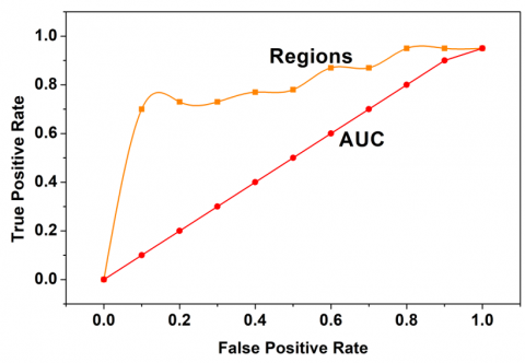
First, in Figure 7, the AUC analysis using false positives and true positives are presented. In the above Figure 7 the AVC analyses for features and regions are presented. The $\operatorname{Fext}_{\mathrm{x}}\left(\mathrm{T}_{\mathrm{i}}\right)+\operatorname{Fext}_{\mathrm{y}}\left(\mathrm{T}_{\mathrm{i}}\right)$ is jointly used for classifying x and y independently. Based on the $\operatorname{sen}_{\mathrm{v}}$ and $\operatorname{spc}_{\mathrm{f}}$ the input assessment for different $\mathrm{F}_{\mathrm{e}} \mathrm{S}^{-1}$ is observed. Through this observation, the learning intends the accuracy estimation from the contrary $\mathrm{F}_{\mathrm{e}} \mathrm{S}$ (reg. Thus the $\mathrm{B}(\mathrm{T})=\omega$ condition validates the $\mathrm{T}_{\mathrm{i}}$ for all $\Delta_{\mathrm{i}} \in \mathrm{Dfr}_{\mathrm{j}}$. The features that are not related to either of the regions are alone extracted for false positive suppression. Similarly, for the various features and regions the confusion matrix is presented in Figure 8.
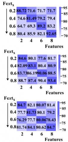
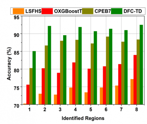
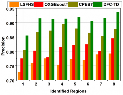
In the above Figure 8 the confusion matrix for $Fext_x$, $Fext_y$, and ${Fext }_x$+$Fext_y$ is presented. The first two represents the features for which the validation is presented. The last is the cumulative assessment for the regions identified. The $B(T)=\omega$ verification and $F_e S($reg$)$ are the valid computations for $D f r_i$ and $D f r_j$ provided $S e n_V$ and $s p c_f$ are retained. In the comparative results and discussion, the accuracy, precision, true negatives, false positives, and detection time are utilized. This analysis takes place using feature (10) and region (8) variations based on the experimental results.
Figure 8. Confusion matrix for fextx + fexty
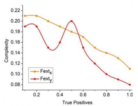
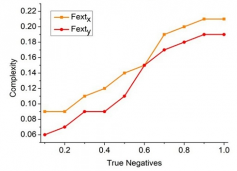
For the $\mathrm{Fext}_{\mathrm{x}}$ and $\mathrm{Fext}_{\mathrm{y}}$ discussed above, the computational complexity is analyzed in Figure 9.
The true positives leverage the region classification depending on the number of features handled. In the $F_e S$ (reg) phase, if $B(T) \neq \omega$, then true negative are identified. These true negatives are identified as the impacting factors of the $\operatorname{sen}_{\mathrm{v}}$ parameters. Therefore, the change in specificity and sensitivity (at any continuous t) requires high computations. Such computations are validated for its complexity until a new true positive is identified. This is similar for $\mathrm{Fext}_{\mathrm{x}}$ and $\mathrm{Fext}_{\mathrm{y}}$ provided to size varies (Figure 9).
The proposed method is compared with LSFHS [25], OXGBoost [21], and CPEB7 [19] methods discussed in the related works section. The methods discussed in previous studies [19, 25] are purely deep learning-based image segmentation solutions. A vision transformer process relies on the patches whereas these methods utilize the regions segmented to improve the classification. As the proposed model utilizes these two paradigms for tumor infected region detection, these methods are included as benchmark comparisons. The images where ${Fext}_x$ or ${Fext}_y$ or both are less feasible due to quality/contrast results in misclassification. Besides an image with high differentiation value results in large misclassification of true positives such that the need for new region/similar image detection is needed. Based on different features, the misclassification is reduced under various iterations.
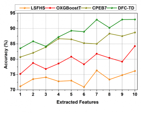
4.1 Accuracy
The proposed differential feature classification technique focuses on texture differences from the input CT images to achieve high brain tumor detection accuracy through Back-propagation learning (Refer to Figure 10). The true negatives and false positives are mitigated using extracted features from the input images to improve the feature filtering and selection. The extracted features are filtered to identify false positives and true negatives independently based on region differences in the raw image. Further, the differential feature observed in any region is represented as false positives; the identification of region-specific features from the input images using Back-propagation learning is to improve tumor detection. Hence, the features satisfying differential region identification are detected from which precise tumor region is identified in CT images. In this brain tumor detection, TN and FP observed from the current image are compared with the previous dataset for differential similarity analysis. This analysis output is to detect precise tumor regions.
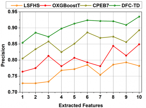
This paper achieves high brain tumor detection precision due to texture differences at the time of processing CT images at different intervals (Refer to Figure 11). The Back-propagation training process includes classified true negatives and false positives for satisfying differential region detection.
4.2 Precision
The selected features are recurrently trained to improve the feature filtering process during the extraction from distinct regions for early identification of brain tumors from the CT inputs. The differential features or true negatives in features are identified through a learning process for which region detection accuracy is improved. Both false positives and true negatives are mitigated using the conditions $F e x t \leq F e S(r e g)$ for precisely identifying the differential features through Back-propagation learning. In these extracted features filtering process, the textures may vary based on the brain tumor size observed from the CT images. The difference similarity is computed from the input images through Back-propagation learning with the accumulated textural features for identifying specific region features. In the proposed classification method, the feature selection is performed to achieve high brain tumor detection precision.
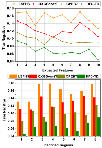
4.3 True negatives
The proposed DFC for TD achieves fewer true negatives for precise feature extraction and selection are used to find the possibilities for early brain tumor detection from the input CT image using Back-propagation learning (Refer to Figure 12). The initial training image is difficult to process until the first feature filtering is performed; this performance output is used to identify false positives and thereby reducing detection time and computation complexity. In the proposed DFC method, the extracted feature from texture differences is improved with feature classification and selection of the raw images, and hence, the precise region is detected. From the sequential feature extraction, the variations in accumulated textural features are identified for reducing true negatives. For instance, the sensitivity and specificity in employing the feature extraction are verified using Back-propagation learning to prevent true negatives. This precise feature extraction and selection is imposed to reduce the redundant features in CT images during processing. In this proposed method, the feature classification based on x and y planes at random intervals ($\varnothing \times t$) is validated for reducing true negatives and false positives.
Figure 12. True negatives
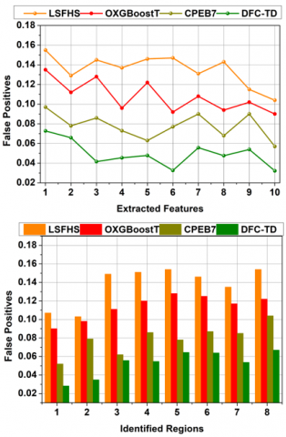
4.4 False Positives
In this proposed method, the differential features in CT images are identified to improve the precision of feature selection depending on which tumor region variations are identified with high accuracy through learning to reduce false positives (Refer to Figure 13). The redundant and unwanted features in input CT images are reduced based on the extracted feature filtering process. This process is performed to identify false positives and true negatives for region differences. Precise extracted feature filtering is processed to reduce the chances of feature variations occurring in $Input_{\partial}$. The differential feature is detected in any instance due to the redundant/unwanted features detected in the CT image at any time interval $T_{i}$. In this manner, the increasing detection time leads to fewer false positives and true negatives for inexact region detection.
Figure 13. False positives
4.5 Detection time
This proposed method is aided for maximizing feature extraction and selection from the CT images using feature filtering and Back-propagation learning for precise identification of region variations. The current data is compared with the previous dataset to satisfy less detection time as represented in Figure 14.
Figure 14. Detection time
The training process contains independent classification of true negatives and false positives are required to improve the precise feature selection for accurate region detection with less time delay and complex computations. Therefore, the direct matrix and covariance matrix function for high and low feature differences detected in a particular region is required for region-specific feature identification. Based on the difference similarity verification, the direct/ covariance matrices are used to accurately identify which tumor region contains differential features. This process is performed based on matching raw image data and malignant image data with previous datasets for accurate tumor region detection. The sensitivity and specificity of the textural features are observed and analyzed to reduce the detection time. Thus the proposed method of process feature filtering and Back-propagation learning based on region differences is to improve region detection accuracy with less detection time compared to the other factors. The comparative results and discussion tables are presented in Table 1 and Table 2.
Table 1. Comparative results and discussion for extracted features
|
Metrics |
LSFHS |
OXGBoostT |
CPEB7 |
DFC-TD |
|
Accuracy (%) |
76.16 |
84.26 |
88.72 |
92.965 |
|
Precision |
0.782 |
0.849 |
0.893 |
0.9351 |
|
True Negatives |
0.127 |
0.106 |
0.089 |
0.0449 |
|
False Positives |
0.104 |
0.09 |
0.057 |
0.0322 |
|
Detection Time (s) |
3.47 |
2.24 |
1.49 |
0.745 |
From the above Table 1, it is seen that the proposed DFC-TD improves accuracy and precision by 9.92% and 9.38%, respectively. The true negatives, false positives, and detection time are reduced by 12.49%, 10.29%, and 11.49%, respectively.
Table 2. Comparative results and discussion for identified regions
|
Metrics |
LSFHS |
OXGBoostT |
CPEB7 |
DFC-TD |
|
Accuracy (%) |
77.15 |
83.96 |
88.32 |
92.474 |
|
Precision |
0.792 |
0.845 |
0.878 |
0.9367 |
|
True Negatives |
0.178 |
0.142 |
0.123 |
0.0893 |
|
False Positives |
0.154 |
0.122 |
0.104 |
0.0669 |
|
Detection Time (s) |
3.48 |
2.41 |
1.42 |
0.977 |
From the above Table 2, it is seen that the proposed DFC-TD improves accuracy and precision by 9.33% and 9.84%, respectively. The true negatives, false positives, and detection time are reduced by 11.67%, 11.95%, and 9.97%, respectively.
From the above, it is seen that the proposed DFC-TD improves accuracy and precision by 9.33% and 9.84%, respectively. The true negatives, false positives, and detection time are reduced by 11.67%, 11.95%, and 9.97%, respectively.
In this article, the differential feature classification method for tumor detection is proposed to improve the accuracy of infected region detection. This method takes CT images as input to test, train, and validate region detection. The proposed method inherits the advantages of backpropagation learning to classify false positives and true negatives of different regions that result in false detections. The features classified are used to train the learning network that filters the high and low-impacting features promptly. Though a slight variation in the detection process is experienced, the differential region based on similar and varying features is precisely classified to improve the precision iteratively. From the experimental analysis, for the extracted features, it is seen that the proposed DFC-TD improves accuracy and precision by 9.92% and 9.38%, respectively. The true negatives, false positives, and detection time are reduced by 12.49%, 10.29%, and 11.49%, respectively.
This proposed method experiences a lag in feature differentiation during false positive extraction. This is due to the hidden feature variations in a grayscale image. The problem is generic in different CT inputs and hence, this requires a gradient equalization to reduce the classification complexity. Therefore, in the proposed work, the aforementioned issue is planned to be reduced using the equalization method.
[1] Fayaz, M., Haider, J., Qureshi, M.B., Qureshi, M.S., Habib, S., Gwak, J. (2021). An effective classification methodology for brain MRI classification based on statistical features, DWT and blended ANN. IEEE Access, 9: 159146-159159. https://doi.org/10.1109/ACCESS.2021.3132159
[2] Sekhar, A., Biswas, S., Hazra, R., Sunaniya, A.K., Mukherjee, A., Yang, L. (2021). Brain tumor classification using fine-tuned GoogLeNet features and machine learning algorithms: IoMT enabled CAD system. IEEE Journal of Biomedical and Health Informatics, 26(3): 983-991. https://doi.org/10.1109/JBHI.2021.3100758
[3] Başaran, E. (2022). A new brain tumor diagnostic model: Selection of textural feature extraction algorithms and convolution neural network features with optimization algorithms. Computers in Biology and Medicine, 148: 105857. https://doi.org/10.1016/j.compbiomed.2022.105857
[4] Shyamala, B., Brahmananda, S.D. (2023). Brain tumor classification using optimized and relief-based feature reduction and regression neural network. Biomedical Signal Processing and Control, 86: 105279. https://doi.org/10.1016/j.bspc.2023.105279
[5] Tahosin, M.S., Sheakh, M.A., Islam, T., Lima, R.J., Begum, M. (2023). Optimizing brain tumor classification through feature selection and hyperparameter tuning in machine learning models. Informatics in Medicine Unlocked, 43: 101414. https://doi.org/10.1016/j.imu.2023.101414
[6] Ramtekkar, P.K., Pandey, A., Pawar, M.K. (2023). Accurate detection of brain tumor using optimized feature selection based on deep learning techniques. Multimedia Tools and Applications, 82(29): 44623-44653. https://doi.org/10.1007/s11042-023-15239-7
[7] Bhatele, K.R., Bhadauria, S.S. (2023). Multiclass classification of central nervous system brain tumor types based on proposed hybrid texture feature extraction methods and ensemble learning. Multimedia Tools and Applications, 82(3): 3831-3858. https://doi.org/10.1007/s11042-022-13439-1
[8] Sharma, A.K., Nandal, A., Dhaka, A., Polat, K., Alwadie, R., Alenezi, F., Alhudhaif, A. (2023). HOG transformation based feature extraction framework in modified Resnet50 model for brain tumor detection. Biomedical Signal Processing and Control, 84: 104737. https://doi.org/10.1016/j.bspc.2023.104737
[9] Cheng, D., Gao, X., Mao, Y., Xiao, B., You, P., Gai, J., Mao, N. (2023). Brain tumor feature extraction and edge enhancement algorithm based on U-Net network. Heliyon, 9(11): e22536.
[10] Kumar, R.S., Nagaraj, B., Manimegalai, P., Ajay, P. (2022). Dual feature extraction based convolutional neural network classifier for magnetic resonance imaging tumor detection using U-Net and three-dimensional convolutional neural network. Computers and Electrical Engineering, 101: 108010. https://doi.org/10.1016/j.compeleceng.2022.108010
[11] Bansal, T., Jindal, N. (2022). An improved hybrid classification of brain tumor MRI images based on conglomeration feature extraction techniques. Neural Computing and Applications, 34(11): 9069-9086. https://doi.org/10.1007/s00521-022-06929-8
[12] Kumar, G.A., Sridevi, P.V. (2021). E-fuzzy feature fusion and thresholding for morphology segmentation of brain MRI modalities. Multimedia Tools and Applications, 80(13): 19715-19735. https://doi.org/10.1007/s11042-020-08760-6
[13] Woźniak, M., Siłka, J., Wieczorek, M. (2023). Deep neural network correlation learning mechanism for CT brain tumor detection. Neural Computing and Applications, 35(20): 14611-14626. https://doi.org/10.1007/s00521-021-05841-x
[14] Zhang, J., Jin, J., Ai, Y., Zhu, K., Xiao, C., Xie, C., Jin, X. (2021). Differentiating the pathological subtypes of primary lung cancer for patients with brain metastases based on radiomics features from brain CT images. European Radiology, 31: 1022-1028. https://doi.org/10.1007/s00330-020-07183-z
[15] Mohamed, D.M., Kamel, H.A. (2021). Diagnostic efficiency of PET/CT in patients with cancer of unknown primary with brain metastasis as initial manifestation and its impact on overall survival. Egyptian Journal of Radiology and Nuclear Medicine, 52: 1-8. https://doi.org/10.1186/s43055-021-00436-x
[16] Kato, S., Amemiya, S., Takao, H., Yamashita, H., Sakamoto, N., Abe, O. (2021). Automated detection of brain metastases on non-enhanced CT using single-shot detectors. Neuroradiology, 63(12): 1995-2004. https://doi.org/10.1007/s00234-021-02743-6
[17] Yu, W., Kang, H., Sun, G., Liang, S., Li, J. (2022). Bio-inspired feature selection in brain disease detection via an improved sparrow search algorithm. IEEE Transactions on Instrumentation and Measurement, 72: 1-15. https://doi.org/10.1109/TIM.2022.3228003
[18] Jabbar, A., Naseem, S., Mahmood, T., Saba, T., Alamri, F.S., Rehman, A. (2023). Brain tumor detection and multi-grade segmentation through hybrid caps-VGGNet model. IEEE Access, 11: 72518-72536. https://doi.org/10.1109/ACCESS.2023.3289224
[19] Khushi, H.M.T., Masood, T., Jaffar, A., Rashid, M., Akram, S. (2023). Improved multiclass brain tumor detection via customized pretrained EfficientNetB7 model. IEEE Access, 11: 117210-117230. https://doi.org/10.1109/ACCESS.2023.3325883
[20] Jakhar, S.P., Nandal, A., Dhaka, A., Alhudhaif, A., Polat, K. (2024). Brain tumor detection with multi-scale fractal feature network and fractal residual learning. Applied Soft Computing, 153: 111284. https://doi.org/10.1016/j.asoc.2024.111284
[21] Tseng, C.J., Tang, C. (2023). An optimized XGBoost technique for accurate brain tumor detection using feature selection and image segmentation. Healthcare Analytics, 4: 100217. https://doi.org/10.1016/j.health.2023.100217
[22] Sun, Y., Wang, C. (2024). Brain tumor detection based on a novel and high-quality prediction of the tumor pixel distributions. Computers in Biology and Medicine, 172: 108196. https://doi.org/10.1016/j.compbiomed.2024.108196
[23] Deepa, G., Mary, G.L.R., Karthikeyan, A., Rajalakshmi, P., Hemavathi, K., Dharanisri, M. (2022). Detection of brain tumor using modified particle swarm optimization (MPSO) segmentation via haralick features extraction and subsequent classification by KNN algorithm. Materials Today: Proceedings, 56: 1820-1826. https://doi.org/10.1016/j.matpr.2021.10.475
[24] Kumar, T.S., Arun, C., Ezhumalai, P. (2022). An approach for brain tumor detection using optimal feature selection and optimized deep belief network. Biomedical Signal Processing and Control, 73: 103440. https://doi.org/10.1016/j.bspc.2021.103440
[25] Kurian, S.M., Juliet, S. (2023). An automatic and intelligent brain tumor detection using Lee sigma filtered histogram segmentation model. Soft Computing, 27(18): 13305-13319. https://doi.org/10.1007/s00500-022-07457-2
[26] Brain tumor MRI and CT scan. https://www.kaggle.com/datasets/chenghanpu/brain-tumor-mri-and-ct-scan, accessed on Oct. 26, 2023.