Tamal Kumar Kundu![]() | Dinesh Kumar Anguraj*
| Dinesh Kumar Anguraj*![]()
© 2023 IIETA. This article is published by IIETA and is licensed under the CC BY 4.0 license (http://creativecommons.org/licenses/by/4.0/).
OPEN ACCESS
Malaria is a deadly disease which can be spread by the Plasmodium parasites. The existence of malaria can be identified by professional microscopists who examine the microscopic blood smear images. But it remains a challenge owing to the unavailability of experts, poor resolution images, and insufficient diagnostic quality. Therefore, image processing and machine learning (ML) models can be employed to detection of malaria parasites using blood smear images. With this motivation, this study introduces an optimal machine learning based automated malaria parasite detection and classification (OML-AMPDC) model using blood smear images. The proposed OML-AMPDC technique primarily undergoes pre-processing in two stages namely adaptive filtering (AF) based noise removal and contrast enhancement using CLAHE technique. Besides, the feature extraction process was implemented using Local Derivative Radial Patterns (LDRP). In addition, random forest (RF) classifier is applied to allot proper class labels to the blood smear images. Finally, particle swarm optimization (PSO) algorithm was utilized for optimally choose two parameters of the RF model, named maximum number of levels in every decision tree (max_depth) and number of trees in the forest (n_estimators). The design of PSO algorithm helps for enhancing the classification performance of the RF method. A wide-ranging experimental analysis is performed using benchmark dataset and the results reported the betterment of the OML-AMPDC technique over the recent approaches.
malaria parasites, disease diagnosis, blood smear images, machine learning, classification, parameter tuning
Plasmodium, a protozoan parasite that attacks red blood cells, causes malaria (RBC). Malaria is one of the main causes of juvenile neuro-disabilities, and it kills more children in Africa, where one kid dies from it every minute [1]. Thin and thick blood smears are used in a common laboratory procedure for illness analysis that is also known as the dipstick technique for diagnosis [2]. Deep learning is employed because it excels at categorizing vast volumes of data [3]. Thin and thick blood smears, which disclose characteristics including texture, location, colour, size, and morphology of the parasites from the ill patients, are diagnostic aspects of RBC presented in blood film. They signify the conventional method of illness diagnosis to all hospitals, medical labs, and clinics since it denotes a practical method for diagnosing infectious diseases like malaria [4]. The employed method conducts deep investigation of blood smear through a microscope that provides images of patient blood to clinical laboratory technologists or doctors for detecting parasites in RBC [5].
The diagnosis of blood smear images from multiple view could play vital support to diagnose the disease with minimal cost, time, and effort. In response to decreasing the workloads of the pathologist, the blood smear slide is captured effectively by using high-resolution smartphones or digital cameras [6]. The more direct the images and high its resolution, higher is the chance for accurate analysis and better results. ML approach uses algorithm based mathematical rules and statistical assumptions for learning patterns and produces meaningful classification according to the relationship of all the variables with the consequence of disease [7]. Researchers have been paying attention to deep learning in recent years, and its applications have grown exponentially [8]. In the case of sample size (n=376) is smaller to decrease meaningful classification, and authors decided that a greater number of studies will be needed [9]. Despite this, there have been challenging surveys on the ML application in different fields of malaria investigation [10].
This study presents an optimal machine learning based automated malaria parasite detection and classification (OML-AMPDC) model using blood smear images. The proposed OML-AMPDC technique involves adaptive filtering (AF) based noise removal and contrast enhancement using CLAHE technique. Moreover, the feature extraction process was implemented using Local Derivative Radial Patterns (LDRP). Furthermore, random forest (RF) classifier is employed for the appropriate class labels to the blood smear images. At last, particle swarm optimization (PSO) algorithm was used to an optimal parameter selection of the RF model, named maximum number of levels in every decision tree (max_depth) and number of trees in the forest (n_estimators). A comprehensive simulation analysis is carried out against the benchmark dataset and the outcomes revealed the enhanced performance of OML-AMPDC technique on the recent approaches. Our proposed model gives 90.33% of accuracy, 91.55% of precision, 90.42% recall and 90.28% F-score.
Rameen et al. [11] proposed a Malaria diagnosis in blood smear images through supervised learning method. The presented methodology initiates by the pre-processing stage where images are converted and resized into grayscale. The thresholding approach can be performed to recognize blobs segmentation. For feature extraction, GoogLeNet is maneuvered, and they achieved 95.8% accuracy. Narayanan et al. [12] examined the performances of different ML and DL methods for the diagnosis of Plasmodium on cell images from digital microscopy and on the testing dataset, their suggested approach delivered an overall accuracy of 96.7%. The study presents a faster CNN framework for the classifications of cell images. An automated sensing methodology with digital in-line holographic microscopy (DIHM) integrated into ML methods was introduced to sensitively diagnose unstained malaria-infected RBC (iRBC) [13]. For recognizing the RBC features, thirteen descriptors have been removed in segmentation hologram of single RBC. Six ML methods were employed for efficiently combining the prominent characteristics and to significantly enhance the diagnosis ability of the presented technique. PCA feature extraction is utilized for fetching latent components out of a higher dimension malaria vector RNA-seq data set and evaluating its classification accuracy by utilizing KNN and DT classification approaches and in that case, accuracy was 86.7% and 83.3% [14].
Bui et al. [15] study the potential of remotely sensed information, few ML and GIS classifications, and ensemble methods in the study of the nonlinear relationships among socio-physical conditions. The accurate calculation has defined by ROC curve and pair t-test. Fuhad et al. [16] introduce a fully automatic CNN based method for the diagnoses of disease under the microscopic blood smear image. Different technologies involving data augmentation, knowledge distillation, feature extraction, Autoencoder by CNN method and categorized by KNN or SVM are implemented under three training processes called autoencoder training, general training, and distillation training to improve and optimize the inference performance and model accuracy which was near about 99.23%. Masud et al. [17] proposed a DL algorithm to detect a life-threatening disease, malaria, for mobile health care solutions of patient builds an efficient mobile technique with accuracy 97.03%. The primary goal of this study is to demonstrate how DL architectures like CNN could be beneficial in real time disease diagnoses accurately and effectively in an input image and to decrease manual labour with mobile applications.
In their study, Penas et al. employed a convolutional neural network and found that it could detect malaria parasites with an accuracy of 92.4% and sensitivity of 95.2% and distinguish the two species of Plasmodium falciparum and Plasmodium vivax with an accuracy of 87.9% [18]. Pre-processing techniques were used by Umer et al. [19] to re-sample and normalize the raw microscope images. Stacked CNN was then used after being fine-tuned using max-pooling and dropout layer. A single stage evaluation of this model's performance revealed 99.98% accuracy in the identification of malaria parasites [20]. Vijayalakshmi et al. proposed a brand-new deep neural network model which was presented for transfer learning-based identification of falciparum malaria parasite infection. By combining the current Support Vector Machine (SVM) and Visual Geometry Group (VGG) networks, the suggested transfer learning technique may be accomplished (SVM). The performance of the VGG19-SVM was examined using digital photographs of malaria, and the results showed a classification accuracy of 93.1% in identifying infected falciparum malaria [21]. For multi-stage malaria parasite identification and classification, Li et al.'s DTGCN, which comprises of a CNN-based feature extractor, a source transfer graph building component, and an unsupervised GCN, is recommended [22]. Modern one-stage and two-stage object detection algorithms will be examined by Abdulrahman et al. for automated malaria parasite screening from microscopic images of thick blood slides. Performance assessments of the suggested models are carried out at the object level using mean average precision (mAP), precision, recall, F1 score, average IOU, and inference time in frames per second (FPS) [23]. To improve the precision of malaria diagnosis, Alnussary et al. developed a deep convolutional neural network (CNN) using patches segmented from microscopic pictures of red blood cell smears. Three CNN pre-trained models, including VGG19, ResNet50, and MobileNetV2, are used to create the automated parasite identification in blood from Giemsa-stained smears. They suggested accuracy of close to 100 percent [24]. To identify and categories malaria, Razin et al. presented an architecture combining the YOLOv5 algorithm with Convolutional Neural Network (CNN) [25].
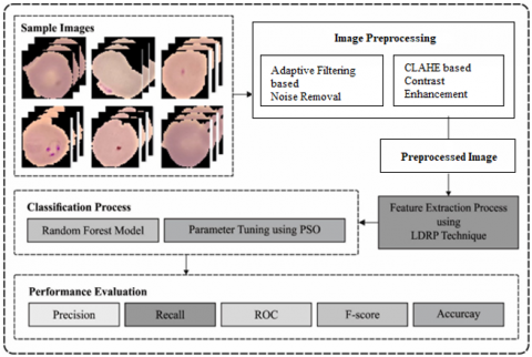
To our knowledge, we could not find comparable literature that perform CLAHE based contrast enhancement with LDRP based feature extracting technique with right class labels for the blood smear image are assigned using the Random Forest (RF) classifier. When choosing the best parameters for the RF model, the particle swarm optimization (PSO) approach was finally chosen. In this study, the OML-AMPDC technique has been presented to detection and classification of malaria parasites using blood smear images. Figure 1 demonstrates the overall block diagram of proposed OML-AMPDC technique.
Figure 1. Overall block diagram of OML-AMPDC technique
3.1 Image pre-processing
Primarily, image pre-processing is carried out in two levels namely AF based removal of noise existing in the blood smear image, and CLAHE technique was utilized for improving the contrast level of the images.
3.1.1 Adaptive filtering-based noise removal
Generally Adaptive filter has been utilized in an expansive scope of use for few decades. It is a digital linear filter with an auto-adjusting characteristics which comprises of transfer function by variable parameters and a way to change those parameters as per an optimization algorithm. It adjusts consequently to changes in its input signals. The defilement of a sign of interest by other undesirable signal or noise is an issue frequently experienced in numerous applications. Where the signal and noise possess fixed and separate frequency bands, regular linear filters with fixed coefficients are ordinarily used to extricate the signals.
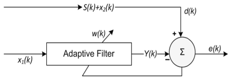
Figure 2. Schematic of adaptive filter
In Figure 2 D(k) represents desired signal, X(k) represents observation, Y(k) represents estimated D(k) and E(k) is used to represents error signal.
In any case, there are many occasions when it is fundamental for the filter attributes to be variable, adjusted to changing signal qualities or to be modified astutely. In such cases, the coefficients of the filter should change and can't be determined ahead of time. Such is the situation where there is a phantom cross-over between the signal and noise or on the other hand if the band involved by the noise is obscure or differs with time. Adaptive filters are utilized in the accompanying cases:
At the point when it is vital for the filter qualities to be variable, adjusted to changing circumstances.
At the point when there is spectral cross-over among signal and noise.
On the off chance that the band involved by the noise is obscure or variables with time.
The utilization of traditional filters in the above cases would lead to unsuitable bending of the ideal signal. An unknown system mainly recognized by this filter which a common use AF like plotting of the frequency response of an unknown communication channel. Additionally, channel recognition and echo cancellation are major notable uses of this filter. The estimated error calculation is defined in
$e(k)=d(k)-y(k)$
where, e(k) is estimated error.
The unknown system and the AF both are parallel in Figure 3.
Figure 3. System identification using adaptive filter
which is used for unknown system recognition. The square box part is represented here as an adaptive filter system. From that the e(k) values decreases that’s why the filter response is closer to the unknown system. For system recognition need three parameters first one is LMS algorithm, second one is alien / unknown system and the third one is required data set for adoption process. In Figure 4, In setting of the overall LMS model, according to d(k) & x(k) are the expected and input signal.
Figure 4. Noise canceller using adaptive filter
In this study, AF was utilized as noise canceller. In this analysis, the acoustic input signal has utilized, and noise created by microphone was lesser and create that AF makes substantial outcomes [18]. The attained error amongst output as well as predictable output signal was provided in Eq. (1).
$e(k)=\left[s(k)+x_2(k)\right]-y(k)$ (1)
Vimal et al. [26] discuss different adaptive filtering schemes with comparisons between them in their paper.
3.1.2 CHAHE based contrast enhancement
CLAHE is a type of Adaptive Histogram Equalization (AHE) approach. The majority of contrast enhancement techniques are based on global or local histogram modifications. By performing local contrast enhancement, the Contrast Limited Adaptive Histogram Equalization (CLAHE) method can circumvent the limitations of global approaches which is discussed by Campos et al. [27].
CLAHE resolves the amplification problems of traditional AHE by utilizing the several tiles parameter and clip limit. CLAHE splits the images into MxN local tiles. For all the tiles, histogram is individually computed. For computer histogram, evaluate standard amount of pixel for each region as follows
$\mathrm{N}_{\mathrm{A}}=\left(\mathrm{N}_{\mathrm{X}} \times \mathrm{N}_{\mathrm{Y}}\right) / \mathrm{N}_{\mathrm{G}}$ (2)
where, NA represent the standard number of pixels, NX indicates the amount of pixels from the X dimensional and NY indicates the amount of pixels under the Y dimensional and NG signifies the amount of gray levels. Next, determine the clip limit as follows
$\mathrm{N}_{\mathrm{CL}}=\mathrm{N}_{\mathrm{A}} \times \mathrm{N}_{\mathrm{NCL}}$ (3)
Here, NCL indicates the clip limits and NNCL denotes the standardized clip limit among zero and one Next, for all the tiles, the clip limit was employed to the height of histogram as follows.
$H_i=\left\{\begin{array}{cc}N_{C L} & \text { if } N_i \geq N_{C L} \\ N_i & \text { else }\end{array} \quad i=1,2, \ldots, 1-1\right.$ (4)
in which, Hi signifies the height of histogram of ith tile, Ni means the histogram of ith tile and L implies the amount of gray levels [19]. The overall amount of clipped pixels is evaluated by the following equation
$\mathrm{N}_{\mathrm{c}}=\left(\mathrm{N}_{\mathrm{X}} \times \mathrm{N}_{\mathrm{Y}}\right)-\sum_{\mathrm{i}=0}^{\mathrm{L}-1} \mathrm{H}_{\mathrm{i}}$ (5)
While Nc indicates 4r5 the amount of clipped pixels. Afterward evaluating Nc, redistribute the clipped pixels. The pixel is redistributed non‐uniformly or uniformly. In order to calculate the amount of pixels to be rearranged utilize the following equation
$N_R=N_C / L$ (6)
where, NR denotes the amount of pixels that redistributed. Next, the clipped histogram is standardized by the following equation
$H_i=\left\{\begin{array}{cc}N_{C L} & \text { if } N_i+N_R \geq N_{C L} \\ N_i+N_R & \text { else }\end{array} \,\, i=1,2, \ldots, l-1\right.$ (7)
The amount of undistributed pixels is calculated by Eq. (5) and (6). Till each pixel is redistributed, Eq. (7) is iterated. Eventually, cumulative histogram of the contextual regions is formulated as follows
$C_i=\frac{1}{\left(N_X \times N_Y\right)} \sum_{j=0}^i H_j$ (8)
Afterward, the calculation is accomplished, the histogram of contextual regions is equivalent with exponential or Rayleigh probability, uniform distribution, that offers a prefixed visual quality and brightness. Note that, pixel P(x,y) with value of s and 4 center point belongs to neighboring tiles that are named R1, R2, R3, and R4. The weighted sum is calculated through this contextual region. For the output image, tile is combined and eliminate the artefacts among the independent tiles were made by utilizing the bi-linear interpolation, the novel value of s has represented as follows.
$s^{\prime}=(1-y)\left((1-x) \times R_1(s)+x \times R_2(s)\right) +y\left((1-x) \times R_3(s)+x \times R_4(s)\right)$ (9)
Afterward this step, the enhanced images are attained.
3.2 LDRP based feature extraction
During feature extraction stage, the pre-processed blood smear images are passed as input to the LDRP model for the generation of feature vectors. As described, LTP and LBP is considered as general definition of micropattern that is able to define the texture without extracting a greater amount of data from the relationships among neighboring pixels. At the same time, LDP was acquired from LBP in various directions and high‐order derivatives. The LVP has presented for the redundancy reduction and accuracy improvement of earlier studies that extract various 2D spatial structures of the images with utilize of CST approach. The abovementioned pattern is depending on gray‐level difference among its Neighbors and the referenced pixel along with integration of binary coding of this difference. Due to binary coding in this pattern, a greater number of image data is lost. Mostly, the abovementioned methodologies could not define the radial pattern. Therefore, we presented LDRP that, different from the aforementioned pattern, employs radial pattern and multilevel coding rather than binary coding and rotational patterns, correspondingly.
Now, present a group of features according to the initial‐order derivative of images. To determine this feature, four directions 0°, 45°, 90°, and 135° are considered [28]. The position of the nth pixel relation to gc in α direction is represented as gα,n. gc is the reference pixel as:
$g_c=g_{0^{\circ}, 1}=g_{45^{\circ}, 1}=g_{90^{\circ}, 1}=g_{135^{\circ}, 1}$ (10)
For the I image with k gray‐level, when I(gc) represents the gray‐levels of pixel gc, the initial‐order derivatives of gc with α direction is determined by:
$I_\alpha^1\left(g_c\right)=I_\alpha^1\left(g_{\alpha, 1}\right)=I\left(g_{\alpha, 2}\right)-I\left(g_{\alpha, 1}\right)$ (11)
Consider the abovementioned equations for all the images, the four matrices are extracted by: $I_{0 \circ}^1, I_{45^{\circ}}^1, I_{90^{\circ}}^1$ and $I_{135^{\circ}}^1$. As the images have k gray‐level, 2 neighboring pixels takes value from 0 to k-1 which results in distinct values for $I_\alpha^1$ and hence, $I_\alpha^1$ might take 2k-1 integer values:
$I_\alpha^1 \in Z,-(k-1) \leq I_\alpha^1 \leq(k-1)$ (12)
Here, we determine a sequence of features according to the derivative which could determine local pattern. Hence, select them as LDRP and they are signified as $L D R P_{P, \alpha}^n$. In this description, P, and α represents order of derivative, amount of neighboring pixels under the pattern, and design direction, correspondingly.
3.3 RF based classification
At the time of classification process, the RF model is utilized to allot proper class of the input blood smear images. The RF is an ensemble classification which has several DTs. It can be a group of tree predictor effects that all trees based on values of arbitrary vector sampled individually and with similar distribution to every tree under the forest. Once a novel record acts like input, RF puts it down to all trees under the forest. All trees provide a classifier, and the forest select that class is ordered by most of the trees [29].
The RF algorithm works as follows:
Select T amount of trees for growing.
Select m amount of variables utilized for splitting all nodes. m<<M, where M refers the amount of input variables.
Grow trees, but growing all trees, do the subsequent:
Create the instance of size N in N trained cases with replacement and growing a tree in this novel instance.
Once the developing a tree at all nodes, choose m variables at arbitrary in M and utilize them for finding optimum splits.
Develop the tree to higher extents. There is no pruning.
For classifying point X, gather the vote in all trees under the forest also utilize popular voting for deciding on class label.
|
Algorithm 1: Random Forest for Classification |
|
for n=1;k≤K;k=k+1 do Derive the bootstrap instance Z of size M under the trained data. Develop the RF tree Tk to bootstrapped data, with recursively repeated the subsequent steps to all end nodes of tree, still the minimal node size mmin has attained. i. Choose m variables at arbitrary in the p variables. ii. Select the optimum variable/ separate-point amongst the m; iii. Separate the node as to 2 leaf nodes. Result in the ensemble of trees $\left\{T_k\right\}_1^K$; For making the forecast at novel point x: Assume that fk(x) be the class forecast of bth RF tree. Next $f_{R F}(x)= majority \,\,vote \left\{f_k(x)\right\}_1^K$. |
3.4 PSO based parameter tuning
For optimally adjusting the parameters of the RF model (max_depth and n_estimators), the PSO algorithm is utilized and thereby boosting the detection efficiency. The PSO is a technique dependent upon SI that is initially presented by Kenndy and Eberhart in 1995 [30]. Due to their simplicity from execution, the PSO technique was effectively utilized from ML, adaptive control, signal processing, etc. In the initial phase, the population of m particles is established arbitrarily, all particles are a potential solution to challenge that requires for resolved from the search space. During all iterations, the velocity as well as place of all the particles were upgraded utilizing 2 values: one is the optimum value (pb) of particle, and another is optimum value (gb) of population entire previous. Let us m particle from the d dimension search space, the velocities as well as places of l^th particle at time of z is written as:
$\begin{aligned} & v_l(z)=\left[v_{l 1}(z), v_{l 2}(z), \cdots, v_{l d}(z)\right]^z \\ & x_l(z)=\left[x_{l 1}(z), x_{l 2}(z), \cdots, x_{l d}(z)\right]^z\end{aligned}$
An optimum value of particle and the entire previous optimum value of population at round t are.
$\begin{aligned} p_{b l}(z) & =\left[p_{l 1}(z), p_{l 2}(z), \cdots, p_{l d}(z)\right]^Z \\ g_b(z) & =\left[g_1(z), g_2(z), \cdots, g_d(z)\right]^Z\end{aligned}$
At iteration z+1, the place as well as velocity of particle were upgraded as:
$v_l(z+1)=\omega v_l(z)+c_1 r_1\left(p_{b l}(z)-x_l(z)\right)+c_2 r_2\left(g_b(z)-x_l(z)\right)$ (13)
$x_l(z+1)=x_l(z)+v_l(z+1)$ (14)
where, ω refers the inertia weight coefficients that are trade-off global search capability against local search capability; c1 and c2 are learning factors of technique. When c1=0, it can be simple to fall as to local optimized and could not jump out; once c2=0 it would generate illustrate convergence speed of PSO; r1 and r2 represents the arbitrary variables uniformly distributed from zero and one. Figure 5 illustrates the flowchart of PSO technique.
During all iterations of PSO technique [31], only the optimum particle is transferred from the data to another particle. This technique usually is 2 end criteria’s: a maximal amount of iterations or appropriately optimum fitness value.
The procedure of PSO is as follows.
The PSO method derivative a FF for attaining enhanced classification performance. It defines as positive integer for representing the optimum efficiency of candidate solutions. During this analysis, the minimized classifier error rate was There are three Figure 5 in the manuscript, which clearly does not meet the requirements of the journal. Regarded FF, as provided in Eq. (15). The optimum solution is lesser error rate and least solution gains a higher error rate.
${ fitness }\left(x_i\right)={ ClassifierErrorRate }\left(x_i\right) = \frac{{ numerb\,\, of\,\, misclassified\,\, images }}{{ Total\,\, number\,\, of\,\, images }} \quad* 100$ (15)
Figure 5. Flowchart of PSO method
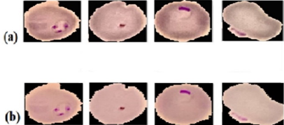
The experimental result analysis of the proposed technique takes place on the benchmark Malaria dataset [32]. The dataset includes 27558 images including 13779 parasitized images and 13779 uninfected images. Besides, the dataset is split as to training/testing data with a ratio of 70:30. The proposed model is simulated using Python 3.6.5 tool. The sample visualization result analysis of the OML-AMPDC technique is offered in Figure 6.
Figure 6. Sample Images (a) Parasitized (b) Uninfected
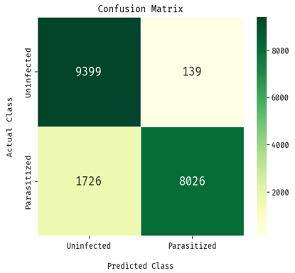
The first row depicts the original blood smear image, and the respective pre-processed image is depicted in Figure 7. Besides, it is evident that the quality of the blood smear image gets considerably improved. Below in Figure 8 demonstrates the confusion matrix generated by the OML-AMPDC technique on the training dataset. The figure revealed that the OML-AMPDC technique has classified 9399 images into Uninfected class and 8026 images into Parasitized images.
Figure 7. Sample results (a) Original Images (b) Pre-processed Images
Figure 8. Confusion matrix of OML-AMPDC approach on training dataset
Figure 9. ROC analysis of OML-AMPDC technique on training dataset
In the above Figure 9 exhibits the ROC analysis of the OML-AMPDC technique on the test training data which shown in below. The figure revealed that the OML-AMPDC technique has accomplished maximum ROC of 0.90.
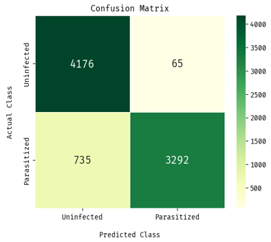
Similarly in the Figure 10 portrays the confusion matrix generated by the OML-AMPDC method on the testing dataset. The figure depicted that the OML-AMPDC algorithm has classified 4176 images into Uninfected class and 3292 images into Parasitized images.
Figure 10. Confusion matrix of OML-AMPDC technique on testing dataset
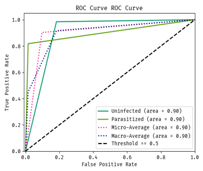
In the Figure 11 defines the ROC analysis of the OML-AMPDC algorithm on the test testing data. The figure exposed that the OML-AMPDC method has accomplished maximal ROC of 0.90.
Figure 11. ROC analysis of OML-AMPDC approach on testing dataset
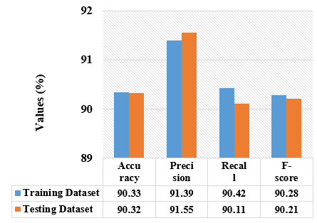
Table 1 and Figure 12 offer a brief result analysis of the OML-AMPDC technique on the test training and testing dataset.
On the applied training dataset, the OML-AMPDC technique has resulted in accuracy of 90.33%, precision of 91.39%, recall of 90.42%, and F-score of 90.28%. Similarly, on the applied testing dataset, the OML-AMPDC algorithm has resulted in accuracy of 90.32%, precision of 91.55%, recall of 90.11%, and F-score of 90.21%.
Table 1. Result analysis of OML-AMPDC Method with training and testing dataset
|
Measures |
Training Dataset |
Testing Dataset |
|
Accuracy |
90.33 |
90.32 |
|
Precision |
91.39 |
91.55 |
|
Recall |
90.42 |
90.11 |
|
F-score |
90.28 |
90.21 |
Figure 12. Result analysis of OML-AMPDC technique with different measures
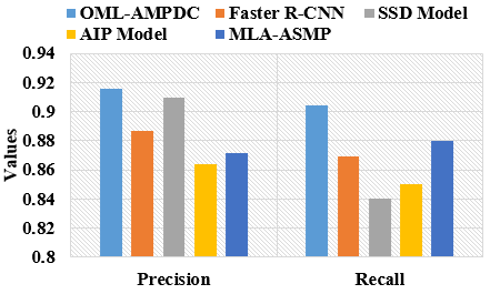
Overall comparative result analysis of the OML-AMPDC with recent methods is carried out in Table 2 [25-27]. Figure 13 illustrates the precision and recall analysis of the OML-AMPDC with existing techniques.
The results show that the Faster RCNN, MLA-ASMP, and AIP techniques have obtained least performance with the minimal values of precision and recall. Next, the SSD approach has showcased slightly enhanced outcomes with the precision and recall of 0.9100 and 0.8400. However, the OML-AMPDC technique has outperformed the other methods with the precision and recall of 0.9155 and 0.9042.
Table 2. Comparative analysis of OML-AMPDC technique with existing approaches
|
Methods |
Precision |
Recall |
Accuracy |
F-score |
|
OML-AMPDC (Proposed model) |
0.9155 |
0.9042 |
0.9033 |
0.9028 |
|
Faster R-CNN |
0.8865 |
0.8690 |
0.8980 |
0.8971 |
|
SSD Model |
0.9100 |
0.8400 |
0.8750 |
0.8700 |
|
AIP Model |
0.8643 |
0.8500 |
0.7300 |
0.8512 |
|
MLA-ASMP |
0.8712 |
0.8798 |
0.8400 |
0.8685 |
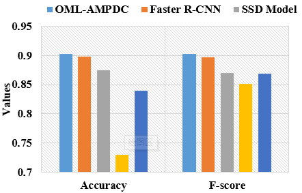
Figure 14 demonstrates the accuracy and F-measure analysis of the OML-AMPDC with recent techniques. The outcomes illustrated that the SSD, MLA-ASMP, and AIP methodologies have obtained minimum performance with lower values of accuracy and F-measure. Followed by, the Faster RCNN technique has showcased somewhat improved outcomes with accuracy and F-measure of 0.8980 and 0.8971. However, the OML-AMPDC algorithm has exhibited the other approaches with the accuracy and F-measure of 0.9033 and 0.9028.
From the detailed results and discussion, it is obvious that the OML-AMPDC technique has accomplished better performance over the other techniques. Therefore, the OML-AMPDC technique can be applied as an effective tool for malaria parasite detection.
Figure 13. Precision and recall analysis of OML-AMPDC technique
Figure 14. Accuracy and F-measure analysis of OML-AMPDC technique
In this study, the OML-AMPDC technique has been presented for the detection and classification of malaria parasites using blood smear images. The proposed OML-AMPDC technique encompasses several subprocesses namely AF based noise removal, CLAHE based contrast enhancement, LDRP based feature extraction, RF based classification, and PSO based parameter optimization. The design of the PSO algorithm fine tunes the two parameters of the RF model (max_depth and n_estimators), and thereby improves the detection accuracy. A comprehensive simulation analysis is carried out against the benchmark dataset and the outcomes revealed the enhanced performance of the OML-AMPDC technique over the recent approaches. Therefore, the OML-AMPDC technique can be utilized as an effective tool for malaria parasite diagnosis. As a part of future extension, the classification performance of the OML-AMPDC technique can be boosted by the use of image segmentation approaches.
|
D(k) |
desired signal |
|
X(k) |
observation |
|
Y(k) |
estimated D(k) and E(k) is used to represents error signal |
|
e(k) |
estimated error |
|
d(k) |
expected signal |
|
x(k) |
input signal |
|
NA |
standard amount of pixels |
|
NX |
amount of pixels from the X dimensional |
|
NY |
amount of pixels under the Y dimensional |
|
NG |
amount of gray levels |
|
NNCL |
standardized clip limit among zero and one |
|
NCL |
indicates the clip limits |
|
Hi |
height of histogram of ith tile |
|
Ni |
histogram of ith tile |
|
L |
amount of gray levels |
|
P(x,y) |
pixel |
|
NR |
amount of pixels that redistributed |
|
R1, R2, R3, R4 |
four center points |
|
gc |
reference pixel |
|
I(gc) |
gray‐levels of pixel gc |
|
gα,n |
nth pixel relation to gc in α direction |
|
$I_\alpha^1\left(g_c\right)$ |
1st order derivatives of gc with α direction |
|
$L D R P_{P, \alpha}^n$. |
P, and α represents order of derivative, amount of neighboring pixels under the pattern, and design direction, correspondingly |
|
T |
amount of trees |
|
m |
amount of variables utilized for splitting all nodes |
|
M |
amount of input variables |
|
N |
trained case |
|
X |
classifying point |
|
Z |
bootstrap instance |
|
Tk |
RF tree |
|
mmin |
minimal node size |
|
$\left\{T_k\right\}_1^K$ |
ensemble of trees |
|
fk(x) |
class forecast of bth RF tree |
|
$\left\{f_k(x)\right\}_1^K$ |
majority vote |
|
pb |
optimum value of particle |
|
gb |
optimum value of population |
|
d |
dimension search space |
|
m |
number of particle |
|
z |
bootstrap instance |
|
c1, c2 |
learning factors |
|
r1, r2 |
arbitrary variables uniformly distributed from zero and one |
|
(xi) |
fitness or classifier error rate |
|
Greek symbols |
|
|
ω |
inertia weight |
|
α |
direction |
[1] Pal, M., Brata, K., Kumar, S., Sabin, L.L. (2019). The economic cost of malaria at the household level in high and low transmission areas of central India. Acta Tropica, 190: 344-349. https://doi.org/10.1016/j.actatropica.2018.12.003
[2] Rajaraman, S., Jaeger, S., Antani, S.K. (2019). Performance evaluation of deep neural ensembles toward malaria parasite detection in thin-blood smear images. PeerJ., 7: e6977. https://doi.org/10.7717/peerj.6977
[3] Çinar, A., Yildirim, M. (2020). Classification of malaria cell images with deep learning architectures. Ingénierie des Systèmes d’Information, 25(1): 35-39. https://doi.org/10.18280/isi.250105
[4] Esayas, E., Woyessa, A., Massebo, F. (2020). Malaria infection clustered into small residential areas in lowlands of southern Ethiopia. Parasite Epidemiol Control, 10: e00149. https://doi.org/10.1016/j.parepi. 2020.e00149
[5] Hegde, R.B., Prasad, K., Hebbar, H., Sandhya, I. (2018). Peripheral blood smear analysis using image processing approach for diagnostic purposes: A review. Biocybernetics and Biomedical Engineering, 38(3): 467-480. https://doi.org/10.1016/j.bbe.2018.03.002
[6] Rajaraman, S., Antani, S.K., Poostchi, M., Silamut, K., Hossain, A., Maude, R.J., Jaeger, S., Thoma, G.R. (2018). Pre-trained convolutional neural networks as feature extractors toward improved malaria parasite detection in thin blood smear images. PeerJ, 6: e4568. https://doi.org/10.7717/peerj.4568
[7] Poostchi, M., Silamut, K., Maude, R.J., Jaeger, S., Thoma, G. (2018). Image analysis and machine learning for detecting malaria. Translational Research, 194: 36-55. https://doi.org/10.1016/j.trsl.2017.12.004
[8] Alqudah, A., Alqudah, A.M., Qazan, S. (2020). Lightweight deep learning for malaria parasite detection using cell-image of blood smear images. Revue d'Intelligence Artificielle, 34(5): 571-576. https://doi.org/10.18280/ria.340506
[9] Thakur, S., Dharavath, R. (2019). Artificial neural network-based prediction of malaria abundances using big data: A knowledge capturing approach. Clinical Epidemiology and Global Health, 7(1): 121-126. https://doi.org/10.1016/j.cegh.2018.03.001
[10] Morang’a, C.M., Amenga-Etego, L., Bah, S.Y., Appiah, V., Amuzu, D.S., Amoako, N., Abugri, J., Oduro, A.R., Cunnington, A.J., Awandare, G.A., Otto, T.D. (2020). Machine learning approaches classify clinical malaria outcomes based on haematological parameters. BMC Medicine, 18(1): 1-16. https://doi.org/10.1186/s12916-020-01823-3
[11] Rameen, I., Shahadat, A., Mehreen, M., Razzaq, S., Asghar, M.A., Khan, M.J. (2021). Leveraging supervised machine learning techniques for identification of malaria cells using blood smears. In 2021 International Conference on Digital Futures and Transformative Technologies (ICoDT2), Islamabad, Pakistan, pp. 1-6. https://doi.org/10.1109/ICoDT252288.2021.9441534
[12] Narayanan, B.N., Ali, R., Hardie, R.C. (2019). Performance analysis of machine learning and deep learning architectures for malaria detection on cell images. In Applications of Machine Learning, 11139: 111390W. https://doi.org/10.1117/12.2524681
[13] Go, T., Kim, J.H., Byeon, H., Lee, S.J. (2018). Machine learning‐based in‐line holographic sensing of unstained malaria‐infected red blood cells. Journal of Biophotonics, 11(9): e201800101. https://doi.org/10.1002/jbio.201800101
[14] Arowolo, M.O., Adebiyi, M., Adebiyi, A.A., Okesola, J.O. (2020). PCA model for RNA-Seq malaria vector data classification using KNN and decision tree algorithm. 2020 International Conference in Mathematics, Computer Engineering and Computer Science (ICMCECS), Ayobo, Nigeria. https://doi.org/10.1109/ICMCECS47690.2020.240881
[15] Bui, Q.T., Nguyen, Q.H., Pham, V.M., Pham, M.H., Tran, A.T. (2019). Understanding spatial variations of malaria in Vietnam using remotely sensed data integrated into GIS and machine learning classifiers. Geocarto International, 34(12): 1300-1314. https://doi.org/10.1080/10106049.2018.1478890
[16] Fuhad, K.M., Tuba, J.F., Sarker, M., Ali, R., Momen, S., Mohammed, N., Rahman, T. (2020). Deep learning based automatic malaria parasite detection from blood smear and its smartphone based application. Diagnostics, 10(5): 329. https://doi.org/10.3390/diagnostics10050329
[17] Masud, M., Alhumyani, H., Alshamrani, S.S., Cheikhrouhou, O., Ibrahim, S., Muhammad, G., Hossain, M.S., Shorfuzzaman, M. (2020). Leveraging deep learning techniques for malaria parasite detection using mobile application. Wireless Communications and Mobile Computing, 2020: 8895429. https://doi.org/10.1155/2020/8895429
[18] Peñas, K.E.D., Rivera, P.T., Naval, P.C. (2017). Malaria parasite detection and species identification on thin blood smears using a convolutional neural network. In 2017 IEEE/ACM International Conference on Connected Health: Applications, Systems and Engineering Technologies (CHASE), Philadelphia, PA, USA, pp. 1-6. https://doi.org/10.1109/CHASE.2017.51
[19] Umer, M., Sadiq, S., Ahmad, M., Ullah, S., Choi, G.S., Mehmood, A. (2020). A novel stacked CNN for malarial parasite detection in thin blood smear images. IEEE Access, 8: 93782-93792. https://doi.org/10.1109/ACCESS.2020.2994810
[20] Vijayalakshmi, A. (2020). Deep learning approach to detect malaria from microscopic images. Multimedia Tools and Applications, 79: 15297-15317. https://doi.org/10.1007/s11042-019-7162-y
[21] Li, S., Du, Z.Y., Meng, X.J., Zhang, Y. (2021). Multi-stage malaria parasite recognition by deep learning. GigaScience, 10(6): giab040. https://doi.org/10.1093/gigascience/giab040
[22] Abdurahman, F., Fante, K.A., Aliy, M. (2021). Malaria parasite detection in thick blood smear microscopic images using modified YOLOV3 and YOLOV4 models. BMC Bioinformatics, 22(1): 1-17. https://doi.org/10.1186/s12859-021-04036-4
[23] Chakradeo, K., Delves, M., Titarenko, S. (2021). Malaria parasite detection using deep learning methods. International Journal of Computer and Information Engineering, 15(2): 175-182. https://doi.org/10.5281/zenodo.4569849
[24] Razin, W.R.W.M., Gunawan, T.S., Kartiwi, M., Yusoff, N.M. (2022). Malaria parasite detection and classification using CNN and YOLOv5 architectures. In 2022 IEEE 8th International Conference on Smart Instrumentation, Measurement and Applications (ICSIMA), Melaka, Malaysia, pp. 277-281. https://doi.org/10.1109/ICSIMA55652.2022.9928992
[25] Alnussairi, M.H.D., İbrahim, A.A. (2022). Malaria parasite detection using deep LEARNING algorithms based on (CNNs) technique. Computers and Electrical Engineering, 103: 108316. https://doi.org/10.1016/j.compeleceng.2022.108316
[26] Vimal, V., Khosla, A., Prabhakar, P., Arora, S., Ashok, A. (2021). Comparison of adaptive filtering scheme for sustainable and efficient communication in smart city. Sustainable Energy Technologies and Assessments, 47: 101472. https://doi.org/10.1016/j.seta.2021.101472
[27] Campos, G.F.C., Mastelini, S.M., Aguiar, G.J., Mantovani, R.G., Melo, L.F.D., Barbon, S. (2019). Machine learning hyperparameter selection for contrast limited adaptive histogram equalization. EURASIP Journal on Image and Video Processing, 2019(1): 1-18. https://doi.org/10.1186/s13640-019-0445-4
[28] Fadaei, S., Amirfattahi, R., Ahmadzadeh, M.R. (2017). Local derivative radial patterns: A new texture descriptor for content-based image retrieval. Signal Processing, 137: 274-286. https://doi.org/10.1016/j.sigpro.2017.02.013 0165-1684
[29] Malik, A.J., Shahzad, W., Khan, F.A. (2015). Network intrusion detection using hybrid binary PSO and random forests algorithm. Security and Communication Networks, 8(16): 2646-2660. https://doi.org/10.1002/sec.508
[30] Bai, Q. (2010). Analysis of particle swarm optimization algorithm. Computer and Information Science, 3(1): 180. https://doi.org/10.5539/cis.v3n1p180
[31] Li, Y., Zhang, Y. (2020). Hyper-parameter estimation method with particle swarm optimization. arXiv preprint arXiv:2011.11944. https://doi.org/10.48550/arXiv.2011.11944
[32] https://lhncbc.nlm.nih.gov/LHC-publications/pubs/MalariaDatasets.html, accessed on 1 July 2021.