Recognizing Chinese Predicate Heads Based on Textual Bounding Boxes

A predicate head (or predicate in short) is a verbal expression that plays a role as the structural center of a sentence. It is the central grammatical role to organize relevant syntactic elements in a sentence, e.g., subject, object, etc. Therefore, identifying the predicate is the key to understanding a sentence. Unlike many synthetic languages, e.g., English, they have affluent inflections to express syntactic relationships between words, recognizing predict head in Chinese is difficult. There are six distinctive characteristics, which makes the task to identify Chinese predicates more challenging.

First, Chinese is an ancient hieroglyphic. Chinese characters (or Hanzi) are ideograms where every character can convey a specific concept. Chinese hosts a large number of characters. Every Chinese character can be used as a word or as a morpheme, which considerably increases the searching space for predicate recognition. Second, a Chinese sentence is a sequence of characters, where a Chinese word is consisted of one or more characters without delimitation between them. Identifying predicates suffers from serious segmentation ambiguities. Third, Chinese verbs are usually multi-categorical in terms of part-of-speech (POS), without morphology indicating their verbal usages. Fourth, the predicate head in a Chinese sentence depends on its syntactic features of words. However, because Chinese is a hieroglyphic language, it is unable to depend on form and tense of words. Fifth, Chinese verbal expressions are often dynamically generated by rules or patterns. It is impossible to hold a predefined verb dictionary. Sixth, a Chinese sentence often contains several verbs. For example, in the one month of People’s Daily corpus [1], 30% sentences are manually annotated with successive verbs. Distinguishing predicate from verbs is ambiguous, because each of these verbs can be considered as a predicate or as an adverbial phrase. Therefore, recognizing predicates in a Chinese sentence is a challenging task.

Recognizing Chinese predicates can be modeled as a sequence labeling task, where every character has predicated a tag to indicate its role in a predicate. For example, in the B-“I-O” encoding, tags of a character “B”, “I” and “O” indicates that it is a start, inside or outside of a predicate. Given a sentence as input, a sequence model (e.g., Hidden Markov Model (HMM) [2, 3], Conditional Random Field (CRF) [4], or Long Short-Term Memory (LSTM) [5]) outputs a maximized label sequence for identifying predicates. Because the predicate is defined as the structural center of a sentence, a sentence usually contains only a predicate. Therefore, recognizing predicates is heavily depending on the global information of a sentence. The HMM and CRF often assume a first-order Markov dependency. They recognize a label element mainly depends on local features, which cannot ensure the output of a predicate. The LSTM uses a cell to memory the dependency information. However, when the distance is longer, the dependency information has vanished seriously.

In this paper, we propose a textual bounding box approach to support Chinese predicate recognition. In this approach, a sentence is first mapped into an abstract representation known as feature maps. Then, textual bounding boxes are generated from feature maps. A textual bounding box is an abstract representation of a possible predicate candidate. Each box has three parameters to indicate its class tag and its positions in a sentence. Because feature maps are generated by techniques such as Bi-LSTM [6] or Transformer [7], they encode semantic dependency information about a whole sentence. In the training process, for every box, in addition to predict the classification confidence, the position offset between the box and a true predicate are learned simultaneously. Compared with related works, our model has the advantage to make full use of annotation information and share parameters in the bottom of a deep neural network, which enhance model discriminability and enables more potent nonlinear function approximators for Chinese predicate heads recognition.

Before given the architecture of our model, definitions about textural bounding boxes are discussed as follows.

3.1 Textural bounding boxes

Let $X_t=\left[x_1, x_2, \ldots x_N\right]$ be a sentence, where $x_i(1 \leq i \leq N)$ is a Chinese character. A neural network is adopted to transform $X_t$ into a hidden representation denoted as $H_t=\left[h_i, h_2, \ldots, h_N\right]$. The neural network to transform $X_t$ into $H_t$ is called a basic network, which can be truncated from a standard sentence labeling architecture for named entity recognition or POS tagging (e.g., a traditional BiLSTM architecture). In the basic network, many techniques (e.g., LSTM, Attention) can be used to capture global or dependency information of a sentence. In this paper, the hidden representation $H_t$ is referred to as feature maps. Therefore, a feature map hi is a high-order abstract representation of $x_i$. The representation can encode semantic dependency and global information by a deep neural network.

A textual bounding box $d_i$ is defined as a subsequence of $H_t$ denoted as $d_i=\left[h_s, \ldots, h_{s+l}\right](1 \leq s \leq s+l \leq N)$. A textual bounding box $d_i$ can be represented as a triple $\left\langle s_j, l_j, c_j\right\rangle$. It has three parameters representing its class type, start position and length of the bounding box. Given a bounding box $d_i$, if the corresponding input characters $\left[x_s, \ldots, x_{s+l}\right]$ is a true predicate, the box is named as a grounding truth bounding box, referred as $g_j=\left\langle s_j, l_j, c_j\right\rangle$.

Given a sentence $X_t$ and its feature maps $H_t$, let Dt represent all bounding boxes generated from $H_t$. It is represented as:

 $\mathrm{D}_t=\left\{d_i \mid d_i=\left\langle s_i, l_i, c_i\right\rangle, 1 \leq s_i \leq s_i+l_i \leq n\right\}$        (1)

Because every bounding box has parameters indicating its position in a sentence. Therefore, the ratio of intersection over union (IoU) between bounding boxes and a grounding truth box can be adopted to generate positive bounding boxes and negative bounding boxes. Let A and B represent the location ranges of two bounding boxes in a sentence. The IoU between A and B is computed as:

 $\operatorname{IoU}(A, B)=\frac{A \cap B}{A \cup B}$       (2)

All positive bounding boxes have a high overlapping ratio relative to some grounding truth bounding boxes. Therefore, positive bounding boxes contains effective semantic information for position regression. Negative bounding boxes are often far away from any truth box. They are mainly used to train a classifier for distinguishing true and false predicate instances.

Let $G_t$ represents a truth bounding box set of $X_t$. The bounding box set $D_t$ can be. 

$\mathrm{D}_t\mathrm{P}=\left\{d_t \mid d_i \in \mathrm{D}_t, \exists g_j \in G_t\left(\operatorname{IoU}\left(d_i, g_j\right) \geq \gamma\right)\right\}$

$\mathrm{D}_t\mathrm{~N}=\left\{d_i \mid d_i \in \mathrm{D}_t, \exists g_j \in G_t\left(\operatorname{IoU}\left(d_i, g_j\right)<\gamma\right)\right\}$      (3)

The $D_t P$ and $D_t N$ are referred to as the positive bounding box set and the negative bounding box set.

In most of time, $D_t P$ contains a few bounding boxes, but there is a large number of negative bounding boxes in $D_t N$. This leads to a serious data imbalance problem, which influences the performance and increase the computation complexity. Therefore, the ratio of intersection over union (IoU) between bounding boxes and a grounding truth box can be adopted to remove bounding boxes that are unlikely. This strategy is helpful for avoiding the data unbalance problem. In the training data, negative bounding boxes with lower IoU values are removed.

3.2 Training objective

Given a bounding box $d_i=\left\langle s_i, l_i, c_i\right\rangle$, the true class type $c_i$ is a one-hot representation, where $c_i$=[0,1] and $c_i$=[1,0] means that it is a false predicate instance and a true predicate respectively. The true position offset between $d_i$ relative to a grounding truth bounding box gj is normalized as following:

$\hat{s}_{i j}=\left(s_j-s_i\right) / s_j \quad \hat{l}_{i j}=\log \left(l_j / l_i\right)$          (4)

In this paper, a softmax layer and a linear layer are adopted to predict its classification confidence and to learn the position offsets relative to an adjacent grounding truth bounding box. The output of the softmax layer is denoted as $\tilde{c}=\left(\tilde{c}_0, \tilde{c}_1\right)$ in with $\tilde{c}_0$ and $\tilde{c}_1$ are the probabilities to be a negative predicate and a positive predicate. The output of position offset between $d_i$ relative to a grounding truth bounding box $g_j$ is represented as $\left(\Delta s_{i j}, \Delta l_{i j}\right)$. Therefore, the total loss includes the location loss $\left(L_{l o c}(x, s, l)\right.$ and confidence loss $\left(L_{\operatorname{con}}(x, c)\right)$. It is represented as following:

$L(x, s, l, c)=L_{l o c}(x, s, l)+\alpha L_{c o n}(x, c)$          (5)

The parameter α is used to balance the weight between $L_{l o c}$ and $L_{l o c}$.

Given a bounding box $d_i \in D_t P$ and a truth box $g_j \in G_t$, let $E_{i j}=\{0,1\}$ be a characteristic function defined as follows:

 $E_{i j}=\left\{\begin{array}{lr}1, & \gamma \leq \operatorname{argmax}_{g_i \in G_t} {IoU}\left(d_i, g_i\right) \\ 0, & \ {others}\end{array}\right.$       (6)

Given a sentence $X_t$ with its corresponding truth box set $G_t$ and positive bounding box set $D_t P$, the location loss is computed as follows:

 $L_{l o c}(x, s, l)=\sum_{g_j \in G_t} \frac{1}{N}\left(\sum_{d_i \in \mathrm{D}_t \mathrm{P}} E_{i j}\left(\left|\Delta s_{i j}-\hat{s}_{i j}\right|+\left|\Delta l_{i j}-\hat{l}_{i j}\right|\right)\right)$       (7)

In Eq. (7), N denotes to the number positive bounding boxes that match to $g_j \in G_t$. The coefficient 1/N is used normalize the weight between different truth boxes. In the learning process, minimizing the $L_{l o c}(x, c)$ is used normalize the weight between different truth boxes. In the learning process, minimizing the $L_{l o c}(x, s, l)$ can result in every $d_i$ approaching to the nearest truth box $g_j$.

The confidence loss ${Lcon}(x, \ c)$ is a cross-entropy loss that is formalized as following:

$\operatorname{Lcon}(x, c)=-\sum_{d_i \in \mathrm{D}_{\mathrm{P}} \mathrm{P}} E_{i j} \log \left(\tilde{c}_1\right)-\sum_{d_i \in \mathrm{D}_{\mathrm{t}} \mathrm{N}} \log \left(\tilde{c}_0\right)$     (8)

The training objective is to reduce the total loss of the location offset and class prediction. In the training process, we optimize their locations to improve their matching degree and maximize their confidences.

3.3 Architecture of model

1.png

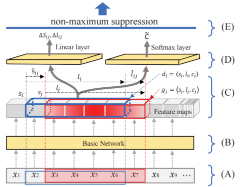
Figure 1. Architecture of model: (A) input layer,

(B) basic network, (C) bounding box generation,

(D) output layer, (E) non-maximum suppression

In this paper, we design an end-to-end multi-objective learning framework to simultaneously locate predict and the class probability. The architecture of this model is shown in Figure 1.

The architecture of the neural network is divided into five parts. Each part is discussed as follows.

(A) The input of this model is a sentence. In order to guarantee the same length for every sentence in the feature map layer, the length of sentence is set as 100. Longer sentences and shorter sentences are trimmed or padded respectively.

(B) A basic network is adopted to transform the input into feature maps. The basic network can be truncated from a standard sentence labelling architecture. In this paper, it is composed of an embedding layer and a Bi-LSTM layer. In the embedding layer, every input xi is embedded into a distributed representation. The embedding can encode dense semantic information of words by pretrained lookup table. In this model, the BERT [24] approach is adopted to support the word embedding, which transforms every word into a 768 dimensional vector. The BiLSTM is a recurrent network that consists of two LSTMs [6]. It takes the input in a forward direction and a backward direction. In each direction, a cell is used to memory the previous hidden states. Therefore, the BiLSTM is effective to learn the semantic dependency in a sentence.

(C) Outputs of the basic network are named as feature maps. They are abstract representations of a sentence. Because the recurrent work is adopted to implement feature mapping, a feature map encodes semantic information of a word and its context. Let $\left[h_1, h_2, \ldots h_N\right]$ denotes to the feature maps. According to Eq. (1), every feature map $h_i$ is assembled with right feature maps for generating a default bounding box set $\left\{\left[h_i, h_{i+1}, \ldots, h_{i+k}\right] \mid 1 \leq k \leq K\right\}$. In our experiment, 6 is set as the default value of  . Except the rightmost feature maps, it generates 6 default bounding boxes for each feature map. For each input sentence, there are 285 default bounding boxes in total. It generates a large number of negative bounding boxes, which leads to a serious imbalance problem. Eq. (3) can be used to filter bounding boxes. To reduce the computation complexity, the number of elements in $D_t P$ and $D_t N$ is limited to 1:3. 

(D) A bounding box is an abstract representation of a possible predicate. Because Bi-LSTM is adopted to generate feature maps, every bounding box also contains the context information. Based on bounding boxes, a linear layer and a softmax layer are set to learn the classification confidence and the offset of a bounding box relative to a true predicate. It is a multi-object leaning framework, which reduces the total loss of the location offset and class prediction. In order to support the regression operation, values about bounding positions are normalized into interval [1, 0] to smooth the learning process.

(E) In the testing process, bounding boxes will approach to the truth bounding boxes, which leads to overlapped boxes near a truth bounding box. Non-maximum suppression searches local maximized boxes from overlapping neighborhoods. It suppresses elements that are not maximum values. In this paper, an 1D-NMS algorithm is used to select bounding boxes that are most likely true. The algorithm has three steps. First, a boundary box with the highest classification confidence is collected from the whole output. Second, the collected box is used to filter boundary boxes with the same type and overlapping ratio bigger than a predefined value (λ≥0.65). Third, collect another boundary with the highest classification confidence, and repeat the second process until all boundary boxes are processed.

In this paper, a boundary regression based model is proposed to support Chinese predicate recognition. It is an end-to-end multi-objective learning model, which simultaneously predicts the class probability and locates predicate in a sentence. Because bounding boxes are generated from feature maps transformed by Transformer, they encode semantic dependency information about a sentence. Experiments show that it is effective to support predicate recognition. Furthermore, the visualisation shows that boundary regression is impressive to support linguistic unit recognition. In further work, the regression operation can be extended to support other NLP tasks.