İsa Avcı
© 2022 IIETA. This article is published by IIETA and is licensed under the CC BY 4.0 license (http://creativecommons.org/licenses/by/4.0/).
OPEN ACCESS
The subject of Detecting edges in images is considered one of the main topics in digital image processing and the most common one, due to its wide applications in many fields. Classical methods for detecting edges in digital images still give excellent results if the threshold is chosen correctly. In this paper, a group of classical edge algorithms was taken and tested on different types of images, Canny edge detection algorithm gave the best results in all circumstances if the threshold value of it was set between 0.30-0.45. The range of the threshold values was from 0.1 to 0.45 in Roberts, Sobel, and Prewitt's edge detection algorithms. In this paper, four famous classical algorithms were tested on some standard RG BA images which had some noises by purpose and by holding different frequencies, containing different types of noise. Since the number of images has reached 50 thousand in total, a lot of data has been obtained and these algorithms have been tested on a large number of images. Indicating the algorithms implemented to perform on different image types, the threshold value was changed from 0 to 1 thousand times with each image by 0.001 value.
edge detection, threshold, edge algorithms, Canny
Along with the developing computer technologies, the globally widespread qualified information infrastructure has increased the processing and use of larger and more complex data and has led to different application approaches in this direction. It is especially evident in the more widespread and frequent use of digital image data. The image data in question is used in a wide range of applications, from autonomous driving and parking functions of cars to statistical inferences based on visual data and software for security purposes such as face recognition. Most of these uses use pattern recognition, object recognition, and feature extraction techniques. It is possible to say that edge detection algorithms are among the most important tools used in these techniques.
Edge detectors of some kind, particularly step edge detectors, have been an essential part of many computer vision systems. The edge detection process serves to simplify the analysis of images by drastically reducing the amount of data to be processed, while at the same time preserving useful structural information about object boundaries. There is certainly a great deal of diversity in the applications of edge detection, but it is felt that many applications share a common set of requirements. These requirements yield an abstract edge detection problem, the solution of which can be applied in any of the original problem domains.
Edge detection algorithms are among the most widely used tools in digital image processing. These algorithms' performance directly affects the applications' performance based on the image processing in which they are used. It is seen that the hit rates of edge detection algorithms decrease under random noise conditions, which is one of the factors that affect the performance the most. With the increase in the noise level, the problem of separating the object pattern that needs to be detected in the image with noise arises. In this context, examining the existing edge detection algorithms has developed a parametric edge detection model based on noise conditions. Thus, a variable parameter-based edge detection algorithm was created, which provides adaptation according to noise levels [1].
Edge can be defined as high frequencies or the boundary that separates two different regions or scenes in the image [ 2]. The term edge detection can also be considered as a type of image segmentation that is an important topic [3, 4]. Edge detection can be used to reduce image size [5, 6]. This will can help with data compression, matching, and image segmentation. Also, it can be used for scene anatomy and pattern recognition. The ability of the eye to distinguish lines is more understandable than distinguishing a normal image, as there are details that are clearer when converting the image to an edge image [7].
Many researchers have written in this field to accurately determine the edges, especially in satellite images. Many methods appeared to find the edges in the image, but the most common one is through the derivative. In general, the gradient is extracted from the first derivative, and the Laplacian is extracted from the second derivative to find the edges in the image [8].
Each algorithm has a threshold value, and if the threshold value is chosen correctly, this will give a very accurate edge image, so the threshold value is not a fixed value. If a slight change happens to the raw image, for example, some noise will change the threshold value. For that, it is necessary to do a deep calculation of the threshold value to find out the range of suitable values for the threshold that can be a reference to any random entry.
The basic idea here is to take many different images with frequency, lighting, and noise, then change the threshold value for each image a thousand times from 0 to 1, increasing by 0.001. After that, the threshold value will be adopted that gives the best edge image.
Sobel and Ruman did some calculations based on the Prewitt algorithm, and they are reached that this algorithm cannot work so well with noisy images [9]. Himanshu & Truman concluded that the Canny edge algorithm is not easy to use and get the results because the operator of it is so complex compared to other edge operators [10, 11].
Nandhitha and Manoharan researched the wavelet algorithm, and they reached the result that if the noise is removed from the input image, this will make the wavelet algorithm work so well [12].
Luo researched using the Canny edge detector on the colony images, and he found that this detector works so well from the visual and quantitative sides [13].
Nadernejad et al. concluded that the Boolean edge detector works to the same level or gives close results as the Canny edge detector [14]. Joshi and Koju compared two different edge algorithms, and they reached that the Canny work better than the Haar-Prewitt edge algorithm [15].
Bin and Yeganeh called Canny the ideal edge detection for its great impact on their results. They found that Canny detected the edges of the noisy images even if the noise was not removed from the image. For that, they gave it this name [16]. Chandrasekar and Shrivakshan worked on several edge algorithms, and they concluded that the Canny edge works better than others if its parameters are set perfectly [17].
Some raw images were used MATLAB 2021 tools to implement this work. A lot of classical edge detection techniques were applied to this study, and as it is known, each edge algorithm has a threshold value that can be changed. Every algorithm has a threshold value the minimum value of the threshold is 0 and the largest value is 1. Changing the threshold value in each algorithm from zero to one by an increment of 0.01 for each edge image entered the system. This was done using MATLAB code. It was observed by changing the values that the best edge image for all types of images and all types of algorithms was between 0.2 and 0.45. As for the canny algorithm, it was the highest threshold value among all algorithms, as it was between 0.3 and 0.45. The object of this study is to find out what the best threshold values range for each edge algorithm that gives the best detection even if the input is a random input image [18, 19].
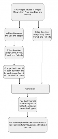
The raw images that are used were varied as follows: image with a small number of edges (image with low frequencies), image with a big number of edges (high-frequency image), image with two kinds of pixel values 0 or 1 (binary image) and the texture image, the edge image for each raw image was found by changing the threshold value until all edges of each image are visible. Those edge images will be used later as a reference [20]. The next step is the noise added to the original images. The noise used is Salt and pepper and the Gaussian noise, then the edge images were found for the noisy images whose correlation values to the raw edge images are as high as possible [21]. Everything has been repeated, but this time by gradually increasing the degree of noise in both Gaussian and Salt and Pepper noise types. Figure 1 shows the methodology flowchart, making the whole idea faster to understand [22].
Figure 1. Methodology flowchart
The results in this paper are not much different from the results of the previous researchers, especially since the issue of finding edges in images is one of the topics researchers have discussed. However, the difference that occurred here, thousands of samples were taken and tested on a bunch of classic edge algorithms. These algorithms are classical algorithms, but even if the threshold of the algorithm is chosen correctly, it still may not give good results. As it is known, the threshold value for the algorithm changes according to the image entered by the algorithm and factors such as noise affecting the image, change in the illumination intensity of the image, and even different capture angles [23, 24].
In this paper is that four famous classical algorithms were tested on several types of images by holding different frequencies and adding different types of noise to them, this generated many data. The number of images reached 50 thousand images in total, and this allowed the experiment of these algorithms on a big number of images [25].
Many possibilities to know how those algorithms perform in different types of images, and with each image, the value of the threshold is changed a thousand times from 0 to 1 with a degree of 0.001, and the values of the threshold that give high correlation values are recorded and saved [26]. This huge work is done by fast GPU because it takes much time to get the final results. The following Table 1 shows the threshold values of the raw edge images, the threshold values of the noisy edge images, and the correlation between the raw edge images and the noisy edge images.
Table 1. Threshold values of the raw images
|
Input |
Edge algorithm |
|||
|
Canny |
Sobel |
Prewitt |
Roberts |
|
|
Binary image |
0.30 |
0.20 |
0.20 |
0.30 |
|
High Freq. image |
0.33 |
0.10 |
0.12 |
0.10 |
|
Low Freq. image |
0.32 |
0.10 |
0.11 |
0.10 |
|
Texture image |
0.35 |
0.35 |
0.35 |
0.35 |
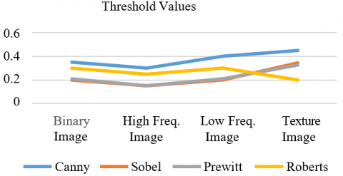
Figure 2 shows that the highest threshold values were with the Canny edge detection algorithm, and in the case of the texture input image, the threshold values obtained in all types of edge detection algorithms are high compared to other types of images. Edge determination is used the Canny algorithm, which has several working steps that make it different from the rest of the other algorithms. The steps are noise reduction, gradient computation, non-maximum suppression, use of two thresholds, and edge tracking. These steps, in particular the step of using two thresholds, make the threshold values slightly larger than the rest of the algorithms, arguably starting from 0.3.
It manually checked the threshold and optimized the code based on the result of the Gaussian noise optimization. The ground truth noise detection samples are proposing the Canny algorithm in the paper is highly responsive in comparison with the existing Sobel, Prewitt, and Roberts algorithms. The Mean-Square-Error (MSE) which is representing the cumulative squared error between the noisy image instance and the original image demonstrates that the optimization of the proposed algorithm is showing a distinguished novelty in the case of computational mechanism.
Figure 2. Threshold values of the raw images
Table 2. Threshold values - gaussian noise
|
Input |
Edge algorithm |
|||
|
Canny |
Sobel |
Prewitt |
Roberts |
|
|
Binary image |
0.35 |
0.20 |
0.21 |
0.30 |
|
High Freq. image |
0.30 |
0.15 |
0.15 |
0.25 |
|
Low Freq. image |
0.40 |
0.20 |
0.21 |
0.30 |
|
Texture image |
0.45 |
0.35 |
0.33 |
0.20 |
So just like the images that did not contain noise, here for the noisy Gaussian Images, the previous Table 2 and Figure 3 show that the highest threshold values were with the Canny edge detection algorithm, and in the case of the texture input image, the threshold values were obtained in all types of the edge detection algorithms was high compared to other types of images [27].
Figure 3. Threshold values of the gaussian noisy edge images
The texture input image is known to all that this image consists of low and high frequencies more than other images. If it cut the image into several small pieces, each piece will consist of a group of high and low frequencies, in other words, this type of image has a sharper and more sudden gradation than the rest of the image types.
The work will be within the lower and higher frequencies more than the rest of the frequencies and is exactly made the values of all the thresholds for all algorithms close in this type of image. Moreover, the threshold values for both Sobel and Prewitt were almost the same.
Table 3. Threshold values – salt and pepper noise
|
Input |
Edge algorithm |
|||
|
Canny |
Sobel |
Prewitt |
Roberts |
|
|
Binary image |
0.35 |
0.26 |
0.25 |
0.30 |
|
High Freq. image |
0.30 |
0.15 |
0.15 |
0.10 |
|
Low Freq. image |
0.42 |
0.12 |
0.10 |
0.10 |
|
Texture image |
0.45 |
0.40 |
0.43 |
0.45 |
Table 3 shows high values of binary images, high frequencies images, low frequencies images, and texture images. Also, it already gave the same results Canny, Sobel, Prewitt, and Roberts in texture images. Salt & pepper noise is one of the types of noise in the image. De-noising is a process of removing and limiting the effect of noise in the image, which helps in better interpretation and analysis of the image.
With the salt and pepper noise edge detection, the above Table 3 and Figure 4, the heights threshold values were with Canny edge detection, also the results of Sobel, Roberts and Prewitt were close.
Figure 4. Threshold values of the salt and pepper noisy edge images
Table 4. Correlation values – Gaussian noise
|
Input |
Edge algorithm |
|||
|
Canny |
Sobel |
Prewitt |
Roberts |
|
|
Binary image |
0.98 |
0.96 |
0.96 |
0.97 |
|
High Freq. image |
0.75 |
0.65 |
0.65 |
0.55 |
|
Low Freq. image |
0.6 |
0.45 |
0.45 |
0.25 |
|
Texture image |
0.99 |
0.60 |
0.60 |
0.98 |
Figure 5. Correlation Gaussian noisy edge images / raw edge images
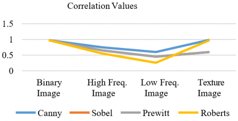
The above Table 4 and Figure 5 clearly show the highest correlation values with the Canny edge detection in all types of images. Moreover, as it is known that the correlation values are between - 1 and 1, whenever the value is close to 1, the correlation is very strong, and if the value is 0, there is no correlation, and in the case of a -1, that means they are opposite.
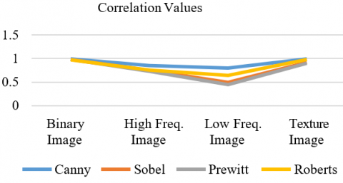
It is clear from Table 5 and Figure 6 that correlation values are all high with the Canny edge detection algorithm and with the image of a type of texture with all kinds of edge detection algorithms. The correlation value of the binary image added by salt and pepper noise with threshold 0.35 in Table 3, its edge found with Canny edge algorithm is 0.99 in Table 5, and so on for the other values.
All edge detection worked so well when the input was a binary image; see the correlation tables. The pixel probability here is either 0 or 1, so there are no other possibilities. See Table 4, Table 5, Figure 5, and Figure 6.
Table 5. Correlation values – salt and pepper noise
|
Input |
Edge algorithm |
|||
|
Canny |
Sobel |
Prewitt |
Roberts |
|
|
Binary image |
0.99 |
0.98 |
0.98 |
0.97 |
|
High Freq. image |
0.85 |
0.75 |
0.73 |
0.76 |
|
Low Freq. image |
0.80 |
0.50 |
0.45 |
0.65 |
|
Texture image |
0.99 |
0.92 |
0.90 |
0.98 |
Figure 6. Correlation salt and pepper noisy edge images / raw edge images
When the input was a texture image, Robert’s edge detection did the best here; see the correlation tables, and this is because the synthesis of the texture image is more compatible with Robert's operators. Table 4, Table 5, Figure 5, and Figure 6. inform this.
For all algorithms, the performance was not so good in the case of the image that contains a huge number of edges. See the correlation tables for the high-frequency image. The possibilities of the edge here are many, leading to taking some of the image pixels and treating them as not edge pixels, which may be the opposite. See Table 4, Table 5, Figure 5, and Figure 6.
For all cases, the threshold values range for the Canny edge detection was from 0.30 to 0.45. This range is the most suitable for all images, and this is what is done here. It is known that the threshold values are from 0 to 1. This study's main subject is finding the best threshold values that make the edge algorithm give the best edge detection. See Table 1, Table 2, Table 3, Figure 2, Figure 3, and Figure 4.
The threshold values of Sobel and Prewitt algorithms were close to each other; see the threshold tables. The operators of Prewitt and Sobel are similar and are used to detect the vertical and horizontal edges. Check it out in Table 1, Table 2, Table 3, Figure 2, Figure 3, and Figure 4.
For Roberts, Sobel, and Prewitt edge detection algorithms, the range of the threshold values was from 0.1 to 0.45; see the threshold tables. So, this range is the most suitable for all images. Moreover, this study's main subject is finding the best threshold values that make the edge algorithm give the best edge detection. See Table 1, Table 2, Table 2, Figure 2, Figure 3, and Figure 4.
Canny edge detection is demonstrating a good result based on the threshold and Mean Square Error (MSE) computation in all cases of input images, even if the noise degree was high and with a randomly modified seed. All edge detection algorithms had a good result for the input type Binary image. For the input type texture image, it is good to use Robert's edge detection algorithm. All edge detection algorithms face difficulties if the input image contains many edges. The canny edge detection threshold range was from 0.30 to 0.45. Sobel and Prewitt's algorithms had a close result to each other. For Roberts, Sobel, and Prewitt's edge detection algorithms, the range of the threshold values was from 0.1 to 0.45. In this article, four famous classical algorithms have been tested on many types of frames by keeping different frequencies and adding different types of noise to them, it produces a lot of data because the total frames reach 50,000 frames, this allows testing of these algorithms on a large number of images. Among the four algorithms used, the Canny algorithm proved the best in all input cases. It came following Bin and Yeganeh [16], Chandrasekar and Shrivakshan [17], and Maini and Aggarwal [10], and this is because this algorithm makes smoothing to the input image due to the Gaussian filter that it has, calculates the gradient depending on the gradient of Sobel or Prewitt, and find the image edge by using the non-maximum suppression and connect the thresholding based on the hysteresis [28, 29]. A large number of possibilities to know how those algorithms perform in different types of images, and with each image, the value of the threshold is changed a thousand times from 0 to 1 with a degree of 0.001, and the values of the threshold that give high correlation values are recorded and saved. This huge work is done by fast GPU because it takes much time to get the final results. This study is important in terms of setting an example for future studies in terms of edge detection. In addition, which algorithms and methods used are more important are given comparatively. This will shed light on future researchers.
[1] Gonzalez, R.C. (2009). Digital image processing. Pearson Education India, 572-585.
[2] Reddy, S.P.K., Harikiran, J. (2022). Cast Shadow Angle Detection in morphological aerial images using faster R-CNN. Traitement du Signal, 39(4): 1313-1321. https://doi.org/10.18280/ts.390424
[3] Jing, J., Liu, S., Wang, G., Zhang, W., Sun, C. (2022). Recent advances on image edge detection: A comprehensive review. Neurocomputing, 533: 259-271. https://doi.org/10.1016/j.neucom.2022.06.083
[4] Chen, C.C. (1977). Fast boundary detection: A generalization and a new algorithm. IEEE Transactions on Computers, 100(10): 988-998. https://doi.org/10.1109/TC.1977.1674733
[5] Canny, J. (1986). A computational approach to edge detection. IEEE Transactions on Pattern Analysis and Machine Intelligence, (6): 679-698. https://doi.org/10.1109/TPAMI.1986.4767851
[6] Bi, Y., Xue, B., Mesejo, P., Cagnoni, S., Zhang, M. (2022). A survey on evolutionary computation for computer vision and image analysis: Past, present, and future trends. arXiv preprint arXiv: 2209.06399.
[7] Tang, S. (2000). Survey of Edge Detection. tang-s@ cs.unr.edu.
[8] Woods, J.W., Ekstrom, M.P. (1984). Image detection and estimation. Digital Image Processing Techniques, 2: 77.
[9] Maini, R., Sohal, J.S. (2006). Performance evaluation of Prewitt edge detector for noisy images. GVIP Journal, 6(3): 39-46.
[10] Maini, R., Aggarwal, H. (2009). Study and comparison of various image edge detection techniques. International Journal of Image Processing (IJIP), 3(1): 1-11.
[11] Rode, K.N., Siddamallaiah, R.J. (2022). Image segmentation with priority based apposite feature extraction model for detection of multiple sclerosis in MR images using deep learning technique. Traitement du Signal, 39(2): 763-769. https://doi.org/10.18280/ts.390242
[12] Nandhitha, N.M., Manoharan, N., Rani, B.S., Venkataraman, B., Raj, B. (2006). A comparative study on the performance of the classical and wavelet-based edge detection for image denoising on defective weld thermographs. In Asia Pacific Conference on NDT.
[13] Luo, W. (2006). Comparison for edge detection of colony images. IJCSNS International Journal of Computer Science and Network Security, 6(9A): 211-215.
[14] Nadernejad, E., Sharifzadeh, S., Hassanpour, H. (2008). Edge detection techniques: Evaluations and comparisons. Applied Mathematical Sciences, 2(31): 1507-1520.
[15] Joshi, S.R., Koju, R. (2012). Study and comparison of edge detection algorithms. IEEE Internet, Third Asian Himalayas International Conference, pp. 23-25. https://doi.org/10.1109/AHICI.2012.6408439
[16] Bin, L., Yeganeh, M.S. (2012). Comparison for image edge detection algorithms. IOSR Journal of Computer Engineering, 2(6): 1-4.
[17] Shrivakshan, G.T., Chandrasekar, C. (2012). A comparison of various edge detection techniques used in image processing. International Journal of Computer Science Issues (IJCSI), 9(5): 269.
[18] Rafael, C.G., Richard, E.W. (2002). Digital Image Processing. 2nd edition, Prentice Hall.
[19] Mather, P.M. (1986). Review of: “Introductory Digital Image Processing: A Remote Sensing Perspective” By JR JENSEN:(Englewood Cliffs, New Jersey: Prentice Hall, 1986)[Pp. 368.] Price£ 53-45. International Journal of Remote Sensing, 7(12): 1836-1838. https://doi.org/10.1080/01431168608948975
[20] Marr, D., Hildreth, E. (1980). Theory of edge detection. Proceedings of the Royal Society of London. Series B. Biological Sciences, 207(1167): 187-217. https://doi.org/10.1098/rspb.1980.0020
[21] Karanwal, S. (2021). Implementation of edge detection at multiple scales. Int. J. Eng. Manuf, 11(1): 1-10. https://doi.org/10.5815/ijem.2021.01.01
[22] Sharifi, M., Fathy, M., Mahmoudi, M.T. (2002). A classified and comparative study of edge detection algorithms. In Proceedings. International conference on information technology: Coding and computing, IEEE, pp. 117-120. https://doi.org/10.1109/ITCC.2002.1000371
[23] Abbasi, T.A., Abbasi, M.U. (2007). A novel FPGA-based architecture for Sobel edge detection operator. International Journal of Electronics, 94(9): 889-896.
[24] Matthews, J. An introduction to edge detection. The sobel edge detector. http://www/generation5.org/content/2002.im01.im01.asp, accessed on Sep. 17, 2022.
[25] Davies, E.R. (1986). Constraints on the design of template masks for edge detection. Pattern Recognition Letters, 4(2): 111-120. https://doi.org/10.1016/0167-8655(86)90032-2
[26] Chen, C.C. (1977). Fast boundary detection: A generalization and a new algorithm. IEEE Transactions on Computers, 100(10): 988-998. https://doi.org/10.1109/TC.1977.1674733
[27] Haralick, R.M. (1987). Digital step edges from zero crossing of second directional derivatives. In Readings in Computer Vision, Morgan Kaufmann, pp. 216-226. https://doi.org/10.1016/B978-0-08-051581-6.50027-1
[28] Canny, J. (1986). A computational approach to edge detection. IEEE Transactions on Pattern Analysis and Machine Intelligence, (6): 679-698. https://doi.org/10.1109/TPAMI.1986.4767851
[29] Datta, A. (2009). Removal of random valued impulsive noise. Doctoral dissertation. Department of Computer Science and Engineering, National Institute of Technology Rourkela.