Ke Wang | Ying An | Ni Li | Jiancun Zhou | Xianlai Chen*
© 2022 IIETA. This article is published by IIETA and is licensed under the CC BY 4.0 license (http://creativecommons.org/licenses/by/4.0/).
OPEN ACCESS
Identifying the histological phenotype of non-small cell lung cancer (NSCLC) is of crucial importance to its treatment and prognosis. The radiomics-based prediction model has the potential to non-invasively extract the tumor phenotype characteristics. However, the existing research ignores the stability of extracted features, which restricts the performance and robustness of the constructed model. While most of themethods in the literature use classification accuracy to solve theproblemofradiomics featuresstability, in this paper we propose the use ofSOM (Self-organizing Mapping) and K-means to evaluate the stability of different feature subsets. The subset with good clustering performance is selected as the optimal feature subset.When the optimal feature subset is used for modeling, compared with other feature subsets, the higher AUC(Area Under Curve) and lower SD(Standard Deviation) on the three classifiers show that the feature subset had excellent classification performance and good stability, and can distinguish NSCLC subtypes more accurately and robustly.
non-small cell lung cancer, radiomics, feature extraction, SOM network, robust identification
In many countries, lung cancer is the main cause of cancer-related death. In particular, lung cancer is the most common cancer type in China, which induces over 430,000 deaths annually [1]. Typically, non-small cell lung cancer (NSCLC) accounts for approximately 85% of lung cancer [2]. The rate of cancer proliferation and diffusion of NSCLC are relatively slow, and the early symptoms are not obvious. The vast majority of NSCLC patients are in the middle and late when they are diagnosed [3], and lost the opportunity of surgical treatment. Neoadjuvant chemotherapy (NACT) is the preferred choice for patients with inoperable stage III / IV NSCLC, but different NSCLC subtypes have different sensitivity to NACT drugs. For instance, Antifolate Pemetrexed-based chemotherapy is only effective on lung adenocarcinoma (ADC), while Bevacizumab is recommended for squamous cell carcinoma of lung (SCC) [4-6]. Therefore, determining the NSCLC histological subtypes contributes to formulating the correct treatment strategies and avoids the chemotherapy-related side effects [7]. At present, pathological diagnosis is the gold standard to distinguish SCC and ADC [8], but it requires invasive biopsy, while aspiration biopsy may bring the risk of massive bleeding in patients with advanced lung cancer. Therefore, it is urgently needed to develop a non-invasive method to accurately classify lung cancer subtypes, thus providing the more appropriate diagnosis and treatment strategy for the patients, which is of great significance to maximally prolong the survival of patients.
Radiomics analysis is an emerging quantitative analysis method, which can automatically, efficiently and repeatedly extract the mass, objective and indiscernible tumor features from medical images (such as CT, MRI and PET), and mine the potential relationships between quantitative image features and pathophysiological features. Radiomics analysis can be used to predict diverse clinical outcomes, such as survival, distant metastasis (DM) and molecular feature classification [9-13]. Some studies focus on the radiomics-based identification of NSCLC histological subtypes. Wu et al. [14] constructed two study cohorts (training and validation cohort) involving altogether 350 patients, and 440 radiomics features based on CT images were extracted from each sample. Han et al. [15] retrospectively studied 129 NSCLC patients and extracted 485 features from the artificially labeled tumor region. They constructed the radiomics-based model by the logistic regression, and the AUC of the model was 0.893 (95% CI: 0.789 to 0.996). Chaunzwa et al. [16] retrospectively studied 157 patients with NSCLC to classify ADC or SCC. They used a VGG-16 neural network to extract deep features from CT images and classify them with fully connected layers, and its AUC were high (0.751). Although these studies have achieved favorable achievements, the research on the classification of NSCLC subtypes mainly focuses on the performance of the classifier, and there is less research on the stability of feature selection. When the training data changes slightly, the difference of the optimal feature subset changes greatly, and the prediction accuracy of the classification model is greatly biased. These have reduced stability of the models and restricted its clinical application. Therefore, it is necessary to explore methods improving feature stability to enhance robustness of the model.
This study collected CT and clinical data from Yiyang Central Hospital and extracted radiomics features from the CT image data. Several feature subsets were selected by LASSO. The SOM and K-means were used to evaluate the classification performance of each feature subset, and the feature subset with good performance was selected as the optimal subset. In order to verify the results generated by SOM and K-means, logistic regression (LR), support vector machine (SVM) and random forest (RF) classification models were constructed to evaluate the performance of feature subset.
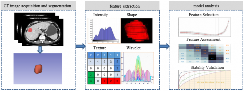
The workflow of this study was shown as Figure 1, including such steps as CT image acquisition and segmentation, feature extraction, model analysis.
2.1 Collecting and preprocessing of data
Altogether 163 ADC and SCC patients, who admitted and treated in Yiyang Central Hospital from January 2016 to December 2020, were collected. The inclusion criteria were as follows, (1) CT images before treatment can be obtained; (2) the postoperative pathology verified ADC or SCC. After excluding 15 cases who received surgery in other hospitals and 10 cases without pathological results, 138 cases were finally enrolled for analysis. Then the enrolled patients were sorted according to the time of diagnosis and randomly split as training set (n=110) and validation set (n=28) at a ratio of 8:2. Among all the enrolled patients, there were 83 ADC cases and 55 SCC cases, with the age of 44-83 (median, 65) years. Meanwhile, there were 104 male and 34 female cases. The patient characteristics are displayed in Table 1.
Table 1. Summary of patient characteristics
|
|
ADC |
SCC |
|
age |
|
|
|
range(median) |
44~83(65) |
45~82(66) |
|
mean + std |
64.3+8.7 |
65.2+8.2 |
|
gender |
|
|
|
male |
50 |
54 |
|
female |
33 |
1 |
Pulmonary CT examinations were performed using four CT scanners, with the tube voltage of 120 kVp, tube current of 220 mAs, and interlayer thickness of 4-5 mm. The CT images of each patient were analyzed by an experienced radiologist (with 8 years of experience) by using the medical imaging interactive package (3DSlicer) (20210226 edition; https://download.slicer.org//), and validated by another experienced radiologist (with 15 years of experience). Any different interpretations between them were dissolved by group discussion to finally reach consensus.
2.2 Extracting and selecting of feature
Using the pyradiomics software (Version 2.1.2, https://github.com/Radiomics/pyradiomics.git), A large number of radiomics features were extracted from the region of interest (ROI) to quantify the NSCLC images, including the tumor intensity, shape, size, texture and wavelet features [17, 18]. Nonetheless, too many features will increase the computational expenses, and the redundancy of features will reduce the classification accuracy. Moreover, the feature number in this study was greater than the sample number, which increased the probability of overfitting. Therefore, feature selection is of crucial importance. LASSO was the most commonly used techniques for feature selection in radiomics [19-23]. Here LASSO regression was used to select the radiomics features closely related to subtypes. It constructs a penalty function to compress the regression coefficient, which can reduce the coefficients of corresponding features to zero. Since each coefficient is associated with a feature, so feature selection is achieved by retaining features with non-zero coefficients [24]. LASSO increases a L1 regular term on the traditional linear regression model, and its target loss function becomes:
$J(\omega)=\min \left\{\frac{1}{2 N}\left\|X^T \omega-y\right\|_2^2+\alpha\|\omega\|\right\}$ (1)
where, N is the sample number, X is the sample, y is the label of the sample, ||ω|| is the L1 norm, α stands for the constant coefficient that controls the penalty degree of spare estimation, and the optimal α can be selected depending on cross validation and information criteria. Model selection based on information criteria depends on the model hypothesis, and the model sample size should be appropriately estimated. As a result, when the feature number is far greater than the sample size, the feature selection effect of this method will significantly decrease. As for high-dimensional feature data with correlations among variables, cross validation can not only achieve a high computational efficiency, but also has a better effect.
Figure 1. Workflow of this study
2.3 Features evaluation
When the training sets were changed, the feature subset selected by the same feature selection algorithm was different. To be brief, there was more than one feature subset. In this paper, two unsupervised methods were used to evaluate the feature stability. They can rely on the sample feature information to explore and reveal the potential structure and distribution law of the data set itself, that was, the samples with similar features were gathered into a group, and the samples in different groups had highly different characteristics. If there was a stable feature subset, there would be good clustering performance.
SOM network is an unsupervised algorithm proposed by Kohonen, which can reveal the complicated non-linearity hidden in the high-dimensional data, and display the relationships between samples in the low-dimensional space in a visual manner while maintaining the original spacial topological relation [25]. Suppose the input layer X=(x1, x2, xn) is an N-dimensional vector, the output layer is a two-dimensional network with M nodes, and Wijis the weight between the ith input neuron node and the jth output neuron node. The training steps of the algorithm are as follows:
Step 1: Initialization: Randomly initializes node parameters. The number of parameters in each node is the same as the input dimension;
Step 2: Randomly select sample X and calculate the distance between X and the output node, denoted by d(x, w);
$\mathrm{d}(\mathrm{x}, \mathrm{w})=\sqrt{\sum_{i=1}^{\mathrm{n}}\left(\mathrm{x}_{\mathrm{i}}-\mathrm{w}_{ij}\right)^2}$ (2)
Step 3: The node with the smallest distance was selected as the winner node;
Step 4: Calculate the node update amplitude according to the neighborhood function h(i, j), the node close to the winning neuron has a large weight wij update;
$h(i, j)=e^{-\frac{\left(c_x-i\right)^2}{2 \delta^2}} e^{-\frac{\left(c_y-j\right)^2}{2 \delta^2}}$ (3)
where, (cx, cy) is the winner node;
Step 5: Update the weights of nodes in the neighborhood;
$\mathrm{w}_{i j}(\mathrm{t}+1)=\mathrm{w}_{\mathrm{ij}}(\mathrm{t})+\alpha(\mathrm{t}) \mathrm{h}(\mathrm{i}, \mathrm{j})\left[\mathrm{x}(\mathrm{t})-\mathrm{w}_{i j}(\mathrm{t})\right]$ (4)
$\alpha(\mathrm{t})=\alpha\left(\mathrm{t}_0\right) /\left(1+\mathrm{t} / \max _{\mathrm{step}}\right)$ (5)
where, α(t) is the initial learning rate, $\max _{s t e p}$ is the maximum number of iterations, and t is the current times of iterations;
Step 6: Repeat the above steps until the set number of iterations is met.
After several iterations, the optimal SOM model is finally established. The model can map the test samples to the two-dimensional plane, so that the same classification of data is gathered, different classification of data is separated, and the topology of the data set remains unchanged. The feature subset with good clustering result shows that it can distinguish different classification samples well.
K-means adopts distance as the evaluation criterion of similarity, that is, the closer the distance between two objects is, the greater the similarity will be. This algorithm considers that clusters are composed of objects that are close to each other, so the ultimate goal is to obtain compact and independent clusters. The algorithm flow is as follows:
Step 1: Two points are selected as cluster centers of initial aggregation;
Step 2: The Euclidean distance is used to calculate the distance from each sample point to the two cluster cores, find the cluster center nearest to the point, and assign it to the corresponding cluster;
Step 3: After samples points are grouped into clusters, the M samples are divided into 2 clusters. Then the center of gravity of each cluster is recalculated as the new "cluster center";
Step 4: Repeat steps 2-3 until the set number of iterations is met.
K-means algorithm is simple and efficient. The clustering results can also be used to evaluate the stability of feature subsets. Compared with SOM network, k-means only updates the parameters of this cluster after finding the most similar cluster for each input data, while SOM updates all nodes in the neighborhood, so K-means is more affected by noise. When the number of features is greater than 2, it is not suitable for visualization.
2.4 Constructing of classifiers
In order to verify the results generated by SOM and k-means. Three classification algorithms were adopted here, including logistic regression (LR), support vector machine (SVM) and random forest (RF), to classify SCC and ADC in NSCLC. LR is a classical machine learning algorithm, which is usually used in the binary classification task and model view estimated probability p (y=1 | x), namely, the probability at y=1 under the given data x. The advantages of LR include the rapid training speed and the suitability of using discrete variables and continuous variables as the inputs. Nonetheless, its disadvantage is that it cannot achieve satisfactory classification effect for complicated data as a linear model. However, the LR model attains favorable effects on numerous datasets, which can be easily realized and can be used as a basic modeling method [26, 27]. SVM is another extensively utilized classification algorithm, which attempts to calculate the decision-making boundary to separate data. This decision boundary, also called the hyperplane, is orientated in such a way that it is as far away as possible from the closest data points (support vectors) from each class [28]. The RF classifier utilizes the bootstrap resampling method to extract multiple samples from the original samples, constructs a decision-making tree for each bootstrap sample, and finally combines all the decision-making trees to obtain the final classification result [29, 30].
3.1 The extracted and selected features
Altogether 857 features were extracted from the tumor region of each sample. When LASSO was used in feature selection, different feature subsets can be obtained by randomly selecting training sets from the data set for many times. For each random training set, in order to obtain the feature subset with the best classification performance, the grid search was adopted for determining the optimal hyper-parameters values.
In Figure 2, the LASSO was adopted to select 9 radiomics features with non-zero coefficients from the 857 radiomics features to form a feature subset, which was represented by FS_A. The vertical line in Figure 2(A) represents the alpha value selected after 10-fold cross-validation. Figure 2(B) indicates the feature importance.
Where F1, F2...F9 represent different features, respectively, as shown in Table 2.
Figure 2. Feature subsets were selected by LASSO
Table 2. Feature importance and weight of FS_A
|
Id |
Feature name |
Weight |
|
F1 |
wavelet-HHLfirstorderMinimum |
-0.11 |
|
F2 F3 F4 F5 F6 F7 |
wavelet-HLLfirstorderTotalEnergy wavelet_LHLfirstorderEnergy wavelet-LLLfirstorderMedian originalshapeSphericity wavelet-LLHglrlmLongRunLowGrayLevelEmphasis wavelet-HHHgldmLargeDependenceLowGrayLevelEmphasis |
-0.08 -0.07 -0.06 -0.06 0.04 0.05 |
|
F8 F9 |
wavelet-LLLglcmContrast wavelet-HHHglrlmRunVariance |
0.07 0.08 |
Table 3. Feature importance and weight of FS_B
|
Id |
Feature name |
Weight |
|
F1 |
wavelet-LHHfirstorderEnergy |
-0.07 |
|
F2 F3 F4 F5 F6 F7 |
wavelet-LLLfirstorderMedian wavelet-HLLfirstorderTotalEnergy wavelet-HLLngtdmStrength wavelet-HHHgldmLargeDependenceLowGrayLevelEmphasis wavelet-LLLglcmContrast wavelet-LLHglrlmLongRunLowGrayLevelEmphasis |
-0.03 -0.01 0.01 0.03 0.05 0.05 |
Figure 3. Visualize samples of different features subset using the SOM network. (A) Visualize samples of FS_A, (B) Visualize samples of FS_B
The training set is changed randomly for many times, and different feature subset was obtained by LASSO. While feature weights were not taken into account, only one feature subset was different from the previous FS_A, which was represented by FS_B. A group of weights was randomly selected in FS_B, and the importance and weight of its features were shown in Table 3, Where F1, F2...F7 represent different features, respectively.
3.2 Evaluate features subsets
As you can see from the previous section, different training sets can select different subsets of features when using LASSO. Two unsupervised algorithms are used to evaluate the stability of feature subsets.
In Figure 3(A), SCC and ADC samples were concentrated in different regions, and there were less mixed samples. Compared with Figure 3(A), there were more mixed samples in Figure 3(B).
Table 4. AUC in unsupervised learning
|
Feature subset |
SOM |
K-means |
|
FS_A |
0.77 |
0.65 |
|
FS_B |
0.58 |
0.57 |
The accuracy of SOM and K-means was used to evaluate the clustering performance of FS_A and FS_B, as shown in Table 4. The AUC of FS_A was better than FS_B. It can be suggested that FS_A exhibited higher discrimination than FS_B and that FS_A is considered as the best feature subset. Secondly, k-means was affected by noise data, and the clustering performance was slightly worse.
3.3 The prediction model using the machine learning algorithm
As mentioned in the previous section, FS_A was the optimal feature subset. The following three machine learning methods were used to verify it. For each method, the optimal hyper-parameter was selected by grid search and 10-fold cross validation. According to the previously selected feature subsets, three classifiers were used to modeling and analyzing, respectively. In addition, the AUC was used to evaluate classification of the model, and SD of AUC was employed to evaluate stability of the model. Among 10 different training sets, the classification performance and stability of FS_A and FS_B in LR, RF and SVM models was shown as Table 5.
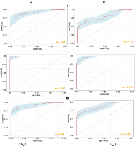
It can be seen from table 5 that the training set was changed, and the prediction model based on FS_A has high AUC and low SD. When modeling with the first training set, the performance of the models was shown as Figure 4. I, II and III represent respectively the AUC values in the models by LR, RF, SVM.
The red line represents ROC, and the shadow stands for the corresponding 95% CI. A smaller shadow area suggests the less AUC fluctuation and the more stable prediction model. It was observed that the AUC of the RF model was the highest among all models. As shown in Figure 4, FS_A had a larger AUC and a smaller shadow area than the corresponding FS_B. The results of three models show that the model based on FS_A had good classification performance and stability.
3.4 Discussion
SCC and ADC are two types of most common NSCLC, which share similar clinical manifestations, but their treatment strategies and prognostic outcomes are greatly different. Therefore, accurate subtype discrimination is the essential step to formulate the reasonable and effective treatment strategies and to prolong patient lifespan. The radiomics model was constructed based on lung CT images, which was used to identify SCC and ADC in NSCLC by a non-invasive, accurate and reliable manner. The curse of dimensionality is a huge challenge in the radiomics analysis, so feature selection is an essential step. LASSO is the most commonly used feature selection technology, which is very suitable for dimensionality reduction of radiomics [31, 32]. Therefore, LASSO is selected as the feature dimension reduction method in this paper.
At present, LASSO can select the distinguishing features for the classification of NSCLC subtypes based on radiomics by adjusting parameters, but ignore the problem of feature stability. This stability is ignored, this will reduce model robustness and limit the clinical application of the model. When LASSO is used for feature selection, different feature subsets can be obtained from different training sets. How to distinguish feature subsets with excellent classification performance and good stability from feature selection results is a great challenge. The method to evaluate the stability of feature subsets are usually changed datasets or bootstrap sampling methods, which are relatively simple but time-consuming and laborious. SOM and K-means are both unsupervised clustering methods, which can reveal the inherent nature and rules of data through learning unlabeled training samples. As observed from Figure 3, Compared to FS_B, FS_A can clearly distinguish ADC from SCC in SOM network. In Table 4, FS_A had better clustering performance compared with FS_B using k-means method. It shows that FS_A has good classification performance. In order to verify the results produced by SOM and K-means, three classifiers are used to construct the prediction model with LR, SVM and RF. The experimental results show that all classifiers constructed based on FS_A have high accuracy (Shown as Figure 4). Relate the results of Table 4, the classification accuracy of the SOM network on FS_A and FS_B is closer to the results of the three classifiers compared with k-means. It demonstrates that SOM clustering effect is close to the real sample distribution. It was discovered that the FS_A achieved superior stability to FS_B (Shown as Table 5). The results show that the feature subset evaluated excellent by unsupervised clustering not only has good classification, but also has strong stability. Therefore, the unsupervised clustering can be used as one of the methods to select the optimal feature subset, especially SOM network.
Certain limitations should be noted in this study. First, the ROIs were partitioned manually by the radiologists, while the advanced deep learning-based automatic partitioning algorithm was not used, which might lead to subjective error [33]. Moreover, data in this paper were derived from the same hospital and the scanning parameters were the same [34]. In this regard, larger and multi-center cohorts should be recruited for verification in the future.
Table 5. AUC and SD of different feature subsets
|
Training set |
FS_A |
FS_B |
||||||||||
|
AUC |
SD |
AUC |
SD |
|||||||||
|
LR |
RF |
SVM |
LR |
RF |
SVM |
LR |
RF |
SVM |
LR |
RF |
SVM |
|
|
1 |
0.910 |
0.995 |
0.920 |
0.286 |
0.005 |
0.249 |
0.788 |
0.979 |
0.864 |
0.746 |
0.040 |
0.456 |
|
2 |
0.912 |
0.981 |
0.917 |
0.286 |
0.035 |
0.261 |
0.794 |
0.975 |
0.857 |
0.725 |
0.058 |
0.489 |
|
3 |
0.906 |
0.982 |
0.913 |
0.311 |
0.040 |
0.279 |
0.788 |
0.987 |
0.841 |
0.746 |
0.022 |
0.556 |
|
4 |
0.913 |
0.989 |
0.917 |
0.292 |
0.018 |
0.273 |
0.785 |
0.989 |
0.869 |
0.756 |
0.018 |
0.456 |
|
5 |
0.912 |
0.978 |
0.920 |
0.292 |
0.052 |
0.243 |
0.785 |
0.984 |
0.888 |
0.746 |
0.029 |
0.359 |
|
6 |
0.913 |
0.993 |
0.931 |
0.292 |
0.009 |
0.215 |
0.794 |
0.977 |
0.861 |
0.725 |
0.006 |
0.464 |
|
7 |
0.911 |
0.987 |
0.921 |
0.292 |
0.022 |
0.238 |
0.790 |
0.982 |
0.851 |
0.735 |
0.040 |
0.513 |
|
8 |
0.904 |
0.988 |
0.919 |
0.311 |
0.022 |
0.243 |
0.790 |
0.980 |
0.851 |
0.735 |
0.050 |
0.505 |
|
9 |
0.910 |
0.995 |
0.923 |
0.292 |
0.005 |
0.232 |
0.788 |
0.989 |
0.882 |
0.746 |
0.018 |
0.388 |
|
10 |
0.904 |
0.977 |
0.918 |
0.311 |
0.047 |
0.243 |
0.789 |
0.982 |
0.855 |
0.735 |
0.033 |
0.505 |
Figure 4. AUC and corresponding 95% CI of three classifiers based on FS_A or FS_B
To sum up, the unsupervised clustering methods was used to evaluate the stability of feature subset, and the most stable feature subset was regarded as the optimal subset. Using the optimal feature subset to construct subtype classification model with good robustness and high accuracy can help to guide the clinical decision-making of physicians and realize the individualized diagnosis and treatment for patients.
Supported by Precision Medicine Research Project (Grant No.:2016YFC0901705), National Key R&D Program of China; Radiomics evaluation of neoadjuvant chemotherapy for non-small cell lung cancer based on federal learning (Grant No.: 2022JJ30747); Quality improvement and interpretable fusion method for weak label medical data (Grant No.: 2021JJ30082); the National Science Foundation of Hunan Province. The funder had no role in the design of the study and collection, analysis, and interpretation of data and in writing the manuscript.
[1] Chen, W. (2015). Cancer statistics: updated cancer burden in China. Chinese Journal of Cancer Research, 27(1): 1. https://doi.org/10.3978/j.issn.1000-9604.2015.02.07
[2] Zhu, X., Dong, D., Chen, Z., Fang, M., Zhang, L., Song, J., Tian, J. (2018). Radiomic signature as a diagnostic factor for histologic subtype classification of non-small cell lung cancer. European radiology, 28(7): 2772-2778. https://doi.org/10.1007/s00330-017-5221-1
[3] Petty, T.L. (2001). Early diagnosis of lung cancer. Hospital Practice (1995), 36(5): 9-10.
[4] Garde-Noguera, J., Martin-Martorell, P., De Julián, M., Perez-Altozano, J., Salvador-Coloma, C., García-Sanchez, J., Juan-Vidal, O. (2018). Predictive and prognostic clinical and pathological factors of nivolumab efficacy in non-small-cell lung cancer patients. Clinical and Translational Oncology, 20(8): 1072-1079. https://doi.org/10.1007/s12094-017-1829-5
[5] Di Costanzo, F., Mazzoni, F., Mela, M.M. (2008). Bevacizumab in non-small cell lung cancer. Drugs, 68(6): 737-746.
[6] Fukui, T., Taniguchi, T., Kawaguchi, K., Fukumoto, K., Nakamura, S., Sakao, Y., Yokoi, K. (2015). Comparisons of the clinicopathological features and survival outcomes between lung cancer patients with adenocarcinoma and squamous cell carcinoma. General Thoracic and Cardiovascular Surgery, 63(9): 507-513. https://doi.org/10.1007/s11748-015-0564-5
[7] Yang, F., Chen, W., Wei, H., Zhang, X., Yuan, S., Qiao, X., Chen, Y.W. (2021). Machine learning for histologic subtype classification of non-small cell lung cancer: a retrospective multicenter radiomics study. Frontiers in Oncology, 10: 608598. https://doi.org/10.3389/fonc.2020.608598
[8] Travis, W.D. (2011). Classification of lung cancer. In Seminars in Roentgenology, 46(3): 178-186.
[9] Kumar, V., Gu, Y., Basu, S., Berglund, A., Eschrich, S. A., Schabath, M. B., Gillies, R.J. (2012). Radiomics: the process and the challenges. Magnetic Resonance Imaging, 30(9): 1234-1248. https://doi.org/10.1016/j.mri.2012.06.010
[10] Choi, E.R., Lee, H.Y., Jeong, J.Y., Choi, Y.L., Kim, J., Bae, J., Shim, Y.M. (2016). Quantitative image variables reflect the intratumoral pathologic heterogeneity of lung adenocarcinoma. Oncotarget, 7(41): 67302. https://doi.org/10.18632/oncotarget.11693
[11] Gillies, R.J., Kinahan, P.E., Hricak, H. (2016). Radiomics: Images are more than pictures, they are data. Radiology, 278(2): 563. https://doi.org/10.1148/radiol.2015151169
[12] Aerts, H.J., Velazquez, E.R., Leijenaar, R.T., Parmar, C., Grossmann, P., Carvalho, S., Lambin, P. (2014). Decoding tumour phenotype by noninvasive imaging using a quantitative radiomics approach. Nature Communications, 5(1): 1-9. https://doi.org/10.1038/ncomms5006
[13] Chen, Y., Wang, Y., Cai, Z., Jiang, M. (2021). Predictions for central lymph node metastasis of papillary thyroid carcinoma via CNN-based fusion modeling of ultrasound images. Traitement du Signal, 38(3): 629-638. https://doi.org/10.18280/ts.380310
[14] Wu, W., Parmar, C., Grossmann, P., Quackenbush, J., Lambin, P., Bussink, J., Aerts, H.J. (2016). Exploratory study to identify radiomics classifiers for lung cancer histology. Frontiers in Oncology, 6: 71. https://doi.org/10.3389/fonc.2016.00071
[15] Han, Y., Ma, Y., Wu, Z., Zhang, F., Zheng, D., Liu, X., Guo, X. (2021). Histologic subtype classification of non-small cell lung cancer using PET/CT images. European Journal of Nuclear Medicine and Molecular Imaging, 48(2): 350-360. https://doi.org/10.1007/s00259-020-04771-5
[16] Chaunzwa, T.L., Christiani, D.C., Lanuti, M., Shafer, A., Diao, N., Mak, R.H., Aerts, H. (2018). Using deep-learning radiomics to predict lung cancer histology. Journal of Clinical Oncology, 36(15): 8545-8545.
[17] Liang, Z.G., Tan, H.Q., Zhang, F., Rui Tan, L.K., Lin, L., Lenkowicz, J., Kiang Chua, M.L. (2019). Comparison of radiomics tools for image analyses and clinical prediction in nasopharyngeal carcinoma. The British Journal of Radiology, 92(1102): 20190271. https://doi.org/10.1259/bjr.20190271
[18] Gao, X., Ma, T., Bai, S., Liu, Y., Zhang, Y., Wu, Y., Ye, Z. (2020). A CT-based radiomics signature for evaluating tumor infiltrating Treg cells and outcome prediction of gastric cancer. Annals of Translational Medicine, 8(7): 469-469. https://doi.org/10.21037/atm.2020.03.114
[19] Shen, C., Liu, Z., Wang, Z., Guo, J., Zhang, H., Wang, Y., Tian, J. (2018). Building CT radiomics based nomogram for preoperative esophageal cancer patients lymph node metastasis prediction. Translational Oncology, 11(3): 815-824. https://doi.org/10.1016/j.tranon.2018.04.005
[20] Shen, C., Liu, Z., Guan, M., Song, J., Lian, Y., Wang, S., Tian, J. (2017). 2D and 3D CT radiomics features prognostic performance comparison in non-small cell lung cancer. Translational Oncology, 10(6): 886-894. https://doi.org/10.1016/j.tranon.2017.08.007
[21] Ma, C., Huang, J. (2016). Asymptotic properties of Lasso in high-dimensional partially linear models. Science China Mathematics, 59(4): 769-788. https://doi.org/10.1007/s11425-015-5093-2
[22] Steyerberg, E.W. (2016). FRANK E. HARRELL, Jr., Regression Modeling Strategies: With Applications, to Linear Models, Logistic and Ordinal Regression, and Survival Analysis, 2nd ed. Heidelberg: Springer. Biometrics, 72(3): 1006-1007. https://doi.org/10.1111/biom.12569
[23] Song, J., Yin, Y., Wang, H., Chang, Z., Liu, Z., Cui, L. (2020). A review of original articles published in the emerging field of radiomics. European Journal of Radiology, 127: 108991. https://doi.org/10.1016/j.ejrad.2020.108991
[24] Alvarez-Jimenez, C., Sandino, A.A., Prasanna, P., Gupta, A., Viswanath, S.E., Romero, E. (2020). Identifying cross-scale associations between radiomic and pathomic signatures of non-small cell lung cancer subtypes: Preliminary results. Cancers, 12(12): 3663. https://doi.org/10.3390/cancers12123663
[25] Nasief, H., Zheng, C., Schott, D., Hall, W., Tsai, S., Erickson, B., Allen Li, X. (2019). A machine learning based delta-radiomics process for early prediction of treatment response of pancreatic cancer. NPJ Precision Oncology, 3(1): 1-10. https://doi.org/10.1038/s41698-019-0096-z
[26] Forghani, R., Savadjiev, P., Chatterjee, A., Muthukrishnan, N., Reinhold, C., Forghani, B. (2019). Radiomics and artificial intelligence for biomarker and prediction model development in oncology. Computational and Structural Biotechnology Journal, 17: 995.
[27] Örnek, A.H., Ervural, S., Ceylan, M., Konak, M., Soylu, H., Savaşçı, D. (2020). Classification of medical thermograms belonging neonates by using segmentation, feature engineering and machine learning algorithms. Traitement du Signal, 37(4): 611-617. https://doi.org/10.18280/ts.370409
[28] Huang, S., Cai, N., Pacheco, P.P., Narrandes, S., Wang, Y., Xu, W. (2018). Applications of support vector machine (SVM) learning in cancer genomics. Cancer Genomics & Proteomics, 15(1): 41-51.
[29] He, B., Ji, T., Zhang, H., Zhu, Y., Shu, R., Zhao, W., Wang, K. (2019). MRI‐based radiomics signature for tumor grading of rectal carcinoma using random forest model. Journal of Cellular Physiology, 234(11): 20501-20509. https://doi.org/10.1002/jcp.28650
[30] Özel, E., Tekin, R., Kaya, Y. (2021). Implementation of artifact removal algorithms in gait signals for diagnosis of parkinson disease. Traitement du Signal, 38(3): 587-597. https://doi.org/10.18280/ts.380306
[31] Sun, Y., Li, C., Jin, L., Gao, P., Zhao, W., Ma, W., Li, M. (2020). Radiomics for lung adenocarcinoma manifesting as pure ground-glass nodules: Invasive prediction. European Radiology, 30(7): 3650-3659. https://doi.org/10.1007/s00330-020-06776-y
[32] Gui, J., Li, H. (2005). Penalized Cox regression analysis in the high-dimensional and low-sample size settings, with applications to microarray gene expression data. Bioinformatics, 21(13): 3001-3008. https://doi.org/10.1093/bioinformatics/bti422
[33] Wang, S., Zhou, M., Liu, Z., Liu, Z., Gu, D., Zang, Y., Tian, J. (2017). Central focused convolutional neural networks: Developing a data-driven model for lung nodule segmentation. Medical Image Analysis, 40: 172-183. https://doi.org/10.1016/j.media.2017.06.014
[34] Wu, M., Zhong, X., Peng, Q., Xu, M., Huang, S., Yuan, J., Tan, T. (2019). Prediction of molecular subtypes of breast cancer using BI-RADS features based on a “white box” machine learning approach in a multi-modal imaging setting. European Journal of Radiology, 114: 175-184. https://doi.org/10.1016/j.ejrad.2019.03.015