Chanthini Baskar | Guga Priya Govindasamy | Sasithradevi Anbalagan* | Sindha Mohamed Mansoor Roomi
© 2022 IIETA. This article is published by IIETA and is licensed under the CC BY 4.0 license (http://creativecommons.org/licenses/by/4.0/).
OPEN ACCESS
Advancement in information and communication technology has led to tremendous development in graphics techniques. Evolving multimedia tools are used to generate high quality Computer Graphics (CG) images. These images have wide applications in domains like video gaming, augmented reality, and virtual reality and many other. Computer graphic images are also used illegally in criminal activities. This article proposes an effective transfer learning approach to classify CG and Photographic (PG) images available in small scale dataset. Initially, pre-trained models such as AlexNet, GoogleNet, ResNet50, VGG-18 and SqueezeNet were modified and fine-tuned appropriately. Based on the validation accuracy, SqueezeNet was adapted as learning model for extracting deep features for classification. To evaluate the performance of squeezeNet, Columbia dataset and Photo realistic dataset were used. Finally, the performance of the proposed model was compared with state-of-the- art transfer learning approaches to prove its efficacy. Accuracy of 93.75% was attained using SqueezeNet for the folding ratio 80:20 when the input data is augmented.
computer graphic images, photographic images, transfer learning, CNN
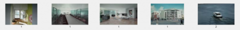
Multimedia tools and applications are growing exponentially with the advent of the Information and Communication Tools (ICT). In the current scenario, with the available sophisticated digital imaging techniques and powerful software for generating Computer Graphics (CG) images are highly challenging to classify the real images with human visual system. Figure 1 shows a set of images with both Photographic (PG) and CG. Top four images represent CG and bottom four represents PG images. PG images are usually taken using digital cameras and CG images are spoofing images created by software based on the real images. CG images has wide application in areas like virtual reality, video games, animations, educational simulations, film industry and many others [1]. There are large numbers of software available for generating CG images which are sometimes used illegally. Effectively differentiating PG and CG images are highly required in criminal investigations, fake news identification, newspaper images, identifying the originality of images in case of defaming to person of social importance based on image. The misuse of CG imaging has created an alarming need to image forensics experts [2] and other software based techniques.
Recently, many researchers have proposed interesting techniques to classify PG and CG images. Commonly used approach to solve this problem is to preprocess the image followed by feature extraction and use any classification method. Mostly for preprocessing, conversions techniques such as RGB to grayscale [3-5] or any band pass filters [6] are used. Existing work can be grouped as hand crafted and Convolutional Neural Network (CNN)-based feature extractors [6].
Figure 1. Examples of CG and PG images taken from dataset, top row: CG images; bottom row: PG images
Handcrafted feature extraction techniques are implemented using well known methods such as Discrete Wavelet Transform (DWT) [7], Discrete Fourier Transform (DFT) [8], Quaternion Wavelet Transform (QWT) [9], Local Binary Pattern (LBP) [10], Content-Based Image Retrieval (CBIR), Composite Visual features and many others. Even-though the handcrafted feature extractor performs well and provides better accuracy, it cannot be generalized [11]. In other words, it is designed for a particular application and dataset. It focuses only on the selected features of the images. Moreover these techniques rely on the human supervision and expert knowledge to choose the features which results in limited accuracy for complex and large datasets. To overcome the pitfalls in the handcrafted feature extractor, CNN based techniques can be used. CNN based feature extractor provides more accurate results due to its diverse nature of learning the holistic feature from an image [9].
CNN based methods are widely used to study the features and visual contents of the images. Well known CNN architecture includes AlexNet [12], GoogleNet [13] and after the evolution of Deep CNN VGGNet [14], DenseNet [15] and other techniques are also used. Many works have proposed CNN based models to solve this problem. Recently, many deep learning based methods are proposed using different models and methods like attention based dual branch CNN [16], deep learning model with transfer learning [17], and a self-coding module to differentiate image based on color correlation [18] were implemented for feature extraction.
The CG and PG images visually look very similar and cannot be easily differentiated using human visual system. The image formation process of the PG and CG images are entirely different, which leads to different inherent properties for these images. Based on the literature, the image classification based on feature extractor for PG and CG images can be broadly classified as hand crafted and CNN based feature extraction methods. Most of the work focuses on classification using inherent properties of the images.
Hand crafted feature extractor utilizes various features such as color, brightness, edges, texture and many others. Apart from these features, wavelet transforms are used to study characteristics like mean, variance, and skewness [7]. Geometry based feature selection on textural characteristics is proposed and an accuracy of 83% was obtained. Image wavelet transform, discrete wavelet transform, discrete cosine transform-based techniques were also used for handcrafted feature selection [19]. Color histogram, edges, moments and texture interpolation based techniques were also used [20]. In another work, transform domain based wavelet methods are fused with noise statistic feature selection for image classification [7]. Even, first order and second order differential signals also used for feature selection. On the other hand, hand crafted feature selection were also used with Support Vector Machine classifiers [21]. Homo-morphic filtering and SVM classifier were used to classify the PG and CG images [22]. Wang et al. proposed quaternion wavelet transform domain for choosing the color based feature extracted using RGB images [23]. Even though handcrafted feature extractor has shown better performance, it has few limitations including (1) Not suitable for large dataset with more samples (2) Accuracy may reduce on smaller datasets (3) Large number of features are required for hand crafted feature extractor which leads to larger processing time.
To overcome the limitations with hand crafted feature extractor, deep learning and CNN based methods are used, which shows better performance by automatically learning important features of the images. There are many works demonstrating CNN to classify CG and PG images [8, 24]. Few works have also reported the transfer learning model for image classification [25]. TL based methods has the advantage of learning from the previous task to solve the new task with similar problem. A dual path CNN network is also used and output were combined and fed to the Recurrent Neural Network (RNN) [26]. Even though there are many advantages of using CNN instead of hand crafted feature selection, there are many new techniques are being proposed to improve the accuracy of the CNN based image classification.
The main contributions of this work:
This section describes the framework used to extract the deep features using transfer learning (TL) model namely SqueezeNet. Moreover, this work also analyses the performance of other networks like Googlenet, VGG18, Alexnet and ResNet50. These pre-trained models were trained using popular image dataset namely ImageNet. It comprises more than 1.3 million images from distinct classes. The deep features obtained through transfer learning are classified based on the knowledge of softmax layer. The generic framework is shown in Figure 2.
Figure 2. Framework for transfer learning
3.1 Transfer learning
Transfer learning is a useful technique to work with smaller dataset and resource. It is a method of knowledge transfer to a new task through learned weights of the related task. Based on the literature, methods of knowledge transfer can be broadly grouped into four:
Transfer learning process uses pre-trained deep models, instead of developing a new deep architecture. Most of the TL models have shown better performance over diverse application domains. The main advantage of using TL models is reduction of training data and time. TL can be used in either of the two folds: i) feature extractor followed by a new classifier ii) parameter tuning framework along with available modules. The significance of transfer learning relies on enhancing the learning task to prune the conditional probability $P\left(\frac{y^t}{x^t}\right)$. Transfer learning updates the knowledge on new domain ‘Dt’ using the learned weights on trained/source domain ‘Ds’. Squeezenet, Googlenet, VGG18, Alexnet, ResNet50 are the best examples of TL based models. The details of these models are enlisted in Table 1.
Table 1. Details of the transfer models
|
S. No |
Transfer Models |
# layers |
#Connections |
|
1 |
Squeezenet |
68 |
75 |
|
2 |
Googlenet |
144 |
170 |
|
3 |
VGG18 |
47 |
46 |
|
4 |
Alexnet |
25 |
24 |
|
5 |
ResNet50 |
177 |
192 |
Steps involved in transfer learning are as follows:
Step1: Preprocess the dataset images
Step2: Modify the pre-trained layers and making it suitable for our problem. The learned SqueezeNet weights are transferred to the computer graphic image identification task. The output layer or classification layer is modified in accordance with the binary classification task.
Step3: Derive the transfer features from the pre-trained models
Step4: Choose the best model, save it and use it to classify the images
3.2 Deep feature extraction using pre-trained CNN models
3.2.1 AlexNet [12]
The popularly known pre-trained model called AlexNet consists of eight layers. Among these, the first five layers do convolution process and remaining three layers are fully connected. As the network is trained for 1000 labels the output of the fully connected layer is followed by a 1000 way softmax layer. The useful techniques like ReLu and dropout are used in AlexNet. The input size of the network is 227X227.Initialization of model parameters is the key factor to be considered for training the AlexNet.
3.2.2 GoogleNet [13]
GoogleNet proposed by google research, consists of 22 layers and has shown improved performance over AlexNet. It differs from other architectures because it uses different kinds of modules namely 1X1 convolution, global average pooling and inception. The 1X1 convolution layer reduces the parameters which in turn increases the depth of the network. Instead of using fully convoluted Layer as AlexNet, it uses global average pooling for maintaining the trade-off between accuracy and number of parameters. In the inception module, convolution and max pooling are done parallel for both input and output.
3.2.3 VGG-18 [14]
VGG net was developed by Simonyan and Zisserman. It is a uniform architecture with 16 convolution layers. It consists of more filters and few 3X3 convolutions. It is the commonly used pre-trained models to extract the deep image features. The available weights of the VGG network are used as a baseline feature descriptor. Any how the huge parameters make it difficult to handle. One convolution layer and ReLu activation function is removed from VGG19 to get VGG18 network.
3.2.4 ResNet50 [27]
ResNet50 is the successor of ResNet152 which consists of 152 layers. ResNet50 is one of the pre-trained models with 50 deep layers trained on more than one million images. Each block in the ResNet is two or three layers deep. Size of the input and first layer is 224 X 224 and 7 X7 respectively. The bottle neck layer follows the convolution windows of size 1X1, 3X3, 1X1.
3.2.5 SqueezeNet [28]
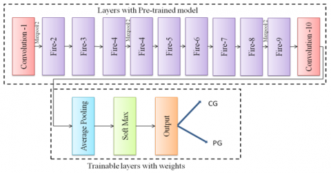
SqueezeNet is tiny neural network architecture with optimized parameter adaptable for small memory and can be transmitted over network efficiently. SqueezeNet is an 18 layer deep CNN designed to provide high degree of accuracy with minimum number of neural network layers. It consists of convolutional layer, max pooling layer, average pooling layer, fire layer and one output softmax layer. It achieves better accuracy then other Deep CNN architecture with fewer layers. SqueezeNet has a convolutional layer followed by eight fire layers and one convolutional layer at the end. Number of filters used in fire module is increased and after final convolutional layer max pooling will be performed by the SqueezeNet architecture. Figure 3 and Table 2 shows the squeezeNet architecture in detail.
Figure 3. SqueezeNet model
Table 2. Layer configuration of feature extractor
|
Layer |
Type |
Output Size |
|
Input |
- |
227 X 227 X 3 |
|
Conv 1 |
(Conv + ReLu) |
113 X 113 X 64 |
|
Pool 1 |
Max Pool |
56 X 56 X 64 |
|
Fire 2 |
(Squeeze + ReLu-Expand + ReLu-Concat) |
56 X 56 X 16 |
|
|
(Expand + Relu)/2 |
56 X 56 X 64 |
|
|
|
56 X 56 X 128 |
|
Fire 3 |
(Squeeze + ReLu-Expand + ReLu-Concat) |
56 X 56 X 16 |
|
|
(Expand + Relu)/2 |
56 X 56 X 64 |
|
|
|
56 X 56 X 128 |
|
Pool 3 |
Max Pool |
28 X 28 X 128 |
|
Fire 4 |
(Squeeze + ReLu-Expand + ReLu-Concat) |
28 X 28 X 32 |
|
|
(Expand + Relu)/2 |
28 X 28 X 128 |
|
|
|
28 X 28 X 256 |
|
Fire 5 |
(Squeeze + ReLu-Expand + ReLu-Concat) |
28 X 28 X 32 |
|
|
(Expand + Relu)/2 |
56 X 56 X 128 |
|
|
|
56 X 56 X 256 |
|
Pool 5 |
Max Pool |
14 X 14 X 256 |
|
Fire 6 |
(Squeeze + ReLu-Expand + ReLu-Concat) |
14 X 14 X 48 |
|
|
(Expand + Relu)/2 |
14 X 14 X 192 |
|
|
|
14 X 14 X 384 |
|
Fire 7 |
(Squeeze + ReLu-Expand + ReLu-Concat) |
14 X 14 X 48 |
|
|
(Expand + Relu)/2 |
14 X 14 X 192 |
|
|
|
14 X 14 X 384 |
|
Fire 8 |
(Squeeze + ReLu-Expand + ReLu-Concat) |
14 X 14 X 64 |
|
|
(Expand + Relu)/2 |
14 X 14 X 256 |
|
|
|
14 X 14 X 512 |
|
Fire 9 |
(Squeeze + ReLu-Expand + ReLu-Concat) |
14 X 14 X 64 |
|
|
(Expand + Relu)/2 |
14 X 14 X 256 |
|
|
|
14 X 14 X 512 |
|
Conv 10 |
(Conv + ReLu) |
14 x 14 X 2 |
|
Pool 10 |
Global average pool |
1 X 1 X 2 |
|
Output |
Softmax |
1 X 1 X 2 |
As described in section 3, this work aims to select the best pre-trained model which is suitable for distinguishing CG images from PG images. To demonstrate the performance of the pre-trained models, 1000 CG and 1000 PG images are chosen from photo realistic [29] and Colombia University Dataset [30] respectively. All these images are RGB in nature. Further the details about the dataset are detailed in Table 3. The defined problem aims to classify the images into two viz, computer graphic and photographic images. The labels are {C1, C2} respectively. The cross entropy loss function is used to define the conditional probability distribution. It is given as,
$H(p, q)=-\sum_{x \in X} p(x) \log q(x)$ (1)
where, $p(x)=\left\{\begin{array}{l}1, \text { if } x \in C_1 \\ 0 . \text { if } x \in C_2\end{array}\right.$.
The effectiveness of the pre-trained models is analyzed using the evaluation metric called classification accuracy. The accuracy can be mathematically expressed as,
$A=\frac{T N+T P}{T N+F N+T P+F P}$ (2)
where, TP denotes the count of CG images classified as CG by TL, TN provides the number of PG images classified as PG by TL, FP represents the count of PG images classified as CG by TL, and FN gives the number of CG images classified as PG images by TL. The classification accuracy is verified in different ways by varying the folding ratio (training: validation) ratio as 70:30 and 80:20. Sample images chosen for training and validation of the TL models are shown in Figure 4. Also, the pre-trained models are evaluated using images with and without data augmentation. In this work data augmentation is carried out using image Data Agumenter object of MATLAB and different methods are used for augmentation such as rotation, horizontal and vertical scaling and translation. The training set contains the augmented data whereas the test set has only real images. The performance of the model was better using augmentation due to the large training data set compared to without augmentation. It is mandatory to evaluate the TL models under same baselines. Hence, the parameters of the TL models are set as.
Table 3. Dataset details
|
Class |
Category |
Characteristics |
|
1 |
PG |
House, living area, natural scenery, Human, fruits, flowers, animals, birds, car, buildings |
|
2 |
CG |
House, living room, insects, animals, birds, human, flowers, metals, car, sea, table, sculpture |
Follows: #Epochs=10, initial learning rate=0.001, validation frequency=5.TL is chosen in this work to reduce the time involved in developing a new architecture and training the images.
Table 4. Comparison of validation accuracy
|
Models |
80:20 ratio |
70:30 ratio |
||
|
No augmentation |
With augmentation |
No augmentation |
With augmentation |
|
|
SqueezeNet |
90.42 |
93.75 |
89.58 |
91.25 |
|
GoogleNet |
88.75 |
90.625 |
88.33 |
90.42 |
|
AlexNet |
87.5 |
88.75 |
87.50 |
90.42 |
|
Resnet50 |
86.25 |
86.25 |
85.42 |
85.42 |
|
VGG18 |
83.125 |
84.375 |
83.33 |
86.25 |
Table 5. Testing accuracy for SqueezeNet
|
Models |
80:20 ratio |
70:30 ratio |
||
|
No augmentation |
With augmentation |
No augmentation |
With augmentation |
|
|
SqueezeNet |
90 |
93 |
89 |
91.25 |
(a) Samples of training images for TL
(b) Samples of validation images for TL
Figure 4. Sample images
(a) Folding ratio 70:30
(b) Folding ratio 80:20
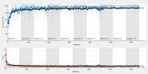
Figure 5. Variation of accuracy and loss with number of epochs for Squeeze Net model
The deep features for discriminating CG and PG images are extracted from the TL models like ResNet50, VGG16, AlexNet, GoogleNet and SqueezeNet available in MATLAB2021. The weights of these models were trained on huge dataset for large number of classes. The input layer, fully connected layer and the classification layer are fine tuned in predicting the class for the defined problem. Table 4 enumerates the performance of different pre-trained models and it is observed that SqueezeNet model is much suitable for classifying CG images from PG images preferably for small scale dataset. The experimental results were reported based on four variation viz. with augmentation in input data, without augmentation in input data, folding ratio-70:30, 80:20. It is evident from Table 4 that CG/PC classification is working satisfactorily for the folding ratio 80:20 and achieved a good validation accuracy of 93.75% on SqueezeNet for augmented data. It is surprising to that ResNet50 doesn’t show any variation for augmentation in both folding ratio.
After observing the performance of the SqueezeNet model, testing is performed on this model. The effectiveness of SqueezeNet is enumerated in Table 5. Table 5 reports that SqueezeNet model is working best when the data is augmented and the folding ratio is 80:20. Figure 5 shows the variation of accuracy and loss with number of epochs for SqueezeNet model for different folding ratio.
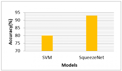
As we are working on a small-scale dataset, it is also essential to compare the SqueezeNet model with machine learning classifier. The handcrafted feature used is independent component analysis which provides the sparse representation and the extracted feature is classified using support vector machine (SVM). Comparison of performance using SVM and SqueezeNet is shown in Figure 6.
Figure 6. SVM Vs SqueezeNet
This paper has analyzed a method to distinguish CG and PG images using SqueezeNet model, which is not explored in the literature. Initially, the input layer, fully convoluted layer and classification layer of all the chosen pertained models were modified according to the desired problem. The best transfer learning approach was chosen by comparing validation accuracy among all pre-trained models. Later, it was evident that SqueezeNet outperforms other models with a validation accuracy of 93.75% and it was selected for testing the transfer learning approach in classification. A testing accuracy of 93% was achieved by SqueezeNet with minimal training time and resource.
[1] Suwajanakorn, S., Seitz, S.M., Kemelmacher-Shlizerman, I. (2017). Synthesizing Obama: Learning lip sync from audio. ACM Transactions on Graphics (ToG), 36(4): 1-13. https://doi.org/10.1145/3072959.3073640
[2] Ansari, M.D., Ghrera, S.P., Tyagi, V. (2014). Pixel-based image forgery detection: A review. IETE Journal of Education, 55(1): 40-46. https://doi.org/10.1080/09747338.2014.921415
[3] Meena, K.B., Tyagi, V. (2019). A copy-move image forgery detection technique based on Gaussian-Hermite moments. Multimedia Tools and Applications, 78(23): 33505-33526. https://doi.org/10.1007/s11042-019-08082-2
[4] Meena, K.B., Tyagi, V. (2019). Methods to distinguish photorealistic computer generated images from photographic images: A review. In International Conference on Advances in Computing and Data Sciences, pp. 64-82. https://doi.org/10.1007/978-981-13-9939-8_7
[5] Tokuda, E., Pedrini, H., Rocha, A. (2013). Computer generated images vs. digital photographs: A synergetic feature and classifier combination approach. Journal of Visual Communication and Image Representation, 24(8): 1276-1292. https://doi.org/10.1016/j.jvcir.2013.08.009
[6] Ni, X., Chen, L., Yuan, L., Wu, G., Yao, Y. (2019). An evaluation of deep learning-based computer generated image detection approaches. IEEE Access, 7: 130830-130840. https://doi.org/10.1109/ACCESS.2019.2940383
[7] Lyu, S., Farid, H. (2005). How realistic is photorealistic? IEEE Transactions on Signal Processing, 53(2): 845-850. https://doi.org/10.1109/TSP.2004.839896
[8] Meena, K.B., Tyagi, V. (2021). Distinguishing computer-generated images from photographic images using two-stream convolutional neural network. Applied Soft Computing, 100: 107025. https://doi.org/10.1016/j.asoc.2020.107025
[9] Wang, J., Li, T., Luo, X., Shi, Y.Q., Jha, S.K. (2018). Identifying computer generated images based on quaternion central moments in color quaternion wavelet domain. IEEE Transactions on Circuits and Systems for Video Technology, 29(9): 2775-2785. https://doi.org/10.1109/TCSVT.2018.2867786
[10] Li, Z., Zhang, Z., Shi, Y. (2014). Distinguishing computer graphics from photographic images using a multiresolution approach based on local binary patterns. Security and Communication Networks, 7(11): 2153-2159. https://doi.org/10.1002/sec.929
[11] Zhang, R.S., Quan, W.Z., Fan, L.B., Hu, L.M., Yan, D.M. (2020). Distinguishing computer-generated images from natural images using channel and pixel correlation. Journal of Computer Science and Technology, 35(3): 592-602. https://doi.org/10.1007/s11390-020-0216-9
[12] Krizhevsky, A., Sutskever, I., Hinton, G.E. (2012). Imagenet classification with deep convolutional neural networks. Advances in Neural Information Processing Systems, 25.
[13] Szegedy, C., Liu, W., Jia, Y., et al. (2015). Going deeper with convolutions. In Proceedings of the IEEE Conference on Computer Vision and Pattern Recognition, pp. 1-9. https://doi.org/10.1109/CVPR.2015.7298594
[14] Simonyan, K., Zisserman, A. (2014). Very deep convolutional networks for large-scale image recognition. arXiv preprint arXiv:1409.1556.
[15] Huang, G., Liu, Z., Van Der Maaten, L., Weinberger, K.Q. (2017). Densely connected convolutional networks. In Proceedings of the IEEE Conference on Computer Vision and Pattern Recognition, pp. 4700-4708. https://doi.org/10.1109/CVPR.2017.243
[16] He, P., Li, H., Wang, H., Zhang, R. (2020). Detection of computer graphics using attention-based dual-branch convolutional neural network from fused color components. Sensors, 20(17): 4743. https://doi.org/10.3390/s20174743
[17] Hussain, M., Bird, J.J., Faria, D.R. (2018). A study on CNN transfer learning for image classification. In UK Workshop on Computational Intelligence, pp. 191-202. https://doi.org/10.1007/978-3-319-97982-3_16
[18] Ren, S., He, K., Girshick, R., Sun, J. (2017). Faster R-CNN: Towards real-time object detection with region proposal networks. IEEE Transactions on Pattern Analysis and Machine Intelligence, 39(6): 1137-1149. https://doi.org/10.1109/TPAMI.2016.2577031
[19] Chen, W., Shi, Y.Q., Xuan, G. (2007). Identifying computer graphics using HSV color model and statistical moments of characteristic functions. In 2007 IEEE International Conference on Multimedia and Expo, pp. 1123-1126. https://doi.org/10.1109/icme.2007.4284852
[20] Sankar, G., Zhao, V., Yang, Y.H. (2009). Feature based classification of computer graphics and real images. In 2009 IEEE International Conference on Acoustics, Speech and Signal Processing, pp. 1513-1516. https://doi.org/10.1109/ICASSP.2009.4959883
[21] Xu, B., Wang, J., Liu, G., Dai, Y. (2011). Photorealistic computer graphics forensics based on leading digit law. Journal of Electronics (China), 28(1): 95-100. https://doi.org/10.1007/s11767-011-0474-3
[22] Wang, X., Liu, Y., Xu, B., Li, L., Xue, J. (2014). A statistical feature based approach to distinguish PRCG from photographs. Computer Vision and Image Understanding, 128: 84-93. https://doi.org/10.1016/j.cviu.2014.07.007
[23] Wang, J., Li, T., Shi, Y.Q., Lian, S., Ye, J. (2017). Forensics feature analysis in quaternion wavelet domain for distinguishing photographic images and computer graphics. Multimedia tools and Applications, 76(22): 23721-23737. https://doi.org/10.1007/s11042-016-4153-0
[24] Cui, Q., McIntosh, S., Sun, H. (2018). Identifying materials of photographic images and photorealistic computer generated graphics based on deep CNNs. Comput. Mater. Continua, 55(2): 229-241. https://doi.org/10.3970/cmc.2018.01693
[25] Nguyen, H.H., Tieu, T.N.D., Nguyen-Son, H.Q., Nozick, V., Yamagishi, J., Echizen, I. (2018). Modular convolutional neural network for discriminating between computer-generated images and photographic images. In Proceedings of the 13th International Conference on Availability, Reliability and Security, pp. 1-10. https://doi.org/10.1145/3230833.3230863
[26] He, M. (2019). Distinguish computer generated and digital images: A CNN solution. Concurrency and Computation: Practice and Experience, 31(12): e4788. https://doi.org/10.1002/cpe.4788
[27] He, K., Zhang, X., Ren, S., Sun, J. (2016). Deep residual learning for image recognition. In Proceedings of the IEEE Conference on Computer Vision and Pattern Recognition, pp. 770-778. https://doi.org/10.1109/CVPR.2016.90
[28] Ucar, F., Korkmaz, D. (2020). COVIDiagnosis-Net: Deep Bayes-SqueezeNet based diagnosis of the coronavirus disease 2019 (COVID-19) from X-ray images. Medical Hypotheses, 140: 109761. https://doi.org/10.1016/j.mehy.2020.109761
[29] Photographic computer graphic image database. www.%0Airtc.org, accessed on 12 June 2022.
[30] Ng, T.T., Chang, S.F., Hsu, J., Pepeljugoski, M. (2005). Columbia photographic images and photorealistic computer graphics dataset. Columbia University, ADVENT Technical Report, pp. 205-2004.