An Approach for Enhancement of MR Images of Brain Tumor

A brain tumor is a cell growth that is uncontrolled in any brain area [1]. A total of 400000 cases of brain tumors are diagnosed globally every year, of which 120000 patients become cancerous due to late diagnosis [2]. As per the GLOBOCAN 2020 report, 308102 new cancerous brain tumor (1.6% of total cancerous tumor) cases were added in 2020, and 251329 lost their life (2.5% overall mortality rate due to cancerous tumor) worldwide [3]. According to the central nervous system of India, around 0.005% to 0.01% of the population is diagnosed with brain tumors, of which 2% have cancerous brain tumors [4]. According to the American Brain Tumor Association and the World Health Organization (WHO), the brain tumor grading system employs a range from one to four grades for designating tumors as malignant or non-cancerous [5]. According to this scale, grades I and II fall under non-cancerous (Benign) tumors and are slow growth rate tumors. Therefore, patients with grade II tumors need proper monitoring and regular observation to cure well on time before these become grade III or malignant. Grades III and IV are categorized as malignant tumors and are high-grade tumors with high growth rates [6]. The above grading plays an essential role in the survival of brain tumor patients that depends on the accurate detection of brain tumors. Medical imaging techniques are adopted these days to diagnose brain tumors. Non-invasive diagnosis methods in medical imaging [7], Computed Tomography (CT) [8], and Magnetic Resonance Imaging (MRI) are widely used in the present scenario. MRI gives more valuable information than CT for brain tumor detection and provides a tumor progress model during treatment [9]. MRI techniques of image modalities of brain tumors help experts with early diagnosis and treatment. The MR images may contain some noise, and this may affect the accurate diagnosis of brain tumors. Thus it requires enhancing the image quality to increase the detection accuracy of brain tumors.

In this paper, an approach for enhancing the MR images is proposed. The Comprehensive Learning-based Elephant Herding Optimization technique has been proposed to optimize the smoothness factor of Bi-Histogram Equalization with Adaptive Sigmoid Function (BEASF), which gives better results in terms of visual inspection as well as parametric evaluation metrics. The enhanced images show better feature variance without distracting the structural similarity index metrics of brain tumor MR images.

The rest of the paper is organized as follows. The existing work in the field of MR image enhancement is presented in Section 2. the material and proposed methodology are described in Section 3. Section 4 contains information regarding the database used. The output findings and the Friedman rank test is presented in Section 5 to examine the ranking of the proposed methodology. Finally, Section 6 summaries the proposed approach and its future scope.

An approach for enhancing MR images has been described in this paper. Compared to other techniques, the output of Bi-Histogram Equalization with Adaptive Sigmoid Function (BEASF) is superior without sacrificing image information [38]. But the problem with BEASF is the selection of an optimal value of the smoothening factor. So an improved metaheuristic technique is required for this purpose. A comprehensive learning strategy is employed to improve the performance of EHO, and this improved EHO is used for optimizing the value of smoothening factor in the BEASF.

3.1 Bi-Histogram equalization with adaptive sigmoid function

B EASF gives more visual quality than original images and ignores brightness preservation. Its qualitative parameters indicate that it preserves brightness [39]. BEASF, contains three steps i.e. histogram splitting, creation of sigmoid function, and mapping [40].

3.1.1 Histogram splitting

The original image (I₁) with the size M×N has the possible intensity levels (£). The mean intensity of the image is:

Mean Intensity $(m)=\frac{\sum_{i=0}^{M-1} \sum_{j=0}^{N-1} I_1(i, j)}{M \times N}$           (1)

Using the mean intensity as a splitting point, the original image histogram H is separated into two sub-histograms, H₁ and H₂, $H=H_1 \cup H_2$, where $H_1=\left\{h_0, h_1, \ldots h_m\right\}$ and $H_2=\left\{h_{m+1}, h_{m+2}, \ldots h_{£-1}\right\}$.

The value of the probability density function of two sub histograms is evaluated after splitting. The probability density function is:

$p_1(k)=\frac{H_1(k)}{\sum_{n=0}^m \quad H_1(n)}$           (2)

$p_2(k)=\frac{H_2(k)}{\sum_{n=m+1}^{£-1} \quad H_2(n)}$          (3)

where, $k \in\{0,1,2 \ldots £-1\}$ is an intensity level.

The cumulative distribution functions for H₁ and H₂ are:

$c_1(k)=\sum_{n=0}^k p_1(n)$           (4)

$c_2(k)=\sum_{n=m+1}^k \quad p_2(n)$           (5)

Then µ₁ and µ₂ are the medians of sub histogram H₁ and H₂ can be found when the following conditions are satisfied.

$c_1\left(\mu_1\right)=0.5$ and $c_2\left(\mu_2\right)=0.5$.

3.1.2 Sigmoid function creation

In this process, two parametric nonlinear sigmoid functions (Eq. (8) and (9)) are created by taking the origins of the sigmoid functions at the medians defined in sub-histograms. The value of k is normalized using the following Eq. (6) and (7):

$z_1(k)=\frac{5\left(k-\mu_1\right)}{m}, k \leq m$          (6)

$z_2(k)=\frac{5\left(k-\mu_2\right)}{£-1-m}, k>m$          (7)

Here ‘z₁(k)’ and ‘z₁(k)’ are the input values used for the calculation of the sigmoid function, ‘k’ is the intensity level, ‘m’ is the mean intensity, µ₁ and µ₂ are the medians of sub-histogram H₁ and H₂, £ is the possible intensity levels.

$s_1(k)=\frac{1}{1+e^{-\gamma z_1(k)}}, k \leq m$          (8)

$s_2(k)=\frac{1}{1+e^{-\gamma z_2(k)}}, k>m$           (9)

Here, s₁(k) and s₂(k) are non-linear parametric sigmoid functions, ‘k’ is the intensity level, and γ is the smoothness factor.

After the normalization of the sub histogram, it will fit the desired boundaries of the sigmoid function, $z_1(k), z_2(k) \in[-5,5]$, the convenient range for sigmoid function, the values of smoothening factor across this range will be either 0 or 1.

For the above sigmoid function, the range will be [0, m] and [m, £-1]. The smoothness factor of the sigmoid function is γ. A smoother sigmoid function is created by a lower value of γ, which affects the value of contrast in the enhanced image.

3.1.3 Mapping

The sigmoid function calculated in the previous steps is utilized for finding the values of histogram equalization and stretching. The formulation of the histogram equalization is as follows:

$u_1(k)=L_0+\left(m-L_0\right) s_1(k)$          (10)

$u_2(k)=m+\left(L_1-m\right) s_2(k)$          (11)

L₁ and L₀ are the desirable upper and lower limit of the dynamic range in enhanced images, here L₀=0 and L₁=£-1. After mapping, the histogram stretching has been performed by using the equation below:

$S T F=\left\{\begin{array}{l}L_0+\alpha_1\left(u_1(k)-\min \left(u_1\right)\right) \text { when } k \leq m \\ m+\alpha_2\left(u_2(k)-\min \left(u_2\right)\right) \text { when } k>m\end{array}\right.$          (12)

where, $\alpha_1=\frac{m-L_0}{\max \left(u_1\right)-\min \left(u_1\right)}$ and $\alpha_2=\frac{L_1-m}{\max \left(u_2\right)-\min \left(u_2\right)} \quad$.

The mappings calculated in this step are applied to every pixel of the input image for image enhancement.

3.2 Elephant herding optimization

The EHO method was introduced by Wang et al. [41]. The process of EHO depends on the herding behavior of elephants. After growing up, the male elephants leave their families to form their self-groups. The elephants are divided into distinct clans and live together under the direction of a matriarch. The two behaviors described above are represented using two operators. The clan updating operator and the separation operator are idealized to construct a simple global optimization approach.

3.2.1 Clan updating operator

When the elephants are moving surrounding the matriarch, the positions of individual elephants in the clan are marked by the matriarch after every movement of individuals. Then the newest position of the elephant is considered as:

$E_{n e w, Q_n, k}=E_{Q_n, k}+\delta \times\left(E_{\text {best }, Q_n, k}-E_{Q_n, k}\right) \times t$          (13)

where, $E_{n e w, Q_n, k}$ is the elephant’s latest position in the clan. $E_{Q_n, k}$ is the $k^{t h}$ elephant’s old position in the clan $Q_n$. $E_{\text {best }, Q_n}$ is the fittest elephant in clan $Q_n$, $t \in[0,1]$, is a uniformly distributed random number. $\delta \in[0,1]$ is a factor by which $E_{Q_n, k}$ affected by matriarch $Q_n$. It is also known as the scaling factor. The fittest elephants in the clan are represented as:

$E_{\text {new}, Q_n, k}=\gamma \times E_{\text {centre}, Q_n}$           (14)

$E_{n e w, Q_n, k}$ is getting the data of all elephants present in the clan. $\gamma \in[0,1]$, factor by which influence of $E_{\text {centre }, Q_n}$ on $E_{n e w, Q_n, k}$ is determined. $E_{\text {centre }, Q_n, d}$ is the center of the clan $Q_n$ for the $d^{t h}$ dimension and can be obtained by the following equation:

$E_{\text {centre }, Q_n, d}=\frac{1}{\theta_{Q_n}} \times \sum_{k=1}^{\theta_{Q_n}} E_{Q_n, k, d}$          (15)

where, 1 ≤ d ≤ D shows the $d^{t h}$ dimension in which D is the total dimension.

3.2.2 Separating operator

When male elephants complete their grown-up stage in the clan, they leave the family group. Enhancement of EHO algorithm searching capability within a condition when for every generation, the separating operator is completed by all individual elephants with worst fitness is described as follows:

$E_{\text {worst }, Q_n}=E_{\min }+\left(E_{\max }-E_{\min }+1\right) \times$ rand           (16)

where, $E_{\text {worst}}, Q_n$ is, the worst's elephant in the clan, rand represents the stochastic and uniform distribution having range between [0, 1]. E_max and E_min are the individual elephant's upper and lower bound positions.

3.3 Comprehensive learning-based EHO (CLEHO)

The standard EHO has some drawbacks. Due to the updating operator, the exploration is influenced by unreasonable convergence towards the origin and unbalanced exploration [42]. The clan-updating operator may only update clans inside its own [43]. Therefore, comprehensive learning [44] is introduced in this work to improve the drawbacks of standard EHO. In comprehensive learning, three different learning strategies have been introduced to update the positions of elephants that are described below:

3.3.1 Learning strategy I

For improving the exploration of the algorithm, Eq. (17) is used, and it gives better results. It depends on the worst and best clan individuals of the current clan to enhance the searchability of EHO.

$E_{n e w, Q_n, k}=E_{Q_n, k}+\left(\varphi_1 \times E_{\text {best }, Q_n, k}-\left|E_{Q_n, k}\right|\right)-\varphi_2\left(E_{\text {worst }, Q_n, k}-\left|E_{Q_n, k}\right|\right)$,

if $0 \leq T_{\text {switch }} \leq 1 / 3$          (17)

φ₁ and φ₂ are the two random numbers, and T_switch is switch probability and distributed uniformly between 0 to 1.

3.3.2 Learning strategy II

In this strategy, the mean and best clan individuals are used to update the positions of the current clan individual. It is expressed as:

$E_{\text {new, } Q_{n,}, k}=E_{Q_{n, k}}+\left(\varphi_3 \times E_{\text {best }, Q_{n,}k}-\left|E_{Q_{n, k}}\right|\right)-\varphi_4\left(\bar{X}-\left|E_{Q_{n, k}}\right|\right)$,

if $\frac{1}{3}<T_{\text {switch }} \leq 2 / 3$          (18)

where, $\bar{X}$ is the mean position of the clan. φ₃ and φ₄ are the two random numbers subjected to normal distribution.

3.3.3 Learning strategy III

This strategy utilizes the position of the worst clan individual and two randomly selected clan individuals to update the position of the current clan individual. This strategy is mathematically modeled as:

$E_{\text {new, } Q_n, k}=E_{Q_n, k}+\left(\varphi_5 \times E_{\text {best }, Q_n, k}-E_{Q_n, k}\right)-\varphi_6\left(E_p-E_q\right)$,

if $\frac{2}{3}<T_{\text {switch }} \leq 1$          (19)

where, p and q are two integer ranges between one to $\theta_{Q_n}$ and not equal to each other, at any instance. φ₅ and φ₆ are the two random numbers between zero and one.

3.4 Proposed methodology

In the proposed work, a Comprehensive Learning-based Elephant Herding Optimization (CLEHO) is proposed to enhance MR images of brain tumors, taking 1577 images from the Figshare [45] data set publicly available. The proposed CLEHO algorithm is used for optimizing the value of the smoothness factor (γ) of the sigmoid function of BEASF. The proposed CLEHO optimizes the smoothness factor by initiating random solutions and further improves them by selecting a learning strategy based on the switching probability (T_switch). In this manner, CLEHO gives the best value for the smoothness factor.

1.jpg

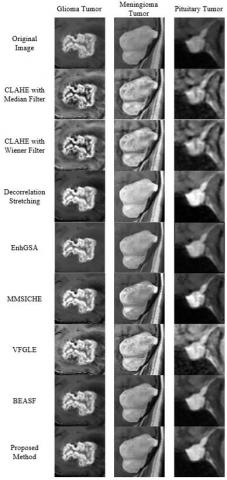
Figure 1. Visual analysis of original and enhanced images

A methodology using Comprehensive Learning-based Elephant Herding Optimization (CLEHO) is employed to optimize the smoothing factor of BEASF, which is used to enhance the image quality of MR images. For the proposed CLEHO-based approach, the population is 50, and 500 iterations are taken to optimize the value of the smoothness factor (γ) of the Bi-Histogram equalization with adaptive sigmoid function. The experimental results are performed on an Intel I3 7^th generation processor system using Windows 10 Pro operating system having 8 GB RAM. The proposed methodology has been implemented in MATLAB2021a.

The proposed methodology has processed glioma, meningioma, and pituitary tumor images. The region of suspicion is extracted by cropping the area of interest, and images collected from the Figshare database have been taken for testing. The performance has been evaluated for direct visual inspection and quantitative analysis of glioma, meningioma, and pituitary tumors.

2.jpg

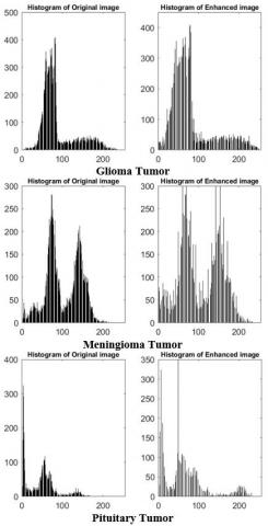
Figure 2. Histogram comparison of original and enhanced images

5.1 Visual inspection

A total of 1577 images are taken for visual inspection in which it has been seen that the region of interest is enhanced. The histograms showing the number of pixels for each tonal value are plotted. It describes the tonal distribution of an image. The proposed method is compared with CLAHE with Median filter [46], CLAHE with Wiener filter [25], Decorrelation [47], Enhancement Gravitational Search Algorithm (EnhGSA) [48], Median Mean based Sub Image Clipped Histogram Equalization (MMSICHE) [49], Variational based Fusion model for Gray Scale image Enhancement (VFGLE) [50], and Bi-Histogram Equalization with Adaptive Sigmoid Function (BEASF) [40]. The visual comparison of the proposed method with other state-of-the-art methods by taking an image from three different type of tumors, shown in Figure 1.

Figure 1 shows that the proposed technique successfully enhances the MR images of all three tumor types. The enhanced images give a better outcome than the other method without losing their originality. A comparison of histograms for the original and enhanced image is shown in Figure 2.

Through visual inspection, it is observed that the contrast and intensity of the enhanced images are stretched only up to that limit where the enhanced images do not lose their visual properties. The enhanced images (Glioma tumor -832, Meningioma tumor- 677, pituitary tumor – 1756) shown have not sacrificed any significant image information.

5.2 Quantitative evaluation

Improving the visual quality of a digital image, often known as image enhancement, is a subjective process. The identification of one method that provides a better quality image may vary from person to person. So, metrics to compare the effects of image enhancement algorithms on image quality are required for proper analysis. Mean Square Error (MSE), Peak Signal to Noise Ratio (PSNR), Mean Absolute Error (MAE), Structural Similarity Index Metric (SSIM), Features Similarity Index Metric (FSIM), Riesz transformed based Feature Similarity Index Metric (RFSIM), Spectral Residual base Similarity Index Metric (SRSIM) and Absolute Mean Brightness Error (AMBE) are used for quantitative evaluation of the proposed work. For the quantitative assessment, four images of each type are taken. 901, 796, 1899, and 2300 are of glioma type, while 99, 500, 245, and 281 meningioma type. 1689, 1546, 1332, and 1389 are taken from the pituitary tumor type.

5.2.1 Mean Square Error (MSE)

It is the cumulative squared error between enhanced and original images, and its values are always positive [51]. MSE is calculating the difference between the original and processed images. Mathematically, it is written as:

$M S E=\frac{1}{M \times N} \sum_{i=0}^{M-1} \sum_{j=0}^{N-1}\left(I_2(i, j)-I_1(i, j)\right)^2$           (20)

where, I₂ is the enhanced image of an original image I₁ with dimensions M×N. Table 1 compares the results of MSE when four images of each tumor type are included. It has been observed that the values of MSE for all three types of brain tumors MR images are the lowest for the proposed methodology. In Table 1, the next best MSE value given by BEASF indicates the large performance gap with the proposed method. MMSICHE and EnhGSA are the least performers in Table 1 with regard to the performance of MSE.

5.2.2 Peak signal to noise ratio (PSNR)

5.2.7 Spectral Residual base Similarity Index Metric (SRSIM)

It is based on spectral residual visual saliency mapping approaches. It plays two roles, the first one for characterizing the local quality of an image and the second while assessing the overall quality ratings, demonstrating the relevance of a particular location to the human visual system [60]. SRSIM value range is zero to one. A higher value shows the better quality of the enhanced image. SRSIM between two images is defined as:

$\operatorname{SRSIM}=\frac{\sum_{x \in \Delta} S_L(x) R_m(x)}{\sum_{x \in \Delta} R_m(x)}$          (28)

where, Δ means the entire image special domain, S_L (x) is the similarity, and R_m(x) is the weight importance of $S_L(x)$. SRSIM value is improved in the proposed method and approaches the maximum value that is one. The performance of SRSIM shown in Table 7 strongly recommends the proposed method to enhance brain tumor MR images.

5.2.8 Absolute Mean Brightness Error (AMBE)

It was proposed by Chen et al. in the year 2003 to determine the performance in preserving the originality of an image [61]. It is the difference between the original image and the enhanced image's mean intensity values. It is expressed as:

$A M B E=\mid$ mean intensity of $\left(I_1\right)-$ mean intensity of $\left(I_2\right) \mid$          (29)

The small value of AMBE indicates better enhancement [31]. For the proposed method, values of AMBE are shown in Table 8.

The performance gap with other-state-of-the-art method indicates that better enhancement of brain tumor MR images with the proposed method

The proposed enhancement methodology has been checked on 1577 images in this paper. The results of 12 images (4 of each type) for the evaluation metrics are shown in Tables (1 to 8). An average of each performance evaluation metric has been computed for each tumor type, and the results are indicated in Table 9.

For the proposed method, the minimum value of the MSE average is 0.00002 is much better than BEASF. The worst value is achieved with MMSICHE. The average value of PSNR is around 45, while that of BEASF is 25. MAE is lowest at about 0.004. The average value of SSIM is 0.9877, which is near one means better enhancement. The average value of FSIM is 0.9995, which is higher as compared with other methods. The average value of RFSIM is nearly one (0.9999), and the SRSIM average value is 0.9996. The average value of AMBE is 0.8198 lowest compared with other methods.

5.3 Statistical test

Friedman's mean rank test [62, 63] is used to check the statistical difference between proposed and other state-of-the-art methods. The statistical findings of Friedman's mean rank test for performance evaluation metrics are shown in Table 10. According to the statistical data, the suggested approach is in the first place and surpassed the state-of-the-art methods. The p-value of Friedman's mean rank test is 2.0179×10^-14, which is very low compared to α = 0.05.