Faradila Naim* | Mahfuzah Mustafa | Norizam Sulaiman | Zarith Liyana Zahari
© 2022 IIETA. This article is published by IIETA and is licensed under the CC BY 4.0 license (http://creativecommons.org/licenses/by/4.0/).
OPEN ACCESS
Electromyography (EMG) signals are one of the most studied inputs for driver drowsiness detection systems. As the number of EMG features available can be daunting, finding the most significant and minimal subset features is desirable. Hence, a simplified feature selection method is necessary. This work proposed a dual-layer ranking feature selection algorithm based on statistical formula f EMG signals for driver fatigue detection. In the beginning, in the first layer, 21 filter algorithms were calculated to rank 47 sets of EMG features (25 time-domain and 9 frequency-domain) and applied to six classifiers. Then, in the second layer, all the ranks were re-ranked based on the statistical formula (average, median, mode and variance). The classification performance of all rankings was compared along with the number of features. The highest classification accuracy achieved was 95% for 12 features using the Average Statistical Rank (ASR) and LDA classifier. It is conclusive that a combination of features from the time domain and frequency domain can deliver better performance compared to a single domain feature. Concurrently, the statistical rank ASR performed better than the single filter rank by reducing the number of features. The proposed model can be a benchmark for the enhanced feature selection method for EMG driver fatigue signal.
feature selection, electromyography, driver drowsiness, time-domain features, frequency-domain features, statistical rank
Drowsiness or fatigue is one of the top three causes of road accidents in Malaysia [1]. The use of physiological signals as the input to the driver drowsiness detection systems was widely studied including electromyography (EMG) as a single input sensor [2] or multimodal system [3-5] ]with EMG, electroencephalography (EEG), electrocardiography (ECG) and these inputs are high in performance, reliable, efficient and low cost [6]. In a signal analysis process, the number of signal features can be overwhelming, which may result in a longer processing time. Feature selection is a critical step in signal processing, in which the best minimum set of features with the best performance is selected.
The use of feature selection (FS) methods such as the Fisher filter to rank EEG signals have proven that a single EEG electrode from a wearable EEG device [7] is sufficient to detect driver drowsiness. In a study of steering wheel data for driver fatigue, the features were ranked using Fisher, Pearson, mutual information (MIFS), and T-test filters. Then optimization was done using adaptive neuro-fuzzy inference system (ANFIS) in search of the best subset of features [8]. A hybrid FS method using ReliefF and neighborhood component analysis (NCA) filters achieved 100% classification accuracy using k-nearest neighbor (kNN) for EEG driver fatigue detection [9]. Minimum redundancy, maximum relevancy (MRMR) FS was used in detecting driver fatigue using facial landmarks the eyes and mouth using logic regression model achieves 84% accuracies [10]. Behavioural input is another type of input for driver drowsiness detection systems, which involves machine vision inputs. Video and images of the upper body of the drivers are always used in driver fatigue detection. A study using face image as the input applied with Fisher and principal component analysis (PCA) FS method [11] performs better than the deep neural network (DNN). Sharanabasappa et al. had used ReliefF, Infinite (InFS), Pearson Correlation and Term Variance FS methods to reduce the number of (140 million) features from the driver images to detect drowsiness [12]. Once the best features were selected, the DNN was used for the driver drowsiness system FS in signal processing are; to reduce feature redundancies, improve accuracy, and reduce processing time. Henni et. al in her study, used six types of filters to improve driving fatigue detection using driver’s facial expressions, driving behaviors, and bio-signals. The filters used were: Learning for Local Learning-Based Clustering (LLCFS), Features Selection via Eigenvector Centrality (ECFS), Laplacian, Infinte FS (InFS), and Laplacian score. The proposed model achieved 85% accuracy [13].
Among the EMG advantages are noninvasive, user-friendly, and able to detect muscle fatigue at an early stage [14]. These are the reasons why it is selected as inputs in the driver drowsiness studies. In one of the studies by Aiamklin et al., facial EMG was used to detect light sleep in drivers. An 84% accuracy was achieved by placing the electrodes on the masseter and trapezius muscles [15]. Satti et al. had utilised microneedle electrode EMG on hand-gripping muscles and they found that both the time - domain and frequency-domain features detected the increase in driver drowsiness, which was proportional to the decrease in the handgrip muscle activities [16]. In EMG signal processing, there are more than fifty features in the time and frequency domains [17] that can be studied to reduce drowsiness in drivers [18].
The focus on the FS method for driver drowsiness detection is mostly in the EEG, ECG and vision inputs. There is a lack of studies in feature selection methods for EMG signals in the detection of driver drowsiness. Hence, this paper explores the possibilities of enhanced feature selection methods that will give the best performance in this area. The contributions of this paper are as follows:
The basic framework of the study is shown in Figure 1. The collected data will be pre-processed to remove unwanted noise before performing feature extractions. In the feature extraction step, filtered data will be applied to twenty-five time-domain features equations to acquire the feature values. Meanwhile, for the frequency-domain feature values, the filtered data is first transformed to the frequency domain before applying the nine frequency-domain feature equations. Then, in the first layer FS the features will be ranked using 21 FS filters selected in three groups; time-domain feature group, frequency-domain feature group and combined time and frequency-domain feature group. In the second layer, a new rank based on statistical formula was calculated from the 21 ranks. Then, the features will be classified using all the ranks calculated. The classification performance of all available ranks in first and second layer FS will be compared to select the best subset of features based on the highest classification accuracy and minimum number of features.
2.1 Experimental setup
The data was collected from a driving simulator that was set in the lab. The simulator was comprised of a monitor, a computer with an installed driving game (Need for Speed), a steering wheel with pedal and EMG sensors that would be attached to the biceps brachii on the right arm of the participants. Figure 2 shows the experimental setup of the driving simulator. The participants were required to sleep for seven hours on the night before the experiment and avoid caffeinated drinks within 24 hours before the experiment. A total of 15 participants were recruited (seven males and eight females) with an average age of 23 ± 3 years. All participants filled out the Fatigue Assessment Scale (FAS) [19], which was composed of ten questions to evaluate the participants’ fatigue levels before the driving simulation started. The FAS score was later used to classify the drivers into two classes—fatigue and non-fatigue—in the feature selection and classification stage. Seven out of fifteen samples were labelled fatigue and eight samples were labelled as non-fatigue Personal information such as name, age, driving experience and health were also collected. The experiment was conducted at 2 pm to induce natural drowsiness [4] and the participants drove for two hours on the driving simulator. The collected data in the form of EMG signals were kept as a database for analysis in MATLAB 2020b®. The procedure of this study has been approved with ethics number IREC 2020-070 from International Islamic University Malaysia’s ethics committee.
Figure 1. The research framework of dual-layer ranking feature selection
Figure 2. Experimental setup of the driving simulator
2.2 Signal pre-processing
Approximately three million points were extracted from the Shimmer EMG sensor input. The raw EMG data is first sampled to regenerate the signal in MATLAB. The sampling rate of 512 Hz was chosen in accordance with the hardware requirements of the ShimmerTM EMG sensor. Then, these data were filtered using a Butterworth bandpass filter between 10 and 20 Hz to remove the unnecessary noise. Figure 3 shows an example of the raw and filtered data. The filtered signal, will be processed further for feature extraction; where for the time-domain features, the filtered signal can be directly applied to the feature calculations. While, for the frequency-domain features, filtered signal must be transformed using FFT.
2.3 Feature extraction
In general, EMG signal characteristics can be classified into three categories: time domain, frequency domain and time-frequency domain. The time-frequency features are mathematically complex, highly dimensional and require pre-condition transformation to extract the features [20]. This study explored the time-domain and frequency-domain features since they are the most commonly used in EMG signal processing due to their robustness and high performance [17]. A modified version of MATLAB 2021(b) code was used for feature extraction [21] and feature selection [22] methods.
2.3.1 Time-domain features
The time-domain features are the features calculated from the raw EMG time-series signals. They are fast and straightforward to be implemented because no signal transformations are involved in the feature extractions [23, 24]. These features are extensively utilised in medical and technical research. The time-domain features treat the signal as stationary, which overcomes the drawback of EMG signals that have non-stationary characteristics [25]. Although these features may be affected by the dynamic movement noise, especially features that involve energy characteristics [26], the high classification performance in low noise environments and low computational complexity made it the extensive features for EMG signal analysis.
In this study, twenty-five time-domain features, as listed in Table 1, were included in the analysis of long-duration EMG signal processing. These proposed features have been widely used in EMG signal processing for hand movement detection [27]. Out of these 25 features, four features had more than one feature due to their essential parameters: absolute temporal moment (TM) has four features, auto-regressive coefficients (AR) have four features, cepstral coefficients (CC) has two features, and v-order (V) has two features. The total time domain for each sample was extracted resulting in 525 features acquired.
Figure 3. Raw and filtered EMG data for sample no. 8
Table 1. Time-domain features
|
Time Domain Features |
Abbrv |
Ref |
|
Absolute temporal moment (order = 3,4,5,6) |
TM |
[28] |
|
Auto-regressive coefficients (order = 1- 4) |
AR |
[29, 30] |
|
Average amplitude change |
AAC |
[28, 31] |
|
Cepstral coefficients (order = 2,3, 4) |
CC |
[28, 29] |
|
Difference absolute standard deviation value |
DASDV |
[28, 31] |
|
Enhanced Mean Absolute Value |
EMAV |
[21] |
|
Enhanced Wavelength |
EWL |
[21] |
|
Integral absolute value |
IEMG |
[30, 31] |
|
Kurtosis |
Kurt |
[32, 33] |
|
Log detector |
LD |
[29, 30] |
|
Maximum fractal length |
MFL |
[26, 34] |
|
Mean absolute value |
MAV |
[23, 29] |
|
Mean absolute value slope (segment = 2) |
MAVS |
[23, 28] |
|
Modified mean absolute value 1 |
MAV1 |
[24, 28] |
|
Modified mean absolute value 2 |
MAV2 |
[24, 28] |
|
Myopulse percentage rate (threshold = 16) |
MYOP |
[28] |
|
Root mean square |
RMS |
[24, 31] |
|
Simple square integral |
SSI |
[28] |
|
Skewness |
Skew |
[33, 35] |
|
Slope sign change (threshold = 16) |
SSC |
[8, 16] |
|
Variance |
VAR |
[29, 30] |
|
V-order (v = 3,4) |
V |
[29, 30] |
|
Waveform length |
WL |
[8, 16] |
|
Willison amplitude (threshold=10) |
WAMP |
[29, 30] |
|
Zero crossing (threshold=10) |
ZC |
[8, 16] |
2.3.2 Frequency-domain features
Frequency-domain features are the raw EMG signals that are transformed into the frequency domain, which have the properties of the spectrum domain [36]. The main frequency-domain feature was the Power spectral density (PSD), which was calculated by applying the Fourier transform of the autocorrelation function to the pre-processed EMG signal. By applying statistical properties to PSD, more frequency-domain features were generated from previous studies, as listed in Table 2. For each sample, a set of nine frequency-domain features were extracted. The total features became twelve due to the additional features from the spectral moment (SM), which had four values. A total of 180 features were acquired.
Table 2. Frequency-domain features
|
Frequency Domain Features |
Abbrev |
Ref |
|
Mean frequency |
MNF |
[24, 37] |
|
Mean power |
MNP |
[24, 28] |
|
Median frequency |
MDF |
[24, 28] |
|
Peak frequency |
PKF |
[28] |
|
Power spectrum ratio (n=20) |
PSR |
[28] |
|
Signal-to-noise ratio |
SNR |
[37] |
|
Spectral moment (order=4) |
SM |
[28] |
|
Total power |
TTP |
[28] |
|
Variance of central frequency |
VCF |
[28] |
2.4 Feature selection methods
As discussed previously, there was a total of 47 features that were analysed in this paper, which were composed of 35 and 12 features from the time and frequency domains respectively. Feature selection or feature reduction is a method in acquiring the best set of features of the EMG signals. In this study, a total of 705 features were extracted from 15 samples with 47 features. Feature selection aimed to choose the best subset of features with a minimal number of features.
2.4.1 First layer feature selection
Feature selection algorithm can be performed in three ways: filter method, wrapper method and embedded method. This paper adopted the first method, in which filter algorithms were calculated to rank the features and it’s the best classification performance will be selected as the best group of features. Twenty-one filter methods were used to calculate the rankings of features. Table 3 lists down all filter algorithms used in this study. The first 15 ranking methods are the supervised learning ranking algorithm while the last six methods are the unsupervised learning ranking algorithm.
Table 3. Filter feature selection methods
|
Full Name |
Abbr |
Ref |
|
Infinite Latent Feature Selection |
ILFS |
[38] |
|
Infinite Feature Selection |
InfFS |
[39] |
|
Features Selection via Eigenvector Centrality |
ECFS |
[40] |
|
Minimum redundancy, maximum relevancy |
MRMR |
[41] |
|
ReliefF |
RELIEFF |
[42] |
|
Mutual Information Feature Selection |
MIFS |
[43] |
|
Feature Selection via Concave Minimization |
FSCM |
[44] |
|
Neighbourhood Component Analysis Feature Selection |
NCA |
[45] |
|
Fisher score |
Fisher |
[46] |
|
Pearson Corelation |
Pearson |
[47] |
|
ANOVA |
F-value |
[48] |
|
Chi-square |
Chi-square |
[49] |
|
Spearman Correlation |
Spearman |
[50] |
|
T-Test |
T-test |
[51] |
|
Laplacian |
Laplacian |
[52] |
|
Feature Section for Multi Class/Cluster data |
MCFS |
[53] |
|
Unsupervised Discriminative Feature Selection |
UDFS |
[54] |
|
Feature Selection and Kernel Learning for Local Learning-Based Clustering |
LLCFS |
[55] |
|
Unsupervised Feature Selection with Adaptive Structure Learning |
FSASL |
[56] |
|
Dependence Guided Unsupervised Feature Selection |
DGUFS |
[57] |
|
Unsupervised Feature Selection with Ordinal Locality |
UFSOL |
[58] |
Infinite Latent Feature Selection (ILFS) is a probabilistic algorithm that performs the ranking step by considering all possible subsets of features and bypassing the combinatorial problem [59]. Infinite Feature Selection (InFS) has two steps. The first step is to rank the features without a label, where the score is based on the connecting path of the features on the affinity graph. Then the best features are selected based on the performance of the cross-validated classification model [39]. Similar to InFS, Features Selection via Eigenvector Centrality (ECFS) uses the affinity graph based on the features mutual information, Fisher’s score and maximum standard deviation. The rank is then calculated based on the eigenvector centrality [40]. Minimum redundancy, maximum relevancy (MRMR) is a criterion-driven algorithm that determines the maximum relevance and minimum redundancy of each feature based on the determined criteria [41]. ReliefF is an algorithm that iteratively calculates the rank of random labelled features with the goal of finding the distinction between each neighbouring feature [42]. Mutual Information Feature Selection (MIFS) identifies the mutual information predetermined by the criteria that are established between the value distribution of a feature in its class to rank the feature [43]. Feature Selection via Concave Minimization (FSCM) ranks features based on linear Support Vector Machine (SVM) as the training sets [44]. Neighbourhood Component Analysis Feature Selection (NCA) ranks features based on the highest positive weight calculated for each feature [60]. The Fisher score method ranks the features by calculating the ratio between interclass separation and interclass variance [46]. The Pearson filter is the simplest form of ranking that is performed by computing the correlation of every pair of features for all features [47]. ANOVA calculates the parametric statistical hypothesis score, F-value by comparing two or more samples of data (typically three samples) [48]. Chi-square scores calculate the dependencies between features by calculating the error between the observed and expected values [49]. Spearman’s score is the correlation between a pair of features [50]. T-test score is the statistical difference of features between two labels [51]. By using nearest neighbour graphs, the Laplacian method ranks feature relevance based on location maintenance [52].
The unsupervised FS (UFS) algorithm MCFS, which used the eigen decomposition of a similarity matrix of the features is used for multi cluster data. The best feature subset is chosen using a L1-norm regularizer to approximate the eigenvectors produced from the data's spectral embedding, which induces sparsity [53]. Unsupervised Discriminative Feature Selection (UDFS) identifies the strong discriminant structure by computing maximum inter-class divergence as well as minimizes intraclass divergences and L2,1 norm of the linear classifier coefficient matrix [54]. Learning for Local Learning-based Clustering (LLCFS) adaptively learns the feature structure through clustering by iteratively updating the Laplacian graph to find the feature relevance [55]. Dependence-guided Unsupervised Feature Selection (DGUFS) is a hybrid of FS and clustering, where L2,0 norm equality constraint is used as FS and two guided terms are used to rank features that have the highest dependence raw data, cluster labels and features [57].
A set of 21 feature rankings were generated from the filter methods listed in Table 3. These sets of rankings were calculated for three groups of features: 1) rankings for time-domain features (RTDF), 2) rankings for frequency-domain features (RFDF) and 3) rankings for combined time-domain and frequency-domain features (RCF). These groups of rankings were classified so as to compare their performance to determine the best subset of features. The performance of these grouped rankings was also compared to the performance of the second layer feature selection method.
2.4.2 Second layer feature selection method (statistical rank)
A new set of statistical ranks (SR) was calculated based on the pool of all 21 rankings for all 47 features. Four statistical formulas were considered in this study:
To calculate the SR, consider the ranking matrix (RM) in Eq. (1), where m is the number of features and n is the number of rankings. The pseudo-code for calculating ASR and VSR is presented in Algorithm 1 is the pseudocode for calculating the new statistical ranking.
$R M=\left[\begin{array}{cccc}r_{11} & r_{12} & \cdots & r_{1 n} \\ r_{21} & r_{22} & \cdots & r_{2 n} \\ \vdots & \vdots & \cdots & \vdots \\ r_{m 1} & r_{m 2} & \cdots & r_{m n}\end{array}\right]$ (1)
|
Algorithm 1. Calculation of the new statistical rank |
||
|
Input Ranking Matrix (RM) Step 1. Calculate the new rank according to statistical formula (average, mode, median or variance) value across all rankings for each feature (i.e., each row in RM). Step 2. Sort the array in Step 1 in descending order for ASR and VSR, or in ascending order for MSR and MedSR. Step 3. Number the sorted feature in Step 2 for the smallest value as rank 1 to the largest value as the last rank. Output. New ranking array: ASR = [a1, a2, … am]/ VSR = [b1, b2, … bm] /MedSR = [c1, c2, …cm] / MSR = [d1, d2, …dm] |
2.5 Classification
All calculated rankings were classified to assess the performance of the selected features. Initially, the classification was performed on one feature according to the rankings and performance and was then recorded. Subsequently, features were added one by one to the classifiers until all features were classified according to their ranking. All performances were recorded and the highest accuracy from the classification was selected as the best subset of features. Seven classifiers were used in this work in search of the best performance of the selected features.
The k-Nearest Neighbor (kNN) is a slow classifier that classifies an input according to the class of the majority of its labelled neighbours' point k. In this study, k was selected to be three [61]. Linear Discriminant Analysis (LDA) identifies and develops a linear separator between two classes, which assigns all labelled data to their classes in such a way that when it is plotted on its labelled axis, the samples are separated according to their classes [62]. Naïve Bayes (NB) is based on the Bayes probability, in which the attribute of each sample is independent of the attributes of other samples. The likelihood of a sample belonging to a particular class is determined by the label assigned to the sample [63]. Decision Tree (DT) generates a decision tree for the provided features based on the labels that have been assigned to each feature, starting with the most significant feature and progressing down to the least significant feature [64]. Support Vector Machine (SVM) is similar in concept to LDA in that both create a hyperplane separating the labelled data according to their classes. The difference is that the LDA hyperplane maximises the classes mean, whereas the SVM hyperplane maximises the margin between the two classes boundaries with the least amount of error [65]. In this study, two kernels were used, namely linear SVM-L and radial basis function SVM-RBF. Random Forest (RF) trains all features using a decision tree and then classifies the samples to minimize the variance [66].
Due to the limited number of samples, the k-fold cross-validation was employed on each classifier model to ensure that all features were thoroughly utilised as training and testing data. k=10 is selected by dividing the training samples to 90% and 10% samples as the test samples for each k-fold. The classification process was repeated ten times and the average accuracy for each classifier was recorded. All data were efficiently used as both test and training data with k-fold cross-validation.
3.1 Single feature performance
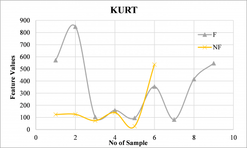
Features map is a graphical distribution of features to visually predict class separability. Figure 4 presents feature maps of two features from the time domain (KURT) and two features from the frequency domain (SNR). From these figures, it could be predicted graphically that was separable with possibilities of two misclassified features. KURT will get one misclassified feature and PSR with all correct classification results. However, this was only applicable to single feature performance prediction. Further investigation on the performance of features was required in order to find the best subset of features.
(a) Kurtosis feature map
(b) SNR feature map
Figure 4. Feature maps
In this section, the performance of the feature data is analysed thoroughly. The performance of every single feature, the frequency-domain versus time-domain features, and finally, the analysis of the performance of all rankings calculated in this work were compared. Initially, the performance of every single feature for all samples was calculated. For the single time-domain feature, the best performing feature was the TM5 with 80% accuracy using the RF classifier. Eight time-domain features that acquired 75% accuracy and their corresponding classifiers were as follows: EWL (SVML), EMAV (LDA), WL (SVML), TM4 (DT), TM6 (NB), CC2 (SVM-RBF), KURT (SVM-RBF) and V4(DT). Eleven time-domain features that had achieved 70% classification accuracy were ZC, SSC, DASDV, LD, MYOP, SSI, MFL, AMAVS, TM3, IEMG, and V3. The remaining fifteen time-domain features scored between 60 and 65%.
The best single frequency-domain features were SNR and PSR, with an 80% accuracy using the LDA and DT classifiers. Seven frequency-domain features had acquired 70% accuracy. These features and their corresponding classifiers were as follows: PKF (NB), MNP (kNN), TTP (kNN), SM1, SM2, SM3, SM4 (NB). The MDF (kNN) and VCF (LDA) had achieved a 65% accuracy. The lowest accuracy was 55%, which was acquired by MNF using the kNN classifier. Single feature classification for drowsiness detection could only achieve the highest accuracy of 80%, regardless of the type of the features, which seemed to be fairly low in detecting driver fatigue for EMG signal.
3.2 First layer feature selection
In the first layer feature selection method, 21 filter algorithms were calculated to acquire a ranking matrix (RM). In search of the best subset of features, for each rank, the features were added iteratively and classified to calculate their accuracy performance. All performance was recorded and the highest accuracy was selected for all filters. Table 4 lists down the performance of the ranking groups, namely RTDF, RFDF and RCF, for all filter rankings as well as the accuracy results for each filter.
Table 4. Classification performance for all rankings
|
Filter Rank |
RFDF |
RTDF |
RCF |
||||||
|
Accuracy |
NOF |
Classifier |
Accuracy |
NOF |
Classifier |
Accuracy |
NOF |
Classifier |
|
|
ECFS |
70 |
1 |
kNN |
85 |
16 |
LDA |
70 |
2 |
NB |
|
Chi-Square |
70 |
1 |
kNN |
75 |
11 |
LDA |
85 |
4 |
NB |
|
DGUFS |
70 |
1 |
NB |
75 |
1 |
SVM-L |
75 |
2 |
SVM-L |
|
Fisher |
75 |
2 |
NB |
85 |
15 |
LDA |
80 |
12 |
LDA |
|
FSASL |
75 |
4 |
NB |
75 |
2 |
DT |
70 |
4 |
kNN |
|
FSCM |
75 |
5 |
NB |
75 |
6 |
NB |
70 |
8 |
LDA |
|
F-Value |
70 |
8 |
NB |
85 |
19 |
LDA |
70 |
1 |
SVM-L |
|
ILFS |
70 |
1 |
NB |
75 |
1 |
NB |
80 |
3 |
DT |
|
InFS |
75 |
2 |
NB |
75 |
8 |
NB |
75 |
2 |
SVM-L |
|
Laplacian |
75 |
2 |
LDA |
80 |
7 |
LDA |
85 |
15 |
LDA |
|
LLCFS |
75 |
8 |
kNN |
75 |
1 |
SVM-L |
75 |
5 |
SVM-L |
|
MCFS |
75 |
4 |
NB |
75 |
4 |
NB |
95 |
16 |
LDA |
|
MRMR |
75 |
5 |
NB |
85 |
15 |
LDA |
85 |
15 |
LDA |
|
MIFS |
75 |
8 |
kNN |
80 |
4 |
LDA |
80 |
15 |
LDA |
|
NCA |
80 |
1 |
LDA |
75 |
1 |
SVM-RBF |
85 |
15 |
LDA |
|
Pearson |
70 |
1 |
kNN |
85 |
5 |
NB |
80 |
2 |
LDA |
|
Relieff |
75 |
2 |
NB |
75 |
2 |
DT |
75 |
1 |
SVM-RBF |
|
Spearman |
80 |
1 |
LDA |
85 |
13 |
LDA |
70 |
2 |
NB |
|
T-test |
75 |
2 |
NB |
85 |
3 |
NB |
80 |
2 |
NB |
|
UDFS |
75 |
2 |
NB |
75 |
3 |
SVM-RBF |
65 |
1 |
SVM-L |
|
UFSOL |
70 |
1 |
NB |
90 |
8 |
LDA |
85 |
13 |
LDA |
*Note - NOF: number of features
For the RFDF ranking group, two filter methods—NCA and Spearman—yielded 80% accuracy with one frequency-domain feature using the LDA classifier. The feature with the highest accuracy for both filters was the SNR feature. This was in agreement with the single frequency-domain feature performance, where the SNR feature had acquired 80% accuracy. The rest of the filter rankings achieved either 75 or 75% accuracy. It was observed that the frequency-domain features alone could not achieve higher than 80% classification accuracy.
The highest accuracy for the RTDF ranking group was achieved by the UFSOL filter, with 90% accuracy for eight time-domain features—SSC, ZC, KURT, EWL, TM3, TM5, AR2, WL, and TM4—using the LDA classifier. Meanwhile, the least number of time-domain features with the highest classification accuracy was three (LD, EWL and AMAVS), which had acquired 85% accuracy using T-test filter ranking. The lowest classification accuracy for eleven time-domain features was acquired by the Chi-Square filter ranking with 70% accuracy using the LDA classifier.
For the combined time-domain and frequency-domain features ranking (RCF), the best classification accuracy achieved was 95% using the MCFS filter method with LDA classifier for sixteen features. These sixteen features included six frequency-domain features and ten time-domain features (AR3, SM2, KURT, CC3, MDF, AR2, CC1, TTP, PKF, AR4, SKEW, AR1, LD, SM1, SM3, and EMAV). The combination of time-domain and frequency-domain features increased the classification accuracy performance by 5%. This classification accuracy was better than that of the previous study that had used the same data, which was only 80% for time-domain features only [18].
For the overall best-performing ranking groups, no one filter method repeatedly stood out as the best FS method for the data. MCFS rank performed the best for combined features, acquiring the highest classification accuracy for all features. MCFS, which analysed the relationship of features in its spectrum domain, had shown that the spectral analysis of the features was more useful than the true values of the features. UFSOL, which had performed with the least subset of features for RTDF, reduced the number of features to eight.
The unsupervised filter methods, namely MCFS and UFSOL, had achieved higher than 90% classification accuracy, which was rarely the case for labelled data. One of the reasons for these results was the fact that in the experiment, the drowsiness level was assessed over a driving duration of two hours. In reality, drowsiness normally occurs within seconds while driving and drivers might not be aware of its occurrence. Therefore, the drivers did not assess their brief periods of drowsiness during the experiment. It was recommended to perform a drowsiness validation that can accurately assess the real state of drowsiness in a shorter duration during driving.
3.3 Second layer feature selection
The second layer of statistical filters, as listed in Table 5, had been applied and the highest accuracy of 95% was achieved using the ASR filter with the LDA classifier on 12 features. The features include SNR, VCF, SM1, PSR, SM3, TM4, MYOP, MAV2, SSI, TM6, AAC and SM4, which were a combination of six time-domain features and six frequency-domain features. The frequency-domain features dominated in the ASR ranking as they were the first five most significant features, followed by six time-domain features and one frequency-domain feature in the last subset of features. Although the second layer statistical rank produced the same accuracy performance, it was better in terms of the least number of features. The ASR performed with four fewer features compared to the subset of features in the RTC ranking group.
Table 5. Statistical rank classification performance
|
Performance\Rank |
ASR |
VSR |
MSR |
MedSR |
|
Accuracy |
95 |
80 |
85 |
70 |
|
NOF |
12 |
8 |
4 |
1 |
|
Classifier |
LDA |
LDA |
NB |
DT |
As ASR calculated the average value rank for all samples and then re-ranked them based on the largest average values, the new rank had identified features that did not cluster close to each other. This second layer rank searched for features that were highly likely to separate well between the two classes. Hence, giving a better classification performance. The second-best performing filter was the MSR rank with 85% accuracy for four features using the NB classifier. The mode statistical rank performed better than the MedSR since it calculated the most repeated ranks of the twenty-one filters. The VSR had performed with 80% accuracy for eight features using the LDA classifier. The lowest accuracy of 70% was achieved by MedSR with one feature using the DT classifier.
With regards to the classification performance of group ranking, the LDA had been consistent in acquiring the highest accuracy. This was due to the predicted feature maps of several features, as shown in Figure 3, where the feature data were almost linearly separable for single feature graphs. Based on all classification performances that had been presented in Sections 3.1 to 3.3, the SNR continuously appeared as one of the best features. However, the ultimate best subset of features in this work was the 12 combined features using the ASR rank method, which had achieved the highest accuracy. The ASR took into account all available rankings for each feature and this procedure was statistically proven to be able to find the best rank. In the RCF group of feature selection, the best subset of features consisted of ten time-domain features and six frequency-domain features. This proved that the time-domain features dominated the best features. Nevertheless, this was not the case when all rankings were taken into account, wherein the ASR statistically ranked eight frequency-domain features, which outnumbered the time-domain features by half. Hence, it is not the case with which features is more meaningful for the best performance, it is the search of best features in both domains. Overall, the new statistical rank produced the best result with the least number of features and high classification accuracy.
In this paper, twenty-one filter methods for feature selection were applied to the EMG raw data for driver fatigue detection and a new statistical rank was proposed. It has been shown that the new statistical rank ASR delivered the best performance as compared to the single filter rank in terms of the least number of the best subset of features. The best subset of features was a combination of frequency-domain and time-domain features. Concurrently, the best single filter method for the EMG signals of driver fatigue, performed with the same classification accuracy compared to ASR, but with more features. The number of features was reduced significantly from 47 to 12 (75% fewer features), which meant less computational time. The proposed model is the potential to the development of a more robust feature filter selection method. In the future, multi validation procedure is desirable for a more accurate drowsiness level validation. Based on the results of the single ranking method, combinations of two or three filter methods might be a promising new algorithm for feature selection.
The authors would like to thank the Ministry of Higher Education for providing financial support under Fundamental Research Grant Scheme (FRGS) No. FRGS/1/2019/TK04/UMP/02/7 (University reference RDU1901167) and Universiti Malaysia Pahang (UMP) for financial support under PGRS grant PGRS210331. The authors also would like to thank UMP for the laboratory facilities.
[1] Kumar, M. (2018). Fatigue, Mobile Phone Use among Top Causes of Road Accidents. The Star Online.
[2] Rahman, N.A.A., Mustafa, M., Samad, R., Abdullah, N.R.H., Sulaiman, N. (2019). Energy spectral density analysis of muscle fatigue. In Proceedings of the 10th National Technical Seminar on Underwater System Technology 2018, pp. 437-446. https://doi.org/10.1007/978-981-13-3708-6_37
[3] Dolezalek, E., Farnan, M., Min, C.H. (2021). Physiological signal monitoring system to analyze driver attentiveness. In 2021 IEEE International Midwest Symposium on Circuits and Systems (MWSCAS), pp. 635-638. https://doi.org/10.1109/MWSCAS47672.2021.9531871
[4] de Naurois, C.J., Bourdin, C., Stratulat, A., Diaz, E., Vercher, J.L. (2019). Detection and prediction of driver drowsiness using artificial neural network models. Accident Analysis & Prevention, 126: 95-104. https://doi.org/10.1016/j.aap.2017.11.038
[5] Akiduki, T., Nagasawa, J., Zhang, Z., Omae, Y., Arakawa, T., Takahashi, H. (2022). Inattentive driving detection using body-worn sensors: Feasibility study. Sensors, 22(1): 352. https://doi.org/10.3390/s22010352
[6] Zahari, Z.L., Mustafa, M., Zain, Z.M., Abdubrani, R., Naim, F. (2021). The enhancement on stress levels based on physiological signal and self-stress assessment. Traitement du Signal, 38(5): 1439-1447. https://doi.org/10.18280/ts.380519
[7] Gangadharan, S., Vinod, A.P. (2022). Drowsiness detection using portable wireless EEG. Computer Methods and Programs in Biomedicine, 214: 106535. https://doi.org/10.1016/j.cmpb.2021.106535
[8] Arefnezhad, S., Samiee, S., Eichberger, A., Nahvi, A. (2019). Driver drowsiness detection based on steering wheel data applying adaptive neuro-fuzzy feature selection. Sensors, 19(943): 1-14. https://doi.org/10.3390/s19040943
[9] Tuncer, T., Dogan, S., Subasi, A. (2021). EEG-based driving fatigue detection using multilevel feature extraction and iterative hybrid feature selection. Biomedical Signal Processing and Control, 68: 102591. https://doi.org/10.1016/j.bspc.2021.102591
[10] Cheng, Q., Wang, W., Jiang, X., Hou, S., Qin, Y. (2019). Assessment of driver mental fatigue using facial landmarks. IEEE Access, 7: 150423-15034. https://doi.org/10.1109/ACCESS.2019.2947692
[11] Moujahid, A., Dornaika, F., Arganda-Carreras, I., Reta, J. (2021). Efficient and compact face descriptor for driver drowsiness detection. Expert Systems with Applications, 168: 114334. https://doi.org/10.1016/j.eswa.2020.114334
[12] Sharanabasappa, Nandyal, S. (2021). An ensemble learning model for driver drowsiness detection and accident prevention using the behavioral features analysis. International Journal of Intelligent Computing and Cybernetics, 15(2): 224-244. https://doi.org/10.1108/IJICC-07-2021-0139
[13] Henni, K., Mezghani, N., Gouin-Vallerand, C., Ruer, P., Ouakrim, Y., Vallières, É. (2018). Feature selection for driving fatigue characterization and detection using visual-and signal-based sensors. Applied Informatics, 5(7): 1-15. https://doi.org/10.1186/s40535-018-0054-9
[14] Liu, X., Zhou, M., Geng, Y., et al. (2021). Changes in synchronization of the motor unit in muscle fatigue condition during the dynamic and isometric contraction in the Biceps Brachii muscle. Neuroscience Letters, 761: 136101. https://doi.org/10.1016/j.neulet.2021.136101
[15] Aiamklin, W., Jewajinda, Y., Punsawad, Y. (2022). Light sleep detection based on surface electromyography signals for nap monitoring. International Journal of Biology and Biomedical Engineering, 16: 140-145. https://doi.org/10.46300/91011.2022.16.18
[16] Satti, A.T., Kim, J., Yi, E., Cho, H.Y., Cho, S. (2021). Microneedle array electrode-based wearable EMG system for detection of driver drowsiness through steering wheel grip. Sensors, 21(15): 5091. https://doi.org/10.3390/s21155091
[17] Campbell, E., Phinyomark, A., Scheme, E. (2020). Current trends and confounding factors in myoelectric control: Limb position and contraction intensity. Sensors, 20(6): 1613. https://doi.org/10.3390/s20061613
[18] Naim, F., Mustafa, M., Sulaiman, N., Rahman, N.A.A. (2022). The study of time domain features of EMG signals for detecting driver’s drowsiness. In Recent Trends in Mechatronics Towards Industry 4.0, 730: 427-438. https://doi.org/10.1007/978-981-33-4597-3_39
[19] Shahid, A., Wilkinson, K., Marcu, S., Shapiro, C.M. (2012). STOP, THAT and One Hundred Other Sleep Scales. Springer Science & Business Media, pp. 161-162.
[20] Englehart, K., Hugdins, B., Parker, P. (2000). Multifunction control of prostheses using the myoelectric signal. Intelligent Systems and Technologies in Rehabilitation Engineering, pp. 153-208.
[21] Too, J., Abdullah, A.R., Saad, N.M. (2019). Classification of hand movements based on discrete wavelet transform and enhanced feature extraction. Int. J. Adv. Comput. Sci. Appl, 10(6): 83-89. https://doi.org/10.14569/IJACSA.2019.0100612
[22] Roffo, G. (2016). Feature selection library (MATLAB toolbox). arXiv preprint arXiv:1607.01327. https://doi.org/10.48550/arXiv.1607.01327
[23] Hudgins, B., Parker, P., Scott, R.N. (1993). A new strategy for multifunction myoelectric control. IEEE Transactions on Biomedical Engineering, 40(1): 82-94. https://doi.org/10.1109/10.204774
[24] Oskoei, M.A., Hu, H. (2008). Support vector machine-based classification scheme for myoelectric control applied to upper limb. IEEE Transactions on Biomedical Engineering, 55(8): 1956-65. https://doi.org/10.1109/TBME.2008.919734
[25] Lei, M., Meng, G. (2012). Nonlinear analysis of surface EMG signals. Computational Intelligence in Electromyography Analysis—A Perspective on Current Applications and Future Challenges, pp. 120-171.
[26] Phinyomark, A., Phukpattaranont, P., Limsakul, C. (2012). Fractal analysis features for weak and single-channel upper-limb EMG signals. Expert Systems with Applications, 39(12): 11156-11163. https://doi.org/10.1016/j.eswa.2012.03.039
[27] Campbell, E., Phinyomark, A., Scheme, E. (2019). Feature extraction and selection for pain recognition using peripheral physiological signals. Frontiers in Neuroscience, 13: 437. https://doi.org/10.3389/fnins.2019.00437
[28] Phinyomark, A., Phukpattaranont, P., Limsakul, C. (2012). Feature reduction and selection for EMG signal classification. Expert Systems with Applications, 39(8): 7420-7431. https://doi.org/10.1016/j.eswa.2012.01.102
[29] Tkach, D., Huang, H., Kuiken, T.A. (2010). Study of stability of time-domain features for electromyographic pattern recognition. Journal of Neuroengineering and Rehabilitation, 7(21): 1-13. https://doi.org/10.1186/1743-0003-7-21
[30] Zardoshti-Kermani, M., Wheeler, B.C., Badie, K., Hashemi, R.M. (1995). EMG feature evaluation for movement control of upper extremity prostheses. IEEE Transactions on Rehabilitation Engineering, 3(4): 324-333. https://doi.org/10.1109/86.481972
[31] Jeong, E.C., Kim, S.J., Song, Y.R., Lee, S.M. (2013). Comparison of wrist motion classification methods using surface electromyogram. Journal of Central South University, 20(4): 960-968. https://doi.org/10.1007/s11771-013-1571-2
[32] Nazarpour, K., Al-Timemy, A.H., Bugmann, G., Jackson, A. (2013). A note on the probability distribution function of the surface electromyogram signal. Brain Research Bulletin, 90(1): 88-91. https://doi.org/10.1016/j.brainresbull.2012.09.012
[33] Westerink, J.H., Broek, E.L., Schut, M.H., Herk, J.V., Tuinenbreijer, K. (2008). Computing emotion awareness through galvanic skin response and facial electromyography. In Probing Experience, pp. 149-62. https://doi.org/10.1007/978-1-4020-6593-4_14
[34] Arjunan, S.P., Kumar, D.K. (2010). Decoding subtle forearm flexions using fractal features of surface electromyogram from single and multiple sensors. Journal of Neuroengineering and Rehabilitation, 7(1): 1-10. https://doi.org/10.1186/1743-0003-7-53
[35] Khushaba, R.N., Al-Ani, A., Al-Jumaily, A. (2010). Orthogonal fuzzy neighborhood discriminant analysis for multifunction myoelectric hand control. IEEE Transactions on Biomedical Engineering, 57(6): 1410-1419. https://doi.org/10.1109/TBME.2009.2039480
[36] Côté-Allard, U., Campbell, E., Phinyomark, A., Laviolette, F., Gosselin, B., Scheme, E. (2020). Interpreting deep learning features for myoelectric control: A comparison with handcrafted features. Frontiers in Bioengineering and Biotechnology, 8: 158. https://doi.org/10.3389/fbioe.2020.00158
[37] Kendell, C., Lemaire, E. D., Losier, Y., Wilson, A., Chan, A., Hudgins, B. (2012). A novel approach to surface electromyography: an exploratory study of electrode-pair selection based on signal characteristics. Journal of Neuroengineering and Rehabilitation, 9(1): 24. https://doi.org/10.1186/1743-0003-9-24
[38] Roffo, G., Melzi, S., Castellani, U., Vinciarelli, A. (2017). Infinite latent feature selection: A probabilistic latent graph-based ranking approach. In Proceedings of the IEEE International Conference on Computer Vision, pp. 1398-1406. https://doi.org/10.1109/ICCV.2017.156
[39] Roffo, G., Melzi, S., Cristani, M. (2015). Infinite feature selection. In Proceedings of the IEEE International Conference on Computer Vision, pp. 4202-4210.
[40] Roffo, G., Melzi, S. (2017). Ranking to learn: Feature ranking and selection via eigenvector centrality, new frontiers in mining complex patterns. In Fifth International Workshop nfMCP2016. https://doi.org/10.1007/978-3-319-61461-8_2
[41] Peng, H., Long, F., Ding, C. (2005). Feature selection based on mutual information criteria of max-dependency, max-relevance, and min-redundancy. IEEE Transactions on Pattern Analysis and Machine Intelligence, 27(8): 1226-1238. https://doi.org/10.1109/TPAMI.2005.159
[42] Kononenko, I. (1994). Estimating attributes: Analysis and extensions of RELIEF. In European Conference on Machine Learning, pp. 171-82. https://doi.org/10.1007/3-540-57868-4_57
[43] Zaffalon, M., Hutter, M. (2002). Robust feature selection by mutual information distributions. arXiv preprint cs/0206006. https://doi.org/10.48550/arXiv.cs/0206006
[44] Bradley, P.S., Mangasarian, O.L. (1998). Feature selection via concave minimization and support vector machines. In ICML, 98: 82-90.
[45] Goldberger, J., Hinton, G.E., Roweis, S., Salakhutdinov, R.R. (2004). Neighbourhood components analysis. Advances in Neural Information Processing Systems.
[46] Gu, Q., Li, Z., Han, J. (2012). Generalized fisher score for feature selection. arXiv preprint arXiv:1202.3725. https://doi.org/10.48550/arXiv.1202.3725
[47] Chormunge, S., Jena, S. (2018). Correlation based feature selection with clustering for high dimensional data. Journal of Electrical Systems and Information Technology, 5(3): 542-549. https://doi.org/10.1016/j.jesit.2017.06.004
[48] Shafiei, S.B., Durrani, M., Jing, Z., et al. (2021). Surgical hand gesture recognition utilizing electroencephalogram as input to the machine learning and network neuroscience algorithms. Sensors, 21(5): 1733. https://doi.org/10.3390/s21051733
[49] Thaseen, I.S., Kumar, C.A. (2017). Intrusion detection model using fusion of chi-square feature selection and multi class SVM. Journal of King Saud University-Computer and Information Sciences, 29(4): 462-72. https://doi.org/10.1016/j.jksuci.2015.12.004
[50] Zhao, H., Yuan, L., Chen, Z., Liao, Y., Lin, J. (2021). Exploring the diagnostic effectiveness for myocardial ischaemia based on CCTA myocardial texture features. BMC Cardiovascular Disorders, 21(1): 1-10. https://doi.org/10.1186/s12872-021-02206-z
[51] Hoffman, J.I.E. (2015). T-test variants: crossover tests, equivalence tests. Biostatistics for Medical and Biomedical Practitioners; Academic Press: Cambridge, MA, USA, pp. 363-371.
[52] He, X., Cai, D., Niyogi, P. (2005). Laplacian score for feature selection. Advances in Neural Information Processing Systems.
[53] Cai, D., Zhang, C., He, X. (2010). Unsupervised feature selection for multi-cluster data. In Proceedings of the 16th ACM SIGKDD International Conference on Knowledge Discovery and Data Mining, pp. 333-342. https://doi.org/10.1145/1835804.1835848
[54] Yang, Y., Shen, H. T., Ma, Z., Huang, Z., Zhou, X. (2011). L2, 1-norm regularized discriminative feature selection for unsupervised. In Twenty-Second International Joint Conference on Artificial Intelligence, pp. 1589-1594.
[55] Zeng, H., Cheung, Y.M. (2010). Feature selection and kernel learning for local learning-based clustering. IEEE Transactions on Pattern Analysis and Machine Intelligence, 33(8): 1532-47. https://doi.org/10.1109/TPAMI.2010.215
[56] Zhou, P., Du, L., Li, X., Shen, Y.D., Qian, Y. (2020). Unsupervised feature selection with adaptive multiple graph learning. Pattern Recognition, 105: 107375. https://doi.org/10.1016/j.patcog.2020.107375
[57] Guo, J., Zhu, W. (2018). Dependence guided unsupervised feature selection. In Proceedings of the AAAI Conference on Artificial Intelligence, pp. 2232-2239. https://ojs.aaai.org/index.php/AAAI/article/view/11904.
[58] Guo, J., Guo, Y., Kong, X., He, R. (2017). Unsupervised feature selection with ordinal locality. In 2017 IEEE International Conference on Multimedia and Expo (ICME), pp. 1213-1218. https://doi.org/10.1109/ICME.2017.8019357
[59] Ghorbanian, A., Maghsoudi, Y., Mohammadzadeh, A. (2020). Clustering-based band selection using structural similarity index and entropy for hyperspectral image classification. Traitement du Signal, 37(5): 785-791. https://doi.org/10.18280/ts.370510
[60] Özyurt, F. (2021). Automatic detection of COVID-19 disease by using transfer learning of light weight deep learning model. Traitement du Signal, 38(1): 147-53. https://doi.org/10.18280/ts.380115
[61] Taran, S., Bajaj, V., Sinha, G.R., Polat, K. (2021). Detection of sleep apnea events using electroencephalogram signals. Applied Acoustics, 181: 108137. https://doi.org/10.1016/j.apacoust.2021.108137
[62] Spiewak, C., Islam, M., Zaman, M.A.U., Rahman, M.H. (2018). A comprehensive study on EMG feature extraction and classifiers. Open Access Journal of Biomedical Engineering and Biosciences, 1(1): 1-10.
[63] Kose, M.R., Ahirwal, M.K., Kumar, A. (2021). A new approach for emotions recognition through EOG and EMG signals. Signal, Image and Video Processing, 15(8): 1863-1871. https://doi.org/10.1007/s11760-021-01942-1
[64] Amrani, M.Z., Borst, C.W., Achour, N. (2022). Multi-sensory assessment for hand pattern recognition. Biomedical Signal Processing and Control, 72: 103368. https://doi.org/10.1016/j.bspc.2021.103368
[65] Bhattacharya, A., Pahari, P., Basak, P., Sarkar, A. (2019). Class discriminator-based EMG classification approach for detection of neuromuscular diseases using discriminator-dependent decision rule (D3R) approach. In Recent Trends in Signal and Image Processing, pp. 49-56. https://doi.org/10.1007/978-981-10-8863-6_6
[66] Khan, S.M., Khan, A.A., Farooq, O. (2021). Pattern recognition of EMG signals for low level grip force classification. Biomedical Physics & Engineering Express, 7(6): 065012. https://doi.org/10.1088/2057-1976/ac2354