Menaka Radhakrishnan* | Swagata Boruah | Karthik Ramamurthy
© 2022 IIETA. This article is published by IIETA and is licensed under the CC BY 4.0 license (http://creativecommons.org/licenses/by/4.0/).
OPEN ACCESS
An electroencephalogram (EEG) test can be utilized to capture the electrical impulses in the human brain. EEG signal analysis is crucial in the detection and treatment of brain diseases. Autism is one of the neurological disorders that needs to be diagnosed in the early stages of life. Autistic behavior is difficult to differentiate and it can even lead to adverse effects in the daily routine of a kid. Recent advances in Artificial Intelligence have proven to be an effective way of diagnosing ASD. This research employs PyCaret framework to analyze the anomalies present in the EEG signal data in the context of differentiating Autistic children from Typically developing children. The different anomaly detection modules have been used to detect anomalies, compute their anomaly scores and visualize it. The goal of this study is to determine if PyCaret's anomaly detection module can aid the detection of ASD.
anomaly detection, PyCaret, ASD, ABOD
Autism Spectrum Disorder (ASD) is a form of developmental disorder used to describe individuals with a specific mix of deficits in social communication and repetitive behaviours, as well as very restricted interests and/or sensory behaviours that begin early in infancy. It is defined by a diverse set of behavioural abnormalities that arise throughout a person's early stages of development. Psychosocial therapies in children can enhance particular behaviours such as joint attention, language, and social engagement, all of which can have an impact on future development and symptom severity. However, more study is needed to determine the long-term requirements of persons with autism, as well as therapies and mechanisms that might lead to improvement in quality of life in the long run [1]. The EEG's potency as a component of brain study continues to expand as new means of evaluating and obtaining information from biophysical signals. Network variability may be seen through time series estimations using methods for analysing complex and intricate networks such as the human brain. As a result, a collection of invariant measures derived from EEG data must represent the neuronal prospects in the brain that generates the signals [2-5]. EEGs are established as observations of electrical activity in the brain acquired from the surface of the scalp. These devices with excellent temporal resolution can monitor brain impulses in milliseconds, providing a lot of data. Graphical analysis can be highly valuable, but it isn't always enough since the volume of data becomes too vast to comprehend. J48 and Random Tree are employed with the band frequency and the Beta band frequency as input [6]. The voltage fluctuations in EEG were analysed using classification based algorithms [7]. These techniques reveal typical or dysfunctional EEG activity that would otherwise be undetectable [8]. Autism features can be detected by screening tests, but they are costly and time consuming. Autism may now be predicted at an early stage due to the advances in Artificial Intelligence. The authors proposed an effective machine learning model that was developed by merging Random Forest-CART and Random Forest-Id3 for detecting normal and autistic traits [9]. Machine learning models were used to predict ASD diagnoses and ADOS-2 scores, which offered an approximation of the presence of long and short term tendencies [10]. According to the findings in the study [11], a small portion of EEG provides valuable information that can be used to identify autism if it is processed using modern computer techniques like machine learning. Machine learning algorithms can handle a lot of data. They do it as part of their on going hunt for critical decision-making connections. There is an enormous quantity of material to be discussed in the realm of medical diagnosis [12]. As a result, spotting outliers in a complicated data environment is critical in both science and engineering. However, when data streams vary over time, standard approaches become ineffective, necessitating the use of an outlier identification algorithm that can handle dynamic data streams. PyCaret is a Python machine learning package that automates machine learning operations and is open-source [13]. Low-code autoML framework PyCaret (automatic machine learning) can be utilized to enhance data for a variety of applications, but there is a dearth of expertise about them. In this study, we will be using PyCaret’s anomaly detection module to analyse our data.
The work flow process followed for this study has been depicted in Figure 1.
2.1 EEG data acquisition
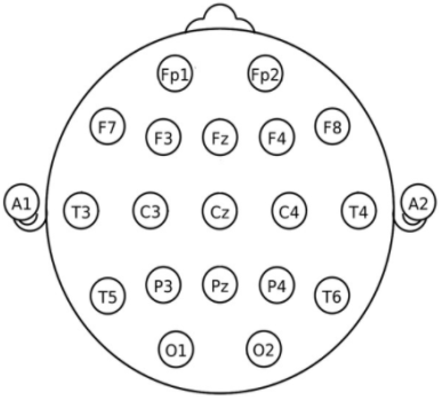
The collection of raw data is the first stage in processing any type of signal. The signals were collected at a frequency of 500 Hz. EEG montage describes the practice of taking EEG readings as a relative metric. Bipolar, Laplacian, common electrode reference, average, and weighted averaged references are among the several montages [8]. EEG data was gathered with average reference electrodes for this study. Participants in the study ranged in age from 3 to 7. For each individual, a total of 10,000 EEG signal samples were obtained from each of the 19 distinct EEG channels which were then used for training. The first 10,000 sample points of EEG data for all children were chosen as the sample points. Because each kid had a varied set of sample points recorded, ranging from 10,000 to 15,000, the first 10,000 data points were picked for everyone to guarantee that the number of sample points was consistent. During the course of the acquisition, the participants were given visual stimuli. The International 10-20 system of electrode placement positions has been endorsed. Figure 2 shows the pictorial representation of the electrode placement. The positions were Fp1, Fp2, F7, F3, Fz, F4, F8, P3, P4, Pz, T3, T5, T4, T6, O1, O2, C3, C4 and Cz [14-19].
Figure 1. Workflow of the proposed work
Figure 2. International 10-20 system of EEG. Electrode placement
In total, there were 6 EEG signal datasets used in this study, out of which 3 belong to typically developing children (TD) and 3 belong to children with autism spectrum disorder (AD). The output of each channel is digitized and stored as comma separated values (.CSV format). These datasets were used in their original form for performing spatial analysis which helps to determine the time stamp of occurrence of anomalies. Then this dataset was transposed for performing time analysis which helps in identifying particular channels in the EEG signal which have different behavior than other channels. Furthermore, these datasets were fed into PyCaret’s Anomaly detection models, namely ABOD, Isolation forest and MCD which have been discussed in detailed in section 2.2.
2.2 PyCaret – anomaly detection module
PyCaret is a Python-based machine learning framework for automating machine learning workflows [11, 13]. Anomaly detection is the process of discovering unusual things, events, or observations that raise concerns because they differ significantly from the overall set of data points. Here in this study, we have utilized the anomaly detection module, namely Angle-based Outlier Detector, Isolation Forest and Minimum Covariance Determinant models which have been discussed below:
2.2.1 Angle-based outlier detection (ABOD)
The ABOD model allots the Angle-based Outlier Factor (ABOF) to each point in the dataset and the result is a list of points sorted according to this factor. The divergence in orientations of objects when compared to each other is described by an ABOF. We compute the scalar product of the difference vectors of any triple of points with a normalization process. This is carried out by determining the quadratic product of the length of the difference vectors. The distance does impact the value, but only to a little extent, because of this weighting component [19-21]. In short, given a dataset $\mathrm{D} \subseteq \mathbb{R}^{\mathrm{d}}$, a point $\overrightarrow{\mathrm{L}} \in \mathrm{D}$, and a norm $\|.\|: \mathbb{R}^{\mathrm{d}} \rightarrow \mathbb{R}^{\mathrm{d}_{0}}$. The scalar product is denoted by $\langle., .\rangle: \mathbb{R}^{\mathrm{d}} \times \mathbb{R}^{\mathrm{d}} \rightarrow \mathbb{R}$. For two points $\overrightarrow{\mathrm{M}}, \overrightarrow{\mathrm{N}} \in$ $\mathrm{D}, \overline{\mathrm{MN}}$ denotes the difference vector $\overrightarrow{\mathrm{M}}-\overrightarrow{\mathrm{N}}$. The $\mathrm{ABOF}(\overrightarrow{\mathrm{L}})$ is the variance over the angles between the difference vectors of $\overrightarrow{\mathrm{L}}$ to all pairs of points in D weighted by the distance of the points [22, 23].
2.2.2 Isolation forest
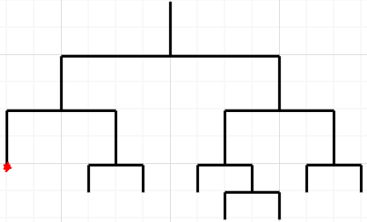
Isolation forest internally uses the concept of decisions trees. Here, a tree structure is generated based on randomly drawn attributes from the sub-sampled information, which is then analyzed by the isolation forest. Anomalies are much less likely to occur in samples that travel further down the tree since they require more cuts to isolate them. Similarly, samples that end up in shorter branches suggest anomalies since the tree had an easier time distinguishing them from other data. There are two stages in this process, firstly it builds isolation trees based on sub samples of the data and then these instances are tested through isolation trees to assign an anomaly score to each data point [24-26]. The process of building the tree is given below and illustrated in Figure 3.
Let X={x1, …, xn} be a set of d-dimensional points and $X^{\prime} \subset X$ Any Isolation Tree data structure can be described by the following characteristics:
1. For every node N in the tree, N can either be an external node with no child or an internal-node with one “test” and exactly two daughter nodes (Nleft and Nright).
2. A test at node N comprises of an attribute a and split value b such that a<b which will determine the traversal of the data point towards either Nleftor Nright.
Figure 3. Structure of the spanning tree – red dot is the anomalous data point
The algorithm recursively splits X' by randomly selecting a and b in order to build the isolation (iTree) until either of the following scenarios is incurred:
1. There is only one instance of the node.
2. Every data point in the particular node has same values.
Once this tree is fully constructed, every element in X is isolated at one of the external nodes. Hence, anomalous data points are those with the smaller path length in the tree, where the path length p(xi) of point $x_{i} \in X$ is defined as the number of edges traversed from the root node to get to an external node by xi. In other words, while scoring, the data point is navigated through all the trees which have been trained earlier. These scores are assigned based on the depth of the particular tree required to reach that particular point. The depth acquired from each of the Isolation Trees is combined to produce this score and the data points which have the smallest path length are taken as the anomalous data point.
2.2.3 Minimum covariance determinant (MCD)
Minimum Covariance Determinant is a technique for assessing the mean and covariance matrix by locating data points with the lowest determinants in the Covariance matrix. To put it another way, the covariance matrix is utilized as a distinguishing parameter to determine if data points are outliers or not [25-32]. The MCD estimator can be described as ($\hat{\mu}_{0}, \widehat{\Sigma}_{0}$) having a tuning constant n/2≤h≤n where,
1. $\hat{\mu}_{0}$ is the mean of h data points for which the determinant value of this sample’s covariance matrix is as low as possible. This is known as the location estimate.
2. $\widehat{\Sigma}_{0}$ is the corresponding covariance matrix multiplied by constant c0 (consistency factor). This is known as the scatter matrix estimate.
This MCD estimator (μ^MCD,∑^MCD) has been given below as Eq. (1) where $d_{i}=d\left(x, \hat{\mu}_{0}, \widehat{\sum}_{0}\right)$ and W is a weight function of choice. W is set to 1 if the distance is less than a threshold √x2p,0.975 and 0 otherwise [33-36]. ${x}_{i}$ is the particular data point and constant ${c}_{i}$ is a consistency factor.
$\mu_{M C D}=\frac{\sum_{i=1}^{n} W\left(d_{i}^{2}\right) x_{i}}{\sum_{i=1}^{n} W\left(d_{i}^{2}\right)}$
$\sum^{\wedge}{ }_{M C D}=c_{1} \frac{1}{n} \sum_{i=1}^{n} W\left(d_{i}^{2}\right)\left(x_{i}-\mu^{\wedge}{ }_{M C D}\right)\left(x_{i}-\mu^{\wedge}{ }_{M C D}\right)$ (1)
3.1 Spatial analysis for TD and AD groups
In total, six subjects were analyzed, out of which 3 were TD and 3 were diagnosed ASD. Each subject’s EEG data was fed into the three outlier detection models considered for this study. The red dots imply that, the particular data point has been identified as an anomaly by that model. The X-axis denotes the time/duration for which the EEG data was collected and Y-axis denotes the resultant anomaly scores produced by the models. These graphs show the distribution of anomaly scores with respect to time i.e., in which particular time duration anomaly can be detected. The anomaly score graphs for each model were then analyzed.
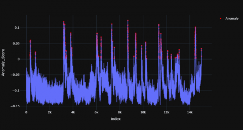
3.1.1 Graphs produced by ABOD model
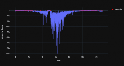
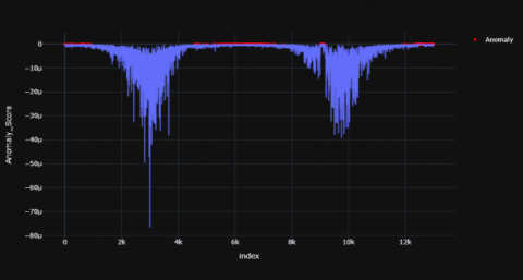
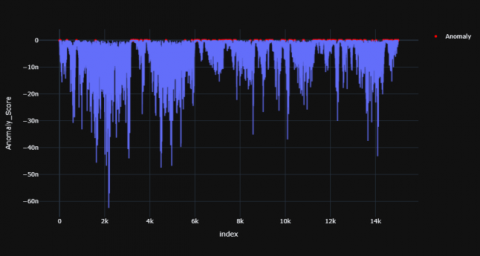
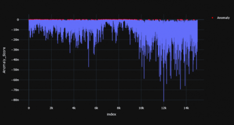
Figures 4-6 shows the resultant anomaly scores graphs for TD child and Figures 7-9 shows the resultant graphs for AD child which were produced using ABOD model.
Figure 4. TD subject -1
Figure 5. TD subject -2
Figure 6. TD subject -3
Figure 7. AD subject -1
Figure 8. AD subject -2
Figure 9. AD subject -3
Table 1. Mean, median and standard deviation of anomaly scores for each TD subject using ABOD
|
S. no. |
Mean |
Median |
Std Dev |
|
1 |
-3.06×10⁻⁶ |
-8.31×10⁻⁷ |
5.46×10⁻⁶ |
|
2 |
-4.06×10⁻⁶ |
-1.35×10⁻⁶ |
6.23×10⁻⁶ |
|
3 |
-2.97×10⁻⁶ |
-1.04×10⁻⁶ |
4.67×10⁻⁶ |
Table 2. Mean, median and standard deviation of anomaly scores for each AD subject using ABOD
|
S. no. |
Mean |
Median |
Std Dev |
|
1 |
-6.47×10⁻⁹ |
-4.47×10⁻⁹ |
6.7×10⁻⁹ |
|
2 |
-3.96×10⁻⁹ |
-2.39×10⁻⁹ |
4.78×10⁻⁹ |
|
3 |
-5.33×10⁻⁹ |
-3.37×10⁻⁹ |
6.03×10⁻⁹ |
In the case of TD child, these red dots (anomaly) have been visible in certain parts of time range but in AD child the anomalies are more scattered and larger in number. In a TD child the anomaly scores have visible peaks at the 2000th, 6000th, 10000th time stamp while there are more numbers of peaks scattered across the time period in the AD child. The red dots represent the anomalous points recognized by the model. For TD child, the anomaly points mostly arise at certain time stamps of the signal whereas their anomalous data points are scattered throughout the time period in an AD child. Overall, there seems to be fewer peaks at specific time stamps in a TD child whereas these peaks are scattered throughout for the AD child. The distribution of the anomaly points has been summarized in Tables 1 and 2.
It was observed that mean, median and standard deviation values of AD child were greater (since the numbers are in negative) when compared to the TD child. The percentage variation of mean, median and standard deviation of a TD child when compared to AD child is 199.38%, 199.62% and 199.57% respectively.
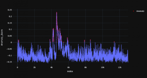
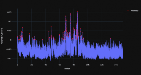
3.1.2 Analysis with isolation forest model
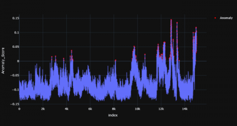
Figures 10-12 shows the resultant anomaly scores graphs for TD child and Figures 13-15 shows the resultant graphs for AD child which were produced using Isolation Forest model.
Figure 10. TD subject -1
Figure 11. TD subject -2
Figure 12. TD subject -3
Figure 13. AD subject -1
Figure 14. AD subject -2
Figure 15. AD subject -3
There are few peaks in the TD subject in the initial time stamp and towards the end i.e. from 0-2k range and 9-12k range. Once there is a peak, it settles down after some time whereas for AD subjects peaks occur multiple times throughout the entire time range and do not settle down even after it occurs. The range of anomaly scores for TD child is between -0.2 to -0.25 whereas the range for an AD child is between -0.15 to 0.15. There are multiple anomalous peaks in the AD child’s graph which is scattered throughout the time period whereas there are fewer visible peaks which have in the TD child. The distribution of the anomaly points has been summed up in Tables 3 and 4.
Table 3. Mean, median and standard deviation of anomaly scores for each td subject using iforest
|
S. no. |
Mean |
Median |
Std Dev |
|
1 |
-0.093 |
-0.106 |
0.049 |
|
2 |
-0.125 |
-0.144 |
0.058 |
|
3 |
-0.097 |
-0.111 |
0.052 |
Table 4. Mean, median and standard deviation of anomaly scores for each AD subject using iforest
|
S. no. |
Mean |
Median |
Std Dev |
|
1 |
-0.077 |
-0.087 |
0.049 |
|
2 |
-0.091 |
-0.103 |
0.058 |
|
3 |
-0.052 |
-0.059 |
0.052 |
3.1.3 Analysis with minimum covariance determinant model
Figure 16. TD subject -1
Figure 17. TD subject -2
Figure 18. TD subject -3
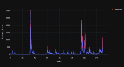
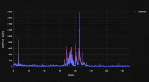
Figure 19. AD subject -1
Figure 20. AD subject -2
Figure 21. AD subject -3
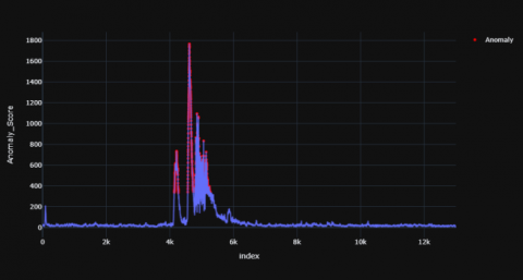
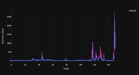
Figures 16-18 shows the resultant anomaly scores graphs for TD child and Figures 19-21 shows the resultant graphs for AD child which were produced using Minimum Covariance Determinant model.
In case of AD child, anomalous peaks have been identified at the positions 7-9k and 12-14k time range. The peak values for AD were 1800, 2500 and 3000 which are significantly higher values than that of TD child’s peak values. The peaks values for TD were 1800, 2000 and 800 for each subject respectively. The range of anomaly scores vary from 0 to a maximum of 3000 in the AD child whereas the peaks have a lower maximum value for the TD child. The distribution of the anomaly points has been summarized in Table 5 and 6.
Table 5. Mean, median and standard deviation of anomaly scores for each TD subject using MCD
|
S. no. |
Mean |
Median |
Std Dev |
|
1 |
64.84 |
21.05 |
159.14 |
|
2 |
59.66 |
21.78 |
118.17 |
|
3 |
51.02 |
22.01 |
94.06 |
Table 6. Mean, median and standard deviation of anomaly scores for each AD subject using MCD
|
S. no. |
Mean |
Median |
Std Dev |
|
1 |
60.26 |
22.98 |
154.29 |
|
2 |
100.27 |
26.44 |
222.85 |
|
3 |
47.90 |
21.99 |
77.31 |
3.2 Resultant graphs for TD and AD for time analysis
There are 19 channels in the EEG signal namely Fp1, Fp2, F7, F3, Fz, F4, F8, P3, P4, Pz, T3, T5, T4, T6, O1, O2, C3, C4 and Cz from which the data was being collected. Here, the dataset was transposed in order to analyze the anomaly scores of each channel in a particular subject. The x axis denotes the time/duration for which the EEG data was collected and y axis denotes the resultant anomaly scores.
3.2.1 Results produced by ABOD model
For the TD child, the channels F7 and F8 have been identified as anomalies whereas for AD child, the channels T5, Fp2 and Pz have been detected as an anomaly with the following anomaly scores summarized in Tables 7 and 8.
Table 7. Depicting the channels in TD child identified as anomaly and respective anomaly score
|
Subject |
Channel |
Anomaly Score |
|
1 |
F7 |
- 7.78×10⁻¹⁸ |
|
2 |
F8 |
-1.82×10⁻¹⁷ |
|
3 |
F7 |
-7.40 X 10⁻¹⁸ |
Table 8. Depicting the channels in AD child identified as anomaly and respective anomaly score
|
Subject |
Channel |
Anomaly Score |
|
1 |
T5 |
- 3.79×10⁻¹⁸ |
|
2 |
Fp2 |
-2.89×10⁻¹⁹ |
|
3 |
Pz |
-6.12×10⁻¹⁹ |
3.2.2 Results produced by isolation forest model
For all AD child the anomalies have been detected in Pz channel whereas for TD the anomalies are detected in FP1 channel with the anomaly scores summarized in Tables 9 and 10.
Table 9. Depicting the channels in TD child identified as anomaly and respective anomaly score
|
Subject |
Channel |
Anomaly Score |
|
1 |
F7 |
2.66×10⁻⁴ |
|
2 |
F7 |
0.0549 |
|
3 |
F7 |
0.0088 |
Table 10. Depicting the channels in AD child identified as anomaly and respective anomaly score
|
Subject |
Channel |
Anomaly Score |
|
1 |
Pz |
0.1019 |
|
2 |
Pz |
0.1298 |
|
3 |
Pz |
0.1183 |
3.2.3 Results produced by minimum covariance determinant model
For the TD subjects, channels T5 and F7 have anomaly whereas in AD subject the anomaly has been detected in channels Fp2, Pz and P3 with the anomaly scores summarized in Tables 11 and 12. It was observed that the abnormal score does not vary from child to child, but there is a small range difference in the anomaly scores of ASD when compared to TD child. There was a percentage difference of 171.44% between the anomaly score of TD and AD child produced by ABOD model. While there was a 138.13% difference in anomaly scores when produced by Isolation Forest model. Whereas there was neither a anomaly score difference nor a significant range difference in anomaly scores produced by the MCD model.
Table 11. Depicting the channels in TD child identified as anomaly and respective anomaly score
|
Subject |
Channel |
Anomaly Score |
|
1 |
T5 |
18 |
|
2 |
F7 |
18 |
|
3 |
T5 |
18 |
Table 12. Depicting the channels in AD child identified as anomaly and respective anomaly score
|
Subject |
Channel |
Anomaly Score |
|
1 |
Fp2 |
18 |
|
2 |
P3 |
18 |
|
3 |
Pz |
18 |
In a TD child, the anomaly is observed in the F7 channel which is not the case for AD child. For the AD child anomalies have been detected in the Pz and Fp2 channels. So the variation in the signal for audio and audio visual stimuli is observed in F7 in TD child and in other regions in AD child.
Therefore, through the spatial analysis we observed that on an average, a TD child’s resultant anomaly score graphs have lesser peaks which settles down/ recedes immediately after the peak occurs. Whereas, for an AD child multiple peaks have been observed throughout the time range and they do not recede with time. Furthermore, by comparing the mean, median and standard deviation of the anomaly scores for a TD and AD we can predict that regions having similar distribution metrics will behave similarly. Through time analysis we can decipher that in a TD child anomaly was detected in F7 channel and in other regions in the AD child. Hence, wherever variation was observed by the particular outlier detection model, we can predict and conjugate the reason for the same.
Anomaly detection can be an effective way of discovering unusual events, or observations that raise concerns in a data.
In this study, we have used PyCaret’s Anomaly Detection Module to analyze the EEG patterns of Autistic children for Visual stimuli. Although there are many anomaly detection methods in this module, here we have used Angle-based Outlier Detector, Isolation Forest and Minimum Covariance Determinant models. In total, 6 child subjects EEG signal data were used, out of which 3 were typically developing (TD) children and 3 were children with Autism Spectrum Disorder (ASD). Through spatial analysis, anomaly scores were generated and their occurrence throughout the time stamp was observed. Through time analysis, variation in the signal for audio and audio visual stimuli behaviour was observed in different channels of the EEG signal. These results were then used to essentially distinguish between a normal child and a child with autistic spectrum disorder. The gathering of EEG data from other subjects on a much greater scale for variability and the usage of alternative outlier detection models from PyCaret's Anomaly Detection Module could be possible future directions. These models can be further fine-tuned with sufficiently larger datasets to improve the credibility of the results and enable the possible real-world deployment of these models.
The Department of Science and Technology (DST) financed this study under the Science for Equity, Empowerment, and Development (SEED) Division (File No: SEED/TIDE/092/2016). We'd like to take this opportunity to express to the Sri Ramachandra Institute of Higher Education and Research for their invaluable guidance and cooperation with data collection.
[1] Lord, C., Risi, S., DiLavore, P.S., Shulman, C., Thurm, A., Pickles, A. (2006). Autism from 2 to 9 years of age. Archives of General Psychiatry, 63(6): 694-701. https://doi.org/10.1001/archpsyc.63.6.694
[2] Irimiciuc, S.A., Zala, A., Dimitriu, D., et al. (2021). Novel approach for EEG signal analysis in a multifractal paradigm of motions. Epileptic and Eclamptic Seizures as Scale Transitions. Symmetry, 13(6): 1024. https://doi.org/10.3390/sym13061024
[3] Lord, C., Elsabbagh, M., Baird, G., Veenstra-Vanderweele, J. (2018). Autism spectrum disorder. The lancet, 392(10146): 508-520. https://doi.org/10.1016/S0140-6736(18)31129-2
[4] Radhakrishnan, M., Ramamurthy, K., Choudhury, K.K., Won, D., Manoharan, T.A. (2021). Performance analysis of deep learning models for detection of autism spectrum disorder from EEG signals. Traitement du Signal, 38(3): 853-863. https://doi.org/10.18280/ts.380332
[5] Radhakrishnan, M., Ramamurthy, K., Kothandaraman, A., Madaan, G., Machavaram, H. (2021). Investigating EEG signals of autistic individuals using detrended fluctuation analysis. Traitement du Signal, 38(5): 1515-1520. https://doi.org/10.18280/ts.380528
[6] Bastos, N.S., Marques, B.P., Adamatti, D.F., Billa, C.Z. (2020). Analyzing EEG signals using decision trees: A study of modulation of amplitude. Computational Intelligence and Neuroscience, 2020: 3598416. https://doi.org/10.1155/2020/3598416
[7] Al-Galal, S.A., Alshaikhli, I.F.T. (2017). Analyzing brainwaves while listening to quranic recitation compared with listening to music based on EEG signals. International Journal on Perceptive and Cognitive Computing, 3(1): 43. https://doi.org/10.31436/ijpcc.v3i1.43
[8] Electroencephalography (EEG) (2022). https://www.ed.ac.uk/clinical-sciences/edinburgh-imaging/research/themes-and-topics/medical-physics/imaging-techniques/electroencephalography, accessed on 26 Feb. 2022.
[9] Omar, K.S., Mondal, P., Khan, N.S., Rizvi, M.R.K., Islam, M.N. (2019). A machine learning approach to predict autism spectrum disorder. In 2019 International Conference on Electrical, Computer and Communication Engineering (ECCE), Cox'sBazar, Bangladesh, pp. 1-6. https://doi.org/10.1109/ECACE.2019.8679454
[10] Jayawardana, Y., Jaime, M., Jayarathna, S. (2019). Analysis of temporal relationships between ASD and brain activity through EEG and machine learning. In 2019 IEEE 20th International Conference on Information Reuse and Integration for Data Science (IRI), Angeles, CA, USA, pp. 151-158. https://doi.org/10.1109/IRI.2019.00035
[11] Grossi, E., Valbusa, G., Buscema, M. (2021). Detection of an autism EEG signature from only two EEG channels through features extraction and advanced machine learning analysis. Clinical EEG and Neuroscience, 52(5): 330-337. https://doi.org/10.1177/1550059420982424
[12] Panesar, A. (2021). Machine learning algorithms. Machine Learning and AI for Healthcare, pp. 85-144. Apress, Berkeley, CA. https://doi.org/10.1007/978-1-4842-6537-6_4
[13] Gain, U., Hotti, V. (2021). Low-code AutoML-augmented data pipeline–a review and experiments. In Journal of Physics: Conference Series, 1828(1): 012015. https://doi.org/10.1088/1742-6596/1828/1/012015
[14] Rojas, G.M., Alvarez, C., Montoya, C.E., De la Iglesia-Vaya, M., Cisternas, J.E., Gálvez, M. (2018). Study of resting-state functional connectivity networks using EEG electrodes position as seed. Frontiers in Neuroscience, 12: 235. https://doi.org/10.3389/fnins.2018.00235
[15] Agcaoglu, O., Miller, R., Mayer, A.R., Hugdahl, K., Calhoun, V.D. (2015). Lateralization of resting state networks and relationship to age and gender. Neuroimage, 104: 310-325. https://doi.org/10.1016/j.neuroimage.2014.09.001
[16] Beckmann, C.F., Smith, S.M. (2004). Probabilistic independent component analysis for functional magnetic resonance imaging. IEEE Transactions on Medical Imaging, 23(2): 137-152. https://doi.org/10.1098/rstb.2005.1634.
[17] Ebersole, J.S., Pedley, T.A. (Eds.). (2003). Current Practice of Clinical Electroencephalography. Lippincott Williams & Wilkins.
[18] Gotman, J., Bénar, C.G., Dubeau, F. (2004). Combining EEG and FMRI in epilepsy: Methodological challenges and clinical results. Journal of Clinical Neurophysiology, 21(4): 229-240. https://doi.org/10.1097/01.WNP.0000139658.92878.2A
[19] Lacruz, M.E., Garcia Seoane, J.J., Valentin, A., Selway, R., Alarcon, G. (2007). Frontal and temporal functional connections of the living human brain. European Journal of Neuroscience, 26(5): 1357-1370. https://doi.org/10.1111/j.1460-9568.2007.05730.x
[20] PyCaret - pycaret 2.3.5 documentation. (2022). https://pycaret.readthedocs.io/en/latest/index.html, accessed on 27 Feb. 2022.
[21] Kriegel, H.P., Schubert, M., Zimek, A. (2008, August). Angle-based outlier detection in high-dimensional data. In Proceedings of the 14th ACM SIGKDD International Conference on Knowledge Discovery and Data Mining, Las Vegas Nevada, USA, pp. 444-452. https://doi.org/10.1145/1401890.1401946
[22] Li, X., Lv, J.C., Cheng, D. (2015). Angle-based outlier detection algorithm with more stable relationships. In Proceedings of the 18th Asia Pacific Symposium on Intelligent and Evolutionary Systems, Volume 1, pp. 433-446. https://doi.org/10.1007/978-3-319-13359-1_34
[23] Shou, Z., Tian, H., Li, S., Zou, F. (2018). Outlier detection with enhanced angle-based outlier factor in high-dimensional data stream. International Journal of Innovative Computing, Information and Control, 14(5): 1633-1651. https://doi.org/10.24507/ijicic.14.05.1633
[24] Liu, F.T., Ting, K.M., Zhou, Z.H. (2012). Isolation-based anomaly detection. ACM Transactions on Knowledge Discovery from Data (TKDD), 6(1): 3. https://doi.org/10.1145/2133360.2133363
[25] Liu, F.T., Ting, K.M., Zhou, Z.H. (2008). Isolation forest. In 2008 Eighth IEEE International Conference on Data Mining, Pisa, Italy, pp. 413-422. https://doi.org/10.1109/ICDM.2008.17
[26] Isolation forest. (2022). https://en.wikipedia.org/w/index.php?title=Isolation_forest&oldid=1068857144, accessed on 27 Feb. 2022.
[27] Rousseeuw, P.J., Driessen, K.V. (1999). A fast algorithm for the minimum covariance determinant estimator. Technometrics, 41(3): 212-223.
[28] Hardin, J., Rocke, D M. (2004). Outlier detection in the multiple cluster setting using the minimum covariance determinant estimator. Computational Statistics & Data Analysis, 44(4): 625-638. https://doi.org/10.1016/S0167-9473(02)00280-3
[29] Hubert, M., Debruyne, M. (2010). Minimum covariance determinant. Wiley Interdisciplinary Reviews: Computational Statistics, 2(1): 36-43. https://doi.org/10.1002/wics.61
[30] Fauconnier, C., Haesbroeck, G. (2009). Outliers detection with the minimum covariance determinant estimator in practice. Statistical Methodology, 6(4): 363-379. https://doi.org/10.1016/j.stamet.2008.12.005
[31] Hubert, M., Debruyne, M., Rousseeuw, P.J. (2018). Minimum covariance determinant and extensions. Wiley Interdisciplinary Reviews: Computational Statistics, 10(3): e1421.https://doi.org/10.1002/wics.1421.
[32] Ghorbani, H. (2019). Mahalanobis distance and its application for detecting multivariate outliers. Facta Univ Ser Math Inform, 34(3): 583-595. https://doi.org/10.22190/FUMI1903583G
[33] Croux, C., Haesbroeck, G. (1999). Influence function and efficiency of the minimum covariance determinant scatter matrix estimator. Journal of Multivariate Analysis, 71(2): 161-190. https://doi.org/10.1006/jmva.1999.1839
[34] Lopuhaa, H.P. (1999). Asymptotics of reweighted estimators of multivariate location and scatter. Annals of Statistics, 27(5):1638-1665.
[35] Pison, G., Van Aelst, S., Willems, G. (2002). Small sample corrections for LTS and MCD. Metrika, 55(1): 111-123. https://doi.org/10.1007/s001840200191
[36] Butler, R.W., Davies, P.L., Jhun, M. (1993). Asymptotics for the minimum covariance determinant estimator. The Annals of Statistics, 21(3): 1385-1400.