Xuan Zheng | Lei Wang | Haijun Zhou*
© 2022 IIETA. This article is published by IIETA and is licensed under the CC BY 4.0 license (http://creativecommons.org/licenses/by/4.0/).
OPEN ACCESS
Focusing on the feature extraction process of convolutional neural network (CNN), this paper establishes a CNN-based retrieval method of book pages. Then, the pretraining and feature finetuning of the CNN were described separately. The performance of the proposed optimization method was demonstrated through experiments. Considering overall performance and transfer learning capacity, the eight-layer VGG-Fast was selected as the structural framework of our CNN. To train the CNN, it is necessary to gather millions of book page images, and complete the complex task of labeling all these images. Given the excellence of VGG in many transfer learning tasks, this paper chooses to pretrain the CNN with a task-independent dataset. After that, a small book page dataset was adopted to convert the knowledge domain of the CNN from image classification to image page retrieval. In this way, desirable retrieval effects were achieved, without wasting lots of time and energy in collecting and labeling a large book page dataset.
convolutional neural network (CNN), image labeling, image page retrieval, VGG-Fast
The research of image retrieval can be traced back to the 1970s. The earliest image retrieval technology is the fast and efficient text-based image retrieval (TBIR): Firstly, the original images are labeled manually, forming several keywords about image contents. Then, the user searches for images in the same way as he/she searches for texts. By entering the keywords/descriptors of the desired image, the relevant images are identified based on the matching degree between texts [1].
As our society is increasingly informatized and networked, however, several defects of TBIR have surfaced: (1) Manual labeling is too costly facing the massive number of images; (2) The image labels are highly subjective, because people differ in cognition and cultural background; (3) A few keywords do not necessarily reflect the rich information embed in an image [2-5]. To sum up, TBIR faces problems like the heavy load of manual labeling, and the subjectiveness of labels. Content-based image retrieval (CBIR), another popular image retrieval technology, is jeopardized by the semantic gap problem.
To overcome the shortcomings of TBIR and CBIR, semantic-based image retrieval (SBIR) was proposed. The key of SBIR is to establish the correlations between the high-level semantic information and low-level visual features of images, thereby fusing the visual and semantic information. As a result, SBIR is also referred to by some scholars as the two-phase fusion image retrieval technology [6]. However, the retrieval strategy of SBIR is essentially the same as that of TBIR and CBIR. SBIR still searches for images by keywords, images, or the combination between them. The difference is that SBIR represents features based on both text semantics and visual features. The combination between image semantics and visual information significantly improves the performance of image retrieval, and boasts great practical and application values [7].
Although machine learning has been extensively applied to image semantic learning, there is no universally applicable image semantic learning method, calling for better learning accuracy for image semantics [8-10]. Drawing on various previous studies, this paper firstly introduces the structure of a self-deigned convolutional neural network (CNN), with a special focus on the feature extraction process of the network. Then, the pretraining and finetuning of the CNN were introduced in details. Finally, the proposed optimization method was verified through experiments.
Giving full consideration to performance and transfer learning ability, this paper chooses the eight-layer VGG-Fast network as the structural framework of our CNN [11-13]. The training of the CNN requires the collection and complex labeling of millions of book page images. Considering the excellence of VGG in many transfer learning tasks, the authors pretrained the CNN with a task-independent dataset. After that, a small book page dataset was adopted to convert the knowledge domain of the CNN from image classification to image page retrieval [14, 15]. In this way, desirable retrieval effects were achieved, without wasting lots of time and energy in collecting and labeling a large book page dataset.
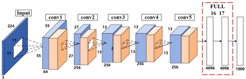
To realize powerful expression of image features, the eight-layer VGG-Fast network was selected as the structure of our CNN, in the light of both performance and transfer learning ability. On 2014 ILSVRC competition, the eight-layer VGG-Fast network finished first in the positioning task, and second in the classification task [16-18]. The Top-5 error of the network on images of 1,000 classes was merely 7.3%, only 0.6% higher than that of the best network. Despite the slight lag in classification error, the VGG network achieved the best results on many transfer learning tasks. Figure 1 shows the structure of the pretrained CNN network [19-21].
As shown in Figure 1, our CNN encompasses an input layer, convolutional layers, pooling layers, rectified linear units (ReLUs), Dropout layers, and fully-connected layers. Specifically, the first convolutional layer (conv1) adopts a kernel size of 11×11 with the sliding step length (stride) of 4 over the feature map. The second convolutional layer (conv2) adopts a kernel size of 5×5 with a stride of 1, and a feature map edge extension (pad) of 2. The third to fifth convolutional layers (conv3-conv5) have the same parameters: kernel size of 3×3, stride of 1, and pad of 1. A pooling layer is arranged after each of conv1, conv2, and conv5 to reduce the dimensionality of features. All three pooling layers adopt the max pooling structure with the kernel size of 3×3, and the stride of 2. In addition, each convolutional layer is followed by an activation function ReLU: ReLU(x)-max(O, x), with x being the input. ReLU does better in one-sided suppression and sparsity than another popular activation function: sigmoid. It can effectively mitigate exploding gradients and vanishing gradients in backpropagation. The last part of the network is two fully-connected layers F6 and F7, whose dimensionality is 4,096, plus a 1,000-dimensional output layer F8, which is also a fully-connected layer. The dimensionality of F8 can be adjusted according to the output class. Table 1 lists the specific parameters.
2.1 CNN pretraining
Through end-to-end training, CNN can fully characterize the visual features of images benefits. It is necessary to train the CNN with a dataset containing millions and even tens of millions of targets. When it comes to book page retrieval, millions of book page images should be collected in advance, and labeled one after another. This is obviously a very time-consuming and labor-intensive work.
Figure 1. Structure of our CNN
Table 1. Structure and parameters of our CNN
|
Input: A color image of the size 224×224 |
|
Step 1: Convolutional layer conv1: kernel size 11×11, stride=4, output 64×55×55 |
|
Step 2: Pooling layer 1: kernel size 3×3, stride=2, max pooling, output 64×27×27 ReLU: ReLU(x)-max(O, x) |
|
Step 3: Convolutional layer Conv2: kernel size 5×5, stride=1, pad=2, output 256×27×27 |
|
Step 4: Pooling layer 2: kernel size 3×3, stride=2, max pooling, output 256×13×13 ReLU: ReLU(x)-max(o, x) |
|
Step 5: Convolutional layer Conv3: kernel size 3×3, stride=1, pad=1, output 256×13×13 ReLU: ReLU(x)-max(O, x) |
|
Step 6: Convolutional layer Conv4: kernel size 3×3, stride1, pad=1, output 256×13×13 ReLU: ReLU(x)-max(O, x) |
|
Step 7: Convolutional layer Conv5: kernel size 3×3, stride1, pad=1, output 256×13×13 |
|
Step 8: Pooling layer 3: kernel size 3×3, stride=2, max pooling, output 256×6×6 |
|
Step 9: Fully-connected layer F6: output 4096×1, Fully-connected layer F7: output 4096×1, Output layer F8: output 1,000×1 |
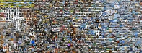
Figure 2. ImageNet dataset
Some recent studies have shown that, after a CNN is trained on the datasets for image classification tasks, the eigenvectors outputted from the intermediate layers can be used to complete other tasks excellently. In addition, our CNN is a VGG network, which performs exceptionally in transfer learning. To sum up, this paper firstly pretrains the CNN with ImageNet, a task-independent task, to generate the initial model. Next, the initial model was finetuned with a small dataset of book page images, such that the knowledge domain of the CNN transfers from image classification to book page retrieval.
As shown in Figure 2, the ImageNet dataset contains a total of 1.2 million images in 1,000 classes. The images are disturbed by geometric distortion, perspective variation, and scale difference.
Moreover, this paper chooses Softmax as the loss function of the pretained model. The Softmax loss function applies to the training of multi-class classifiers. The function can be expressed as:
SoftmaxLoss $=-\log P_{k}$ (1)
where, k∈{,1...,K} is the class label; Pk is the probability density:
$P_{k}=\frac{e^{x_{k}}}{\sum_{j=1}^{K} e^{x_{j}}}$ (2)
The meaning of Pk is the probability for a normalized data sample x to belong to class k. The above formulas show that the loss function can converge to the minimum, if each sample is assigned the class label with the highest probability. This is in line with the training objective of CNN.
The CNN pretrained on ImageNet has fully learned the representation of image features. The next task is to transfer the knowledge domain of the CNN from image classification to book page retrieval. To this end, the network was finetuned with a small dataset of book page images to further consolidate and optimize CNN parameters, making the network more suitable for the retrieval of book page images.
3.1 Dataset preparation
To optimize the CNN, this paper collects 8,000 book pages, and scans them in turn to obtain candidate standard images on book pages. After that, five different images were shot on each book page by a smart camera. These images were taken as the book page images to be tested. Note that the actual conditions were fully considered during the shooting. Thus, the images to be tested cover various disturbances, such as background clutter, local highlights, geometric deformation, perspective variation, and scale difference.
Through the above process, the authors obtained a dataset containing 8,000 candidate standard images, and 36,000 book page images to be detected. From the candidate standard images, 4,000 standard images were randomly selected. These images, along with the corresponding 16,000 images to be tested, were utilized to finetune the CNN.
Firstly, each of 16,000 the book page images were preprocessed to eliminate the influence of background clutter and geometric deformation, turning the image size to 224×224. Next, each preprocessed image to be tested was coupled with the corresponding candidate standard image into a standard sample pair, and with another randomly selected candidate standard image into a non-standard sample pair. In this way, 36,000 image pairs were ready for finetuning the CNN. Half of these images are standard samples, and half are non-standard samples. Furthermore, 24,000 sample pairs were selected as the training samples for the model. The rest 10,000 sample pairs were used to test the training effect. Figure 3 shows the entire dataset.
Figure 3. Dataset for network finetuning
3.2 Dataset optimization
The CNN pretrained on ImageNet intends to complete image classification. To transfer the knowledge domain of the CNN from image classification to book page retrieval, this paper finetunes the pretrained CNN with a small dataset of book page images. The training structure is the Siamese network, the earliest training network for face recognition models. The objective function of the network uses contrastive loss.
The Siamese network, coupled from two identical CNNs through parameter sharing, receives image pairs, and aims to gradually reduce the distance between positive sample pairs, and widen the distance between negative sample pairs. After network training, the two CNNs making up the network will have the same network parameters. Each CNN can independently express and extract image features. This training mode increases the similarity between each image to be tested and the corresponding standard image, and reduces that between each image to be tested and another image. This is conducive to the subsequent similarity calculation, and matching accuracy. The contrastive loss function can be expressed as:
ContrastiveLoss $=\|p-q\|_{2}^{2}$
$p, q$ is a positive sample pair
ContrastiveLoss $=\max \left(0, m-\|p-q\|_{2}^{2}\right)$
$p, q$ is a negative sample pair (3)
where, p, q is a pair of input images; m is the control factor regulating the lower bound of the interval between positive sample and negative sample pairs. According to the objective function, as the loss function approaches the minimum through the training, the distance between positive sample pairs will gradually reduce to zero, while that between negative sample pairs will gradually widen. Then, the lower bound of the interval between positive sample and negative sample pairs gradually approximates m.
Figure 4. Basic structure of our Siamese network
Table 2. Training parameters for network finetuning
|
Training parameter |
Value |
|
base_lr:# basic learning rate |
0.0001 |
|
momentum:# momentum factor |
0.9 |
|
weight_decay:# learning rate attenuation factor |
0.00005 |
|
test_interval:# number of iterations for each attenuation |
1000 |
|
max_iter:# maximum number of iterations |
60000 |
|
Solver_mode:#CPU or GPU |
GPU |
Overall, our finetuning network is a Siamese network composed of two CNNs, with contrastive loss as the loss function. The general structure of the network is illustrated in Figure 4.
Since the CNN has been pretrained, the initial learning rate was set to a low level for finetuning. By gradient descent with moment, the learning rate was attenuated after each specified number of iterations. The optimal network was determined by slowing down network convergence. Table 2 lists the relevant training parameters.
After finetuning, any single CNN can complete feature extraction of book page images, for the two CNNs of Siamese share the same network parameters. During the extraction of book page image features, the eigenvector outputted by a fully-connected layer was employed as the feature representation of the corresponding book page image. Contrastive experiments show that the eigenvalue from the fully-connected layer F6 of the CNN led to the best retrieval results. Therefore, this paper adopts the 4,096-dimensional single-precision eigenvector outputted by the F6 layer of the CNN as the feature representation of the corresponding image.
The proposed method was tested and verified through experiments on five aspects:
(1) Performance of direct retrieval of image features;
(2) Necessity of image segmentation and geometric correction;
(3) Necessity of CNN finetuning;
(4) Comparison between the effect of using each of the eigenvector outputted by the three fully-connected layers in the CNN;
(5) Redundancy of image features.
4.1 Experimental setup
(1) Dataset and data library
Our test set includes the 25,000 book page images to be tested, which are not used to finetuning in Section 3.2. The data library for our experiments has two image sources: 10,000 standard book page images were obtained by scanning in that section; 100,000 standard book page images were acquired from the Internet. The two parts were combined to obtain a data library of 150,000 candidate book page images.
(2) Performance metric
The performance of book page retrieval was evaluated by the top-k hit rate:
$\gamma_{k}=\frac{N_{k}}{N}$ (4)
where, N is the number of book page retrieval tests; Nk is the number of successful tests. A test is considered as successful, when the standard image corresponding to the image to be tested in contained in the top-k most similar candidate standard images.
4.2 Results analysis
(1) Performance of direct retrieval of image features
To verify its performance, our method was adopted to extract the features of the book page images to be tested. Then, the output 4,096-dimensional vector was not compressed, but directly used to feature matching with the eigenvectors of the candidate standard images in the data library. The top-k hit rates on the test set were counted. The Euclidean distance was adopted to measure the similarity in the test. In addition, our method was compared with a state-of-art end-to-end image retrieval method.
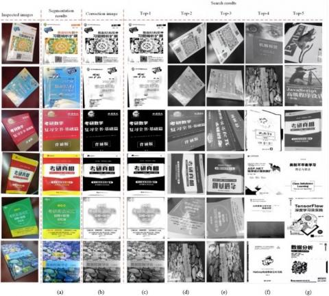
Figure 5 shows some typical retrieval results of our method. The correct candidate standard images are marked in green. Comparing Figures 5(a) and 5(b), it can be seen that our method can accurately distinguish between highly similar images of children's book pages. As shown in Figure 5(c), our method was robust in differentiating between children's book pages that are fuzzy or locally highlighted. It can be seen from Figures 5(d) and 5(e) that, our method could obtain accurate retrieval results, when the images were segmented by complex backgrounds or unsatisfactorily correctly geometrically. Figures 5(f) and 5(g) demonstrate the ability of our method to retrieve rotated images satisfactorily. Overall, our method has a high robustness on real-world disturbances such as fuzziness, local highlights, complex backgrounds, geometric deformation, and rotation. It always achieved outstanding retrieval results, despite these disturbances.
Figure 5. Retrieval results of our experiments
Table 3. Typical retrieval results of our method
|
Method |
Hit rate (%) |
||||
|
Top-1 |
Top-2 |
Top-3 |
Top-4 |
Top-5 |
|
|
LeCun’s method [17] |
17.13 |
24.41 |
37.15 |
48.33 |
53.19 |
|
Our method |
92.82 |
93.17 |
93.91 |
94.14 |
94.68 |
Table 3 compares the hit rates of our method with those of the CNN-based image retrieval method in LeCun’s work [17]. The contrastive method is the most advanced end-to-end CNN-based strategy for image retrieval. For fairness, both our method and the contrastive method were pretrained on the ImageNet dataset, and finetuned on the same book page dataset. The results show that the Top-5 hit rate of our method was as high as 94.68%, while that of the contrastive method was only 53.19%. Hence, our method can retrieve book page images more accurately than the state-of-the-art, without feature compression. In addition, the results of the contrastive method indicate the difficulty in retrieving book page images ideally by directly applying the CNN after pretraining and finetuning. This indirectly shows the necessity of our image preprocessing to book page retrieval.
(2) Necessity of image segmentation and geometric correction
Table 4 displays the hit rates of book page retrieval using our method, our method without geometric correction, and our method without both geometric correction and image segmentation. The results show that, after geometric correction and image segmentation, our method had a Top-5 hit rate of 94.68%; without geometric correction, the hit rate dropped to 57.23%; without geometric correction and image segmentation, the rate further declined to 54.58%. Therefore, both geometric correction and image segmentation are necessary steps for book page retrieval.
Table 4. Hit rates of our method without image segmentation and geometric correction (%)
|
Method |
Hit rate (%) |
||||
|
Top-1 |
Top-2 |
Top-3 |
Top-4 |
Top-5 |
|
|
With image segmentation and geometric correction |
92.82 |
93.17 |
93.91 |
94.14 |
94.68 |
|
Without geometric correction |
20.14 |
30.33 |
42.62 |
51.11 |
57.23 |
|
Without image segmentation and geometric correction |
19.61 |
25.47 |
39.46 |
49.41 |
54.58 |
(3) Necessity of CNN finetuning
To demonstrate the necessity of CNN finetuning, the authors further compared the book page retrieval effects of the pretrained CNN and the pretrained and finetuned CNN. The similarity was still measured by Euclidean distance. The results are shown in Table 5.
As shown in Table 5, the finetuning improved the hit rates of book page retrieval. The Top-1 to Top-5 hit rates of pretrained and finetuned CNN were 1.81%, 1.51%, 1.12%, 0.79%, and 0.63% higher than those of the model only pretrained on a task-independent dataset, respectively. Hence, it is necessary to finetune the CNN pretrained on the task-independent dataset, using book page images. The finetuning can to a certain extent improve the retrieval of book pages.
Table 5. Hit rates before and after finetuning
|
Method |
Hit rate (%) |
||||
|
Top-1 |
Top-2 |
Top-3 |
Top-4 |
Top-5 |
|
|
Pretrained CNN |
90.95 |
91.63 |
92.54 |
93.21 |
93.93 |
|
Pretrained and finetuned CNN |
92.76 |
93.14 |
93.66 |
94.00 |
94.56 |
(4) Comparison between the effect of using each of the eigenvector outputted by the three fully-connected layers
Table 6 displays the hit rates of using each of the eigenvector outputted by the three fully-connected layers in the trained CNN. The eigenvectors outputted by F6 and F7 are 4,096-dimensional, and the eigenvector outputted by F8 is 1,000-dimensional. The results show that the best effect was achieved with the eigenvector outputted by F6 as the image feature. The retrieval accuracy declined, when the eigenvector outputted by F8 was taken as the image feature, because the dimensionality dropped to less than 1/4 of that of F6. Hence, the best feature representation can be realized by adopting the 4,096-dimensional eigenvector from F6 as the image feature.
Table 6. Comparison of hit rates of using each of the eigenvector outputted by the three fully-connected layers
|
Fully-connected layer |
Hit rate (%) |
||||
|
Top-1 |
Top-2 |
Top-3 |
Top-4 |
Top-5 |
|
|
F6 |
92.38 |
93.15 |
93.93 |
94.21 |
94.57 |
|
F7 |
91.11 |
91.75 |
92.3 |
92.34 |
93.99 |
|
F8 |
84.69 |
88.58 |
89.66 |
89.75 |
90.18 |
(5) Redundancy of image features
The 4,096-dimensional eigenvector was subjected to principal component analysis (PCA) to different degrees. The retrieval results were recorded under each condition, and discussed to reveal the redundancy of image features.
The PCA was performed on the book page images to be tested and the candidate standard images in the data library, and the Top-k hit rates were recorded at different compression degrees. The feature compression of the PCA is described as follows:
Let X denote the 4,096-dimensional eigenvector, and m denote the scale of the standard images in the data library. Then, the eigenvectors of all candidate images constitute a 4,096×m-dimensional matrix M.
Step 1. For each row of the matrix, subtract the mean eigenvalue of that row from the eigenvalue of each row, and decentralize the result to obtain matrix M’.
Step 2. Compute the variance matrix 2 of matrix M’.
Step 3. Solve the eigenvector matrix U = SVD (M’’) through singular value decomposition (SVD).
Step 4. Screen the first d columns of U to form the compression matrix Ua.
Step 5. Compress any 4,096-dimensional eigenvector X to d dimensions:
$d=\frac{\gamma_{k}}{N}$ (5)
where, $\gamma_{k}$ is the compressed image feature; d is the dimensionality of the compressed feature.
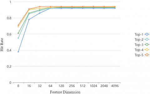
Figure 6 shows the variation in Top-k hit rates after the 4,096-dimensional eigenvector undergoes different degrees of PCA. The ordinate is the hit rates, where the Top-1 to Top-5 results are shown in broken lines of different colors; the abscissa is the feature dimensionality after PCA. It can be seen that the book page retrieval accuracy was not significantly affected, as the 4,096-dimensional eigenvector was reduced to 64 dimensions. However, the accuracy would drop obviously, once the dimensionality fell below 64. This means most feature information in the 4,096-dimensional image feature obtained by our CNN are redundant. The key useful information only takes up a very small portion.
Figure 6. Influence of compressed dimensionality on the hit rates of book page retrieval
The following conclusions were drawn through our experiments:
(1) In our method, the image features extracted by the CNN is directly applied to book page retrieval. The retrieval effect is quite satisfactory. The exceptionally good performance of our method was demonstrated in contrast to a representative method.
(2) Without geometric correction and image segmentation, the accuracy of our method in book page retrieval declined drastically. Therefore, both geometric correction and image segmentation are necessary steps for book page retrieval.
(3) The retrieval accuracy of the pretrained and finetuned CNN was higher than that of the model only pretrained on a task-independent dataset, indicating that the former is more suitable for our task of book page retrieval.
(4) The eigenvector outputted by F6, F7, and F8 of our CNN was adopted as the image feature representation in turn. The experimental results show that the best effect was achieved by F6, followed by F7, and the worst was achieved by F8. Hence, the eigenvector outputted by F6 should be chosen to represent image features.
(5) The PCA was performed on the 4,096-dimensional eigenvector. The accuracy of book page retrieval did not significantly worsen, when the compressed dimensionality was equal to or greater than 64. This means most feature information in the 4,096-dimensional image feature obtained by our CNN are redundant. The key useful information only takes up a very small portion. In actual retrieval tasks, the redundant information will greatly push up the computing overhead in feature matching. The efficiency of book page retrieval will be low, if the image features are directly adopted. It is necessary to further optimize the features to speed up the computing, and improve the retrieval efficiency.
[1] Liu, L., Zhao, Y., Zhou, H., Chen, J. (2017). Book page identification using convolutional neural networks trained by task-unrelated dataset. In International Conference on Image and Graphics, Shanghai, China, pp. 651-663. https://doi.org/10.1007/978-3-319-71607-7_57
[2] Babenko, A., Slesarev, A., Chigorin, A., Lempitsky, V. (2014). Neural codes for image retrieval. In European Conference on Computer Vision, Zurich, Switzerland, pp. 584-599. https://doi.org/10.1007/978-3-319-10590-1_38
[3] Kulis, B., Darrell, T. (2009). Learning to hash with binary reconstructive embeddings. NIPS'09: Proceedings of the 22nd International Conference on Neural Information Processing Systems, Vancouver British Columbia, Canada, pp. 1042-1050.
[4] Liu, W., Wang, J., Kumar, S., Chang, S.F. (2011). Hashing with graphs. In Proceedings of the 28th International Conference on Machine Learning, Bellevue, WA, USA, pp. 1-8.
[5] Eva, O.D., Lazar, A.M. (2019). Amplitude modulation index as feature in a brain computer interface. Traitement du Signal, 36(3): 201-207. https://doi.org/10.18280/ts.360301
[6] Gong, Y., Lazebnik, S., Gordo, A., Perronnin, F. (2012). Iterative quantization: A procrustean approach to learning binary codes for large-scale image retrieval. IEEE Transactions on Pattern Analysis and Machine Intelligence, 35(12): 2916-2929. https://doi.org/10.1109/TPAMI.2012.193
[7] Liu, H., Wang, R., Shan, S., Chen, X. (2016). Deep supervised hashing for fast image retrieval. In Proceedings of the IEEE Conference on Computer Vision and Pattern Recognition, Vegas, NV, USA, pp. 2064-2072. https://doi.org/10.1109/CVPR.2016.227
[8] Li, W.J., Wang, S., Kang, W.C. (2016). Feature learning based deep supervised hashing with pairwise labels. IJCAI'16: Proceedings of the Twenty-Fifth International Joint Conference on Artificial Intelligence, New York USA, pp. 1711-1717.
[9] Yang, H.F., Lin, K., Chen, C.S. (2017). Supervised learning of semantics-preserving hash via deep convolutional neural networks. IEEE Transactions on Pattern Analysis and Machine Intelligence, 40(2): 437-451. https://doi.org/10.1109/TPAMI.2017.2666812
[10] Liu, L., Shen, F., Shen, Y., Liu, X., Shao, L. (2017). Deep sketch hashing: Fast free-hand sketch-based image retrieval. In 2017 IEEE Conference on Computer Vision and Pattern Recognition (CVPR), Honolulu, HI, USA, pp. 2862-2871. https://doi.org/10.1109/CVPR.2017.247
[11] Cao, Z., Long, M., Wang, J., Yu, P.S. (2017). Hashnet: Deep learning to hash by continuation. In 2017 IEEE International Conference on Computer Vision (ICCV), Venice, Italy, pp. 5608-5617. https://doi.org/10.1109/ICCV.2017.598
[12] Cao, Y., Long, M., Wang, J., Liu, S. (2017). Deep visual-semantic quantization for efficient image retrieval. In Proceedings of the IEEE Conference on Computer Vision and Pattern Recognition, Honolulu, HI, USA, pp. 1328-1337. https://doi.org/10.1109/CVPR.2017.104
[13] Cao, Y., Long, M., Liu, B., Wang, J. (2018). Deep Cauchy hashing for hamming space retrieval. In Proceedings of the IEEE Conference on Computer Vision and Pattern Recognition, Lake City, UT, USA, pp. 1229-1237. https://doi.org/10.1109/CVPR.2018.00134
[14] Boykov, Y.Y., Jolly, M.P. (2001). Interactive graph cuts for optimal boundary & region segmentation of objects in ND images. In Proceedings Eighth IEEE International Conference on Computer Vision, ICCV 2001, Vancouver, BC, Canada, pp. 105-112. https://doi.org/10.1109/ICCV.2001.937505
[15] Rother, C., Kolmogorov, V., Blake, A. (2004). "GrabCut" interactive foreground extraction using iterated graph cuts. ACM Transactions on Graphics (TOG), 23(3): 309-314. https://doi.org/10.1145/1015706.1015720
[16] Cheng, M.M., Prisacariu, V.A., Zheng, S., Torr, P.H., Rother, C. (2015, October). DenseCut: Densely connected CRFs for realtime GrabCut. In Computer Graphics Forum, 34(7): 193-201. https://doi.org/10.1111/cgf.12758
[17] Deng, J., Dong, W., Socher, R., Li, L.J., Li, K., Li, F.F. (2009). Imagenet: A large-scale hierarchical image database. In 2009 IEEE Conference on Computer Vision and Pattern Recognition, pp. 248-255. https://doi.org/10.1109/CVPR.2009.5206848
[18] LeCun, Y., Bottou, L., Bengio, Y., Haffner, P. (1998). Gradient-based learning applied to document recognition. Proceedings of the IEEE, 86(11): 2278-2324. https://doi.org/10.1109/5.726791
[19] He, K., Zhang, X., Ren, S., Sun, J. (2016). Deep residual learning for image recognition. In 2016 IEEE Conference on Computer Vision and Pattern Recognition (CVPR), Las Vegas, NV, USA, pp. 770-778. https://doi.org/10.1109/CVPR.2016.90
[20] Sainuddin, S., Subali, B., Jailani, Elvira, M. (2022). The development and validation prospective mathematics teachers holistic assessment tools. Ingénierie des Systèmes d’Informatio, 27(2): 171-184. https://doi.org/10.18280/isi.270201
[21] Amanzadeh, S., Forghani, Y., Chabok, J.M. (2020). Improvements on learning kernel extended dictionary for face recognition. Revue d'Intelligence Artificielle, 34(4): 387-394. https://doi.org/10.18280/ria.340402