Zhi Cui* | Zhenhua Cai
© 2022 IIETA. This article is published by IIETA and is licensed under the CC BY 4.0 license (http://creativecommons.org/licenses/by/4.0/).
OPEN ACCESS
During the feature extraction of hyperspectral images, a single filter cannot acquire complete information. To solve the problem, this paper proposes a feature extraction method based on subspace band selection and transform-domain recursive filtering. The proposed method contains three steps: Firstly, the target hyperspectral image is divided into multiple subsets of adjacent bands. Secondly, the Lasso-based band selection approach is adopted to compute the sparsity coefficient of each band. The bands in each subset are then ranked by the coefficient. Based on the ranking, the band with the highest coefficient is extracted from each subset, and used to reconstruct the hyperspectral data. Finally, the reconstructed hyperspectral image is processed through transform-domain recursive filtering, producing the features to be classified. Taking the support vector machine (SVM) as the classifier, our method was tested on several real hyperspectral image datasets. The results show that our method has a better classification accuracy than the other band selection methods.
feature extraction, hyperspectral image, subspace band selection, transform-domain recursive filtering
Hyperspectral remoting sensing can provide researchers with hyperspectral images, and uniquely differentiate between different land covers by fine spectral features. Thanks to this huge advantage, hyperspectral remoting sensing has been extensively applied to target detection, urban planning, modern agriculture, and environmental monitoring [1].
In a hyperspectral image, each pixel corresponds to a spectral curve that reflects the inherent physical, chemical, and optical properties of the ground material. Different kinds of images can be obtained by labeling the pixels of different ground materials based on the unique features of each pixel. This strategy is called hyperspectral image classification.
General image classification methods aim to identify the primary and secondary contents in the scene. By contrast, hyperspectral image classification intends to assign a unique class label to each pixel in the hyperspectral image. Many effective methods have been developed to realize this goal, such as Bayesian estimation [2], support vector machine (SVM) [3], and sparse representation [4]. When only a few samples are labeled, however, most of these classifiers cannot achieve satisfactory classification performance, owing to the curse of dimensionality. In addition, the adjacent noiseless hyperspectral bands are usually closely correlated with each other. The high spectral dimensions mean a rise in the computing load of the classification process.
Dimension reduction can effectively reduce the number of bands. The traditional approach of dimension reduction loads all samples and all bands to the memory, which is not suitable for handling the massive data in the big data environment. Facing such a complex scene, it is challenging to remove redundant and unrelated information in a reasonable time.
Feature extraction and feature selection are two common spectral dimension reduction methods in hyperspectral image processing. The general step of feature extraction is to map the hyperspectral image to another feature space through linear transformation, and retain the important components of the image according to the transformed coefficient size, laying the basis for image classification. The mainstream feature extraction methods include principal component analysis (PCA) [5], independent component analysis (ICA) [6], and linear discriminant analysis (LDA) [7]. The PCA preserves most information of the hyperspectral image in a few significant principal components, but the few preserved components are spectral features that interest people. The ICA calculates highly independent transformation components. Yet this strategy is so complex as to bring a heavy computing load. Moreover, the above feature extraction methods only use the spectral information of hyperspectral images, failing to consider the spatial continuity of hyperspectral images. This clearly affects the calculation effect.
Feature selection aims to find the most representative data subset in the hyperspectral image, and use the selected subset to complete the final task of image classification. Well-known feature selection methods are distance-based method [8], information-based method [9], and band selection method [10].
To simultaneously utilize the spectral and space information in the hyperspectral image, researchers have recently presented the hyperspectral image classification method based on the combination between spectral and spatial features, namely, the watershed method [11], minimum spanning tree [12], hierarchical segmentation [13], and partition clustering [14]. These methods fully consider the spatially continuous information in the hyperspectral image, i.e., the strong correlation between adjacent pixels, and introduce the spatial correlation to image classification, thereby achieving a high classification accuracy. However, they depend largely on the automatic segmentation or prior optimization of the hyperspectral image, and consume much time.
In recent years, edge-preserving filters become a hot topic in hyperspectral image processing, owing to their superiority in keeping image edge features. These filters have been widely adopted for highly dynamic imaging, three-dimensional (3D) matching, and image fusion [15]. This paper introduces the transform-domain recursive filter, an edge-preserving filter, to hyperspectral image classification, and proposes a classification method based on subspace band selection and transform-domain recursive filtering (BSTDRF). Firstly, the original hyperspectral image was divided into multiple subsets of adjacent bands. Next, the Lasso-based band selection approach was adopted to extract the bands with the largest sparsity coefficient and the highest representativeness, which were used to reconstruct the new hyperspectral image data. Thirdly, the reconstructed hyperspectral image was processed through transform-domain recursive filtering, producing suitable features. Finally, the image classification was completed, with SVM as the classifier.
Our method is based on two hypotheses: Firstly, the adjacent bands in the hyperspectral image data contain redundant information. Secondly, there is a strong correlation between adjacent pixels in the hyperspectral image. For the first hypothesis, the band selection was completed by choosing several most suitable bands from the set of all bands in the hyperspectral image data, and using them to construct the new hyperspectral image data. The physical meaning of the spectral bands can be preserved well, and the redundant information can be largely removed, because new features do not need to be obtained through linear or nonlinear transform. For the second hypothesis, the transform-domain recursive filtering can ensure that the adjacent pixels, whose edges belong to the same side of the image, have similar eigenvalues. Then, the spatial information of the hyperspectral image can be fully utilized for feature extraction. Experimental results show that our BSTDRF method improves the classification accuracy of hyperspectral images.
The remainder of this paper is organized as follows: Section 2 introduces the basic theories; Section 3 describes the proposed BSTDRF method; Section 4 presents the experimental results; Section 5 puts forward the research conclusions.
2.1 Lasso-based band selection
For hyperspectral image data, there is a closer correlation between adjacent bands than non-adjacent bands. Thus, it is entirely feasible to sort the bands of a hyperspectral image using the Lasso algorithm. The steps of the algorithm are as follows:
For a hyperspectral image containing l types of land covers and N spectral bands, M training samples are given. Each sample has a known spectral type and sample label. Then, each pair of samples can be expressed as (xi, yi), where i \in[1,2, \cdots, N]. Sample xi is an M-dimensional column vector of the spectral response of the i-th sample. Obviously, the j-th element of xi is the spectral response of the j-th band of the hyperspectral image; yi is an l-dimensional column vector, representing the class labels of all i samples.
The Lasso algorithm introduces the l1 norm as a penalty term to the ordinary least squares (OLS) estimation, and ensures the sparsity of the solution of the linear regression problem. Then, the sparsity coefficient of each band can be obtained by:
$\hat{\alpha}=\underset{\alpha}{\arg \min } \sum_{i=1}^{N} \frac{1}{2}\left\|\boldsymbol{y}_{i}-\alpha^{T} \boldsymbol{x}_{i}\right\|_{2}^{2}+\lambda\|\alpha\|_{1}$ (1)
where, yi is the class label of a sample; coefficient α is an N+1-dimensional column vector; N is the dimensions of the original hyperspectral image (i.e., the number of bands).
Since the norm is singular on the vertex of each orthonormal basis, the coefficient α calculated by formula (1) is sparse. λ is the regularization parameter used to adjust the sparsity of the solution.
2.2 Transform-domain recursive filtering
Transform-domain recursive filtering is an edge-preserving filter. It is capable of preserving the edges, lines and other details of the image, while smoothing the texture and noise in the image. Thanks to this advantage, the transform-domain filter and other edge-preserving filters have piqued much interest among researchers in the field of image processing. For example, Wang et al. [16] used edge-preserving filters to extract features from hyperspectral images, and fully utilized the spectral information and spatial information of the image in the post-processing of pixel-based classification results. Luo et al. [17] proposed a spectral-spatial feature extraction method based on edge-preserving filtering. The method removes unimportant parts of hyperspectral images, and further improves the interpretability of hyperspectral image classification results. Zhu et al. [18] decomposes the hyperspectral image through independent component analysis (ICA), and performs edge-preserving filtering on image edges, in order to extract the features for image classification.
This section only briefly describes the transform-domain recursive filter. The complete description is available in Gastal’s work [19].
Suppose there is a one-dimensional (1D) input signal I. Following the approximate distance-preserving transformation method, the input signal can be transformed to the transform domain Φ:
$\boldsymbol{V}_{i}=\boldsymbol{I}_{0}+\sum_{k=1}^{i}\left(1+\frac{\sigma_{s}}{\sigma_{r}}\left|\boldsymbol{I}_{j}-\boldsymbol{I}_{j-1}\right|\right)$ (2)
where, Vi, originally a function of distance calculation, is the transform domain signal; σs is the standard deviation of the spatial domain, responsible for adjusting the window size of the filter; σr is the standard deviation of the value domain, responsible for adjusting the fuzziness of the filter. Then, the input signal I is subject to recursive filtering:
$\boldsymbol{W}_{i}=\left(1-\omega^{\rho}\right) \boldsymbol{I}_{i}+\omega^{\rho} \boldsymbol{W}_{i-1}$ (3)
where, Wi is the filter output for the i-th pixel in the input signal I; $\rho=\exp \left(-\frac{\sqrt{2}}{\sigma_{s}}\right)$, $\rho \in[0,1]$ is a feedback signal; ω is a distance coefficient representing the distance between two adjacent pixels Wi and Wi-1 in the transform domain. Obviously, as the feedback signal increases, ωρ will gradually decrease until reaching zero. Then, the propagation chain will be stopped, and the edges of the signal will be preserved.
For two-dimensional (2D) images, transform-domain recursive filter processes the image by performing 1D operations along each dimension of the image. Sun and Du [20] demonstrated that the iterative execution of three 1D filtering operations can obtain filtered images without artifacts.
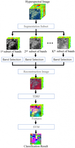
As shown in Figure 1, the proposed hyperspectral image feature extraction method, which is based on subspace band selection and transform-domain recursive filtering, includes the following five steps:
(1) Divide the hyperspectral image into multiple subsets of adjacent bands.
(2) For the adjacent bands in each subset, use the Lasso-based band selection method to calculate their coefficients, and sort the coefficients.
(3) According to the sorting results, select the bands with large coefficients in each subset to form a new hyperspectral image.
(4) Perform a transform-domain recursive filtering on the reconstructed new hyperspectral image to obtain the features to be classified.
(5) Input the features obtained in the previous step into the SVM classifier to obtain the final classification result.
(1) Band partition
In this step, the hyperspectral image is partitioned into several equal-sized subsets by the simple bisection method. Specifically, the given N-dimensional hyperspectral data P is decomposed into K equal-sized subsets of hyperspectral bands, N/K, $P=P_{1}, P_{2}, \cdots P_{K}$. Note that, if N/K is not divisible, the k-th subset $(k=1,2,3, \cdots, K)$ can be represented by:
$\mathbf{P}_{k}=\lfloor N / K\rfloor+K(N / K-\lfloor N / K\rfloor)$ (4)
where, $\lfloor N / K\rfloor$ is the largest integer less than or equal to N/K; K is the number of subsets of hyperspectral bands.
(2) Feature selection
After dividing the hyperspectral band subsets, the Lasso-based band selection is performed on each subset. The coefficient of each band is solved by formula (1) and sorted in descending order.
(3) Hyperspectral data reconstruction
To reconstruct the hyperspectral data, according to the sorting results in Step (2), the band with the highest coefficient and ranking is chosen from each subset of hyperspectral bands by:
$\mathbf{P}_{r e c}=\sum_{i=1}^{K} \sum_{n=1}^{K} \mathbf{P}_{n}^{i}$ (5)
where, $P_{\text {rec }}$ is the reconstructed hyperspectral data; K is the number of subsets of hyperspectral bands, where the k-th subset is denoted by $k \in(1, K)$; $P_{n}^{i}$ is the i-th ranking band in the n-th subset of hyperspectral bands.
Only the top-ranking band (the one with the highest coefficient) is selected from each subset. On this basis, a hyperspectral data containing K bands can be reconstructed by formula (5). Note that the maximum ranking must be smaller than or equal to K. If the top-k bands are selected from each subset, the reconstructed hyperspectral data would contain k•K bands.
(4) Transform-domain recursive filtering
After reconstructing the hyperspectral image, the reconstructed data is subjected to transform-domain recursive filtering to obtain the features F to be classified:
$\boldsymbol{F}=\operatorname{TDRF}\left(\boldsymbol{I}, \sigma_{s}, \sigma_{r}\right)$ (6)
where, I is the reconstructed data of the hyperspectral image; σs and σr are parameters adjusting the filter smoothness.
(5) Classification
The proposed BSTDRF method extracts features from the hyperspectral image data. Subsequently, the data classification is performed by other professional classifiers. The SVM is a popular pixel classifier with superior performance in classification accuracy. Besides, the classifier is not sensitive to the dimensionality of hyperspectral data. Given these advantages, this paper takes the SVM to classify the reconstructed hyperspectral data.
Figure 1. Schematic of the proposed BSTDRF classification method
4.1 Experimental setup
(1) Datasets
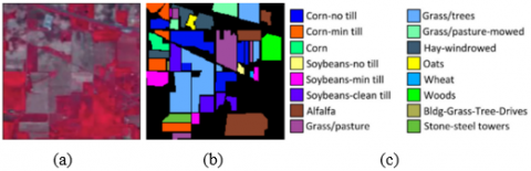
To verify the classification performance of BSTDRF on hyperspectral images, two real hyperspectral datasets were adopted for experiments: the Indian Pines dataset (Figure 2) and the University of Pavia dataset (Figure 3).
Figure 2. Indian Pine dataset (a) Pseudo-color image of the Indian Pines image, (b) Reference data, (c) Class names
Figure 3. University of Pavia dataset (a) Pseudo-color image of the University of Pavia image, (b) Reference data, (c) Class names
In 1992, the Indian Pines image was taken by an airborne visible infra-red imaging spectrometer (AVIRIS) in the Indian Pines lab base in northwestern Indiana, United States. This remote sensing image (size: 145 × 145 × 22) has a spatial resolution of 20m, and a wavelength range of 0.4-2.5μm. Before the hyperspectral image classification experiment, the spectral bands covering water absorbing areas must be removed from the original hyperspectral data: [104-108], [150-163], and 220. The removal reduced the number of spectral bands from 220 to 200.
The Indian Pines image contains multiple native vegetation, including farmland, forest, and others. According to the current exploration, the scene can be divided into 16 different targets: Class 1 represents Alfalfa, Class 2 represents Corn-no till, Class 3 represents Corn-min till, Class 4 represents Corn, Class 5 represents Grass/pasture, Class 6 represents Grass/trees, Class 7 represents Grass/pasture-moved, Class 8 represents Hay-windrowed, Class 9 represents Oats, Class 10 represents Soybeans-no till, Class 11 represents Soybeans-min till, Class 12 represents Soybeans-clean till, Class 13 represents Wheat, Class 14 represents Woods, Class 14 represents Buildings, and Class 16 represents Stone-steel towers.
The University of Pavia image was collected by a German reflective optics system imaging spectrometer from a city near the University of Pavia, Italy. This airborne image has a spatial resolution of 1.3m, and a wavelength range of 0.43-0.86μm. The 610 × 340 sized image contains 115 bands. Before the experiment, the 12 most noisy bands were removed.
There are nine different ground covers in the scene of University of Pavia: Asphalt (Class 1), Meadows (Class 2), Gravel (Class 3), Trees (Class 4), Metal sheets (Class 5), Soil (Class 6), Bitumen (Class 7), Bricks (Class 8), and Shadows (Class 9).
(2) Quality metrics
After classifying each hyperspectral image, it is necessary to evaluate the classification effect. The classification accuracy should be assessed against ground reference data. This paper adopts three common metrics of the classification accuracy of hyperspectral images, namely, overall accuracy (OA), average accuracy (AA), and Kappa coefficient. Among them, OA measures the percentage of pixels being classified correctly; AA refers to the mean percentage of correctly classified pixels in each class; Kappa coefficient excels in estimating the recognition accuracy, in the light of the impact of uncertainties on the classification results.
4.2 Classification results
(1) Parameter analysis
(a) Influence of σs
(b) Influence of σr
Figure 4. Analysis of the parameters σr and σs on Indian Pines data set
The proposed BSTDRF adopts the transform-domain recursive filtering technique. It is necessary to understand the roles of filter parameters σs and σr in classification, and determine their optimal values. That is why the Indian Pines image was selected for experiment.
During the experiment, 10% of samples from the Indian Pines dataset were chosen randomly as the training set, and the remaining 90% as the test set. Through cross validation, an empirical value was configured for σr. Different σs values were selected until the output was nearly optimal. Then, the σs value at the moment was recorded, and taken as the optimal filter parameter of BSTDRF. Next, the σs was fixed at the optimal value obtained in the first step, and different σr were selected until the output was nearly optimal. In this way, the two parameters of the transform-domain recursive filter were determined. The specific process is as follows:
Firstly, σr was fixed at 0.4, while σs was gradually increased from 10 to 100. The classification results are displayed in Figure 4(a). It can be learned that OA and AA reached the optimal level, when σs=70. After σs surpassed 70, OA, AA and Kappa coefficient all started to decline. This means an excessively large window of the filter will cause the loss of details. The spatial coefficient should be controlled within the effective range.
Secondly, σs was fixed at 70, while σr was gradually increased from 0.1 to 1.0. The classification results are displayed in Figure 4(b). It can be observed that all three indices fell on a low level, when σr was small. The undesired classification effect is attributable to the fact that a small filter parameter can only extract a limited number of features from a small neighborhood. When σr was large, all three metrics started to decrease. Thus, when the value domain parameter is large, the transform-domain recursive filter is approximately equivalent to a Gaussian filter, which makes the image fuzzy. When σr=0.4, the overall performance of the three parameters was the best. Overall, this paper sets σs as 70, and σr as 0.4.
(2) Comparison of different classification methods
Our BSTDRF was compared with seven widely used classifiers of hyperspectral images, namely, SVM, PCA-based SVM, ICA-based SVM, multidimensional scaling (MDS)-based SVM [21], extended morphological profiles (EMP) [22], linear regression for machine learning (LRML) [23], and DTB [24].
The SVM methods were realized using the LIBSVM library and the radial basis function (RBF) kernel. The parameters of each SVM classifier were determined through five-fold cross-validation. All experiments were conducted using MATLAB 2019 on a computer with Intel Core i7-8700 CPU and 16 GB RAM. To ensure the objectivity of the evaluation, each experiment was repeated 10 times with random training samples. For PCA and ICA, the top-20 principal or independent components were imported to the filter, and the default parameter setting was adopted for the remaining methods.
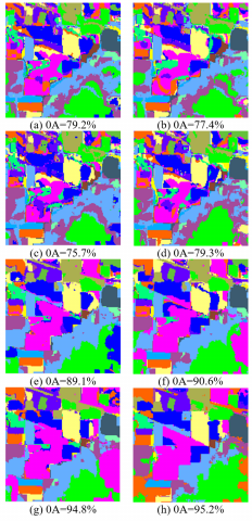
The first experiment was carried out on the Indian Pines dataset. 10% of the samples were randomly selected as training samples, and the remaining 90% were used as test samples. Figure 5 shows the classification results and OAs of different algorithms. It can be observed that the EMP achieved better classification accuracy (OA=89.1%) than pixel-level feature extraction algorithms, by utilizing the spatial structure information in the image. However, some noises remained in the classification results of EMP. LRML, DTB and BSTDRF all effectively removed the incorrect classification, which looks like noises, and achieved better recognition accuracy. Our BSTDRF achieved the best OA, which is 20.2% higher than that of SVM, 5.1% higher than that of LRML, and 0.4% higher than that of DTB. Hence, reconstructing the hyperspectral image with important bands can reduce the spectral dimensionality of the hyperspectral image, eliminate noisy bands, and retrain the useful information in the images.
Figure 5. Classification results obtained by different methods on Indian Pines dataset (a) SVM, (b) PCA-SVM, (c) ICA-SVM, (d) MDS-SVM, (e) EMP, (f) LRML, (g) DTB, (h) Proposed BSTDRF
Table 1 displays the OA, AA and Kappa coefficient of each method on each class in the scene. It can be seen that, when the training sample took up 10% of ground reference data, the SVM could effectively differentiate between ground targets with very different spectrums, such as Grass_M, Grass_T, Grass_P, Hay_W, Wheat, Woods, and Stone. However, this pixelwise classifier failed to recognize ground targets with similar spectrums, due to the neglection of the spatial information of the hyperspectral image. For instance, the classification accuracy on Corn was merely 43.7%, and that on Buildings was only 53.9%.
Compared with the classification directly on the original data of the hyperspectral image, PCA and ICA could effectively reduce the dimensionality of the data, but their OA declined by 2.3% - 4.6%.
EMP relies on the multiscale morphological operator to extract the spatial features from the hyperspectral image for classification. LRML introduces multilayer regression into the spatial information of the image, and optimizes the spectral classification result of logistics regression classifier. DTB introduces the spatial information of the image via multi-filter fusion, and thus optimizes the space of the spectral classification results. As shown in Table 1, these three spatial-spectral feature extractors outperformed the pixelwise classifier.
The proposed BSTDRF realized the highest OA, AA and Kappa coefficient. Compared with the original SVM, our approach improved the OA from 79.2% to 95.2%, the AA from 78.3% to 94.6%, and the Kappa coefficient from 76.9% to 95.4%. Some ground targets, namely, Buildings and Alfalfa, cannot be identified correctly by some pixelwise classifiers. Our approach can improve their classification accuracy to 91.5% and 81.3%, respectively.
The experiment on the Indian Pines scene suggests that our BSTDRF has better classification performance than other classification methods.
Table 1. Classification accuracies of different methods on the Indian Pines scene (10% for training set)
|
Class |
Train |
Test |
Different Classification Methods |
|||||||
|
SVM |
PCA-SVM |
ICA-SVM |
MDS-SVM |
EMP |
LRML |
DTB |
BSTDRF |
|||
|
1 |
23 |
23 |
65.4 |
62.8 |
61.9 |
64.6 |
87.2 |
89.3 |
94.5 |
94.7 |
|
2 |
79 |
1349 |
75.3 |
71.6 |
70.8 |
76.5 |
85.4 |
95.9 |
93.4 |
95.3 |
|
3 |
81 |
749 |
70.8 |
67.4 |
68.6 |
69.9 |
81.1 |
82.6 |
92.7 |
91.8 |
|
4 |
66 |
171 |
43.7 |
48.1 |
44.5 |
42.3 |
81.9 |
83.4 |
84.1 |
87.8 |
|
5 |
71 |
412 |
82.0 |
85.6 |
84.4 |
90.5 |
91.7 |
87.4 |
92.9 |
93.6 |
|
6 |
78 |
652 |
91.7 |
93.8 |
94.2 |
95.5 |
95.7 |
98.7 |
98.6 |
99.1 |
|
7 |
15 |
13 |
83.9 |
73.5 |
79.4 |
73.9 |
80.5 |
85.7 |
96.1 |
95.9 |
|
8 |
72 |
406 |
96.4 |
96.5 |
95.2 |
97.6 |
95.3 |
99.0 |
99.6 |
99.7 |
|
9 |
10 |
10 |
51.4 |
50.5 |
56.2 |
61.5 |
65.5 |
50.4 |
79.8 |
81.3 |
|
10 |
79 |
893 |
76.6 |
76.3 |
70.8 |
72.6 |
79.3 |
70.6 |
88.9 |
93.8 |
|
11 |
111 |
2344 |
85.1 |
84.4 |
83.5 |
83.7 |
91.4 |
92.3 |
97.6 |
98.7 |
|
12 |
74 |
519 |
79.0 |
74.2 |
77.4 |
73.9 |
81.9 |
89.1 |
93.2 |
95.1 |
|
13 |
64 |
141 |
91.9 |
93.6 |
91.7 |
97.0 |
97.6 |
99.9 |
89.3 |
90.9 |
|
14 |
84 |
1181 |
95.6 |
93.7 |
94.4 |
97.6 |
98.3 |
98.1 |
98.9 |
99.4 |
|
15 |
70 |
316 |
53.9 |
53.6 |
54.3 |
53.1 |
54.9 |
62.7 |
91.3 |
91.5 |
|
16 |
47 |
46 |
96.9 |
89.4 |
87.4 |
88.6 |
84.2 |
87.1 |
93.7 |
93.9 |
|
OA |
79.2 |
77.4 |
75.7 |
79.3 |
89.1 |
90.6 |
94.8 |
95.2 |
||
|
AA |
78.3 |
79.5 |
78.9 |
80.1 |
82.8 |
91.2 |
93.7 |
94.6 |
||
|
Kappa |
76.9 |
75.2 |
76.3 |
82.5 |
83.1 |
86.8 |
94.9 |
95.4 |
||
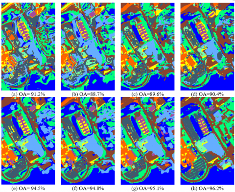
Figure 6. Classification results obtained by different methods on University of Pavia data set (a) SVM, (b) PCA-SVM, (c) ICA-SVM, (d) MDS-SVM, (e) EMP, (f) LRML, (g) DTB, (h) Proposed BSTDRF
Table 2. Classification accuracies of different methods on the University of Pavia scene (4% for training set)
|
Class |
Train |
Test |
Different Classification Methods |
|||||||
|
SVM |
PCA-SVM |
ICA-SVM |
MDS-SVM |
EMP |
LRML |
DTB |
BSTDRF |
|||
|
1 |
190 |
6641 |
94.1 |
92.5 |
91.1 |
90.8 |
93.7 |
96.5 |
97.3 |
97.7 |
|
2 |
191 |
18458 |
96.4 |
95.8 |
96.8 |
96.6 |
98.0 |
99.9 |
99.9 |
99.4 |
|
3 |
190 |
1909 |
69.3 |
67.9 |
65.8 |
68.3 |
69.5 |
70.1 |
75.4 |
78.1 |
|
4 |
190 |
2874 |
83.9 |
81.7 |
80.7 |
85.6 |
91.8 |
92.2 |
90.1 |
93.0 |
|
5 |
190 |
1155 |
97.2 |
97.6 |
97.3 |
98.8 |
99.3 |
99.2 |
99.8 |
99.9 |
|
6 |
190 |
4839 |
62.0 |
63.7 |
66.9 |
69.8 |
91.4 |
93.1 |
95.7 |
95.9 |
|
7 |
190 |
1140 |
72.3 |
74.1 |
79.2 |
80.4 |
92.7 |
93.8 |
93.5 |
94.3 |
|
8 |
190 |
3492 |
84.1 |
83.6 |
82.8 |
83.9 |
96.3 |
96.7 |
97.2 |
97.5 |
|
9 |
190 |
757 |
99.9 |
99.9 |
99.7 |
99.9 |
99.9 |
99.8 |
99.7 |
99.9 |
|
OA |
91.2 |
88.7 |
89.6 |
90.4 |
94.5 |
94.8 |
95.1 |
96.2 |
||
|
AA |
89.1 |
84.3 |
84.8 |
87.4 |
92.3 |
93.7 |
93.9 |
95.5 |
||
|
Kappa |
88.5 |
83.6 |
84.4 |
87.1 |
91.3 |
93.2 |
93.3 |
94.9 |
||
The second experiment was carried out on the University of Pavia dataset, which has many more ground references than Indian Pines dataset. Hence, 4% of samples were selected randomly for the training set, and the rest 96% for the test set. Figure 6 shows the classification results and OAs of different algorithms.
It can be seen that the four spatial-spectral classifiers, including EMP, LRML, DTB, and our approach, achieved better classification accuracy than the pixel-wise classification methods. In addition, the OA (96.2%) of our approach was better than that of the other three spatial-spectral classifiers. The advantage was 1.8% over EMP, 1.5% over LRML, and 1.2% over DTB. This is because our approach adopts the Lasso-based band selection strategy, which reduces the dimensionality of data, while preserving the physical meaning of the data.
Table 2 displays the OA, AA and Kappa coefficient of each method on each class in the University of Pavia scene. It can be seen that, among the four pixel-wise classifiers, the approach that directly imports the original data of hyperspectral images to the SVM, boasted the best effect. The other three pixel-wise methods, namely, PCA, ICA, and MDS, lost some useful information during dimensionality reduction, which affects the classification accuracy, although the dimensionality reduction improves calculation efficiency.
Taking the Gravel ground targets for example, the OA obtained after the dimensionality reduction by PCA, ICA, and MDS was 2.1%, 5.3%, and 1.5% lower than the OA achieved using the original data directly, respectively.
In addition, the pixel-wise classifiers fail to consider the spatial information of images, and thus performed poorly in recognizing some ground targets. For example, the highest OA of the pixel-wise classifiers was 69.8% (MDS), while the OA of our approach was 37.4% higher (95.9%).
The second experiment shows that our approach removes the noisy bands from the hyperspectral image through band selection, and retains the contours and edges of the image via transform-domain recursive filtering. Thus, our approach is suitable for precision agriculture, as well as urban planning.
This paper proposes a novel approach called BSTDRF for hyperspectral image classification. The proposed approach consists of two phases: data dimensionality reduction based on subspace band selection, and feature extraction based on transform-domain recursive filtering. Two experiments were carried out on real hyperspectral image datasets, namely, the agricultural scene of Indian Pines and the urban scene of University of Pavia. The results show that our approach achieved the best classification effect among all methods. Compared with the 7 contrastive methods, our BSTDRF has the following merits: Firstly, our approach can reduce the dimensionality of hyperspectral image data to the maximum possible degree, and remove the noisy bands as much as possible. Secondly, our approach can preserve the contours and edges of the original image, which contain the richest information in the image. However, our approach requires manual adjustment during the subspace segmentation of hyperspectral image data, and we only studied one edge-preserving filter: transform-domain recursive filtering. In future, we will further explore adaptive image segmentation techniques, and disclose the influence of different local filters on image segmentation accuracy.
This work is supported by the Scientific Research Fund of Hunan Provincial Education Department (Grant No.: 19B105).
[1] Liu, Y., Gao, G., Gu, Y. (2017). Tensor matched subspace detector for hyperspectral target detection. IEEE Transactions on Geoscience and Remote Sensing, 55(4): 1967-1974. https://doi.org/10.1109/tgrs.2016.2632863
[2] Bioucas-Dias, J., Plaza, A., Camps-Valls, G., Scheunders, P., Nasrabadi, N., Chanussot, J. (2013). Hyperspectral remote sensing data analysis and future challenges. IEEE Geoscience and Remote Sensing Magzine, 1(2): 6-36. https://doi.org/10.1109/mgrs.2013.2244672
[3] Wagle, S.A., R, H. (2021). Comparison of plant leaf classification using modified AlexNet and support vector machine. Traitement du Signal, 38(1): 79-87. https://doi.org/10.18280/ts.380108
[4] Dong, Y., Du, B., Zhang, L., Zhang, L. (2017). Dimensionality reduction and classification of hyperspectral images using ensemble discriminative local metric learning. IEEE Transactions on Geoscience and Remote Sensing, 55(5): 2509-2524. https://doi.org/10.1109/tgrs.2016.2645703
[5] Lu, T., Li, S., Fang, L., Bruzzone, L., Benediktsson, J. (2016). Set-to-set distance-based spectral-spatial classification of hyperspectral images. IEEE Transactions on Geoscience and Remote Sensing, 54(12): 7122-7134. https://doi.org/10.1109/tgrs.2016.2596260
[6] Kang, X., Li, S., Fang, L., Li, M., Benediktsson, J. (2015). Extended random walker-based classification of hyperspectral images. IEEE Transactions on Geoscience and Remote Sensing, 53(1): 144-153. https://doi.org/10.1109/tgrs.2014.2319373
[7] Li, J., Dpido, I., Gamba, P., Plaza, A. (2015). Complementarity of discriminative classifiers and spectral unmixing techniques for the interpretation of hyperspectral images. IEEE Transactions on Geoscience and Remote Sensing, 53(5): 2899-2912. https://doi.org/10.1109/tgrs.2014.2366513
[8] Yu, H., Gao, L., Li, W., Du, Q., Zhang, B. (2017). Locality sensitive discriminant analysis for group sparse representation-based hyperspectral imagery classification. IEEE Geoscience and Remote Sensing Letters, 14(8): 1358-1362. https://doi.org/10.1109/lgrs.2017.2712200
[9] Yuan, Y., Zheng, X., Lu, X. (2017). Discovering diverse subset for unsupervised hyperspectral band selection. IEEE Transactions on Image Processing, 26(1): 51-64. https://doi.org/10.1109/tip.2016.2617462
[10] Sun, B., Kang, X., Li, S., Benediktsson, J. (2017). Random-walker-based collaborative learning for hyperspectral image classification. IEEE Transactions on Geoscience and Remote Sensing, 55(1): 212-222. https://doi.org/10.1109/tgrs.2016.2604290
[11] Ghamisi, P., Souza, R., Benediktsson, J., Rittner, L., Lotufo, R., Zhu, X. (2016). Hyperspectral data classification using extended extinction profiles. IEEE Geoscience and Remote Sensing Letters, 13(11): 1641-1645. https://doi.org/10.1109/lgrs.2016.2600244
[12] Jin, X., Gu, Y. (2017). Superpixel-based intrinsic image decomposition of hyperspectral images. IEEE Transactions on Geoscience and Remote Sensing, 55(8): 4285-4295. https://doi.org/10.1109/tgrs.2017.2690445
[13] Pan, B., Shi, Z., Xu, X. (2017). Hierarchical guidance filtering-based ensemble classification for hyperspectral images. IEEE Transactions on Geoscience and Remote Sensing, 55(7): 4177-4189. https://doi.org/10.1109/tgrs.2017.2689805
[14] Damodaran, B., Courty, N., Lefèvre, S. (2017). Sparse Hilbert Schmidt independence criterion and surrogate-kernel-based feature selection for hyperspectral image classification. IEEE Transactions on Geoscience and Remote Sensing, 55(4): 2385-2398. https://doi.org/10.1109/tgrs.2016.2642479
[15] Yang, C., Tan, Y., Bruzzone, L., Lu, L., Guan, R. (2017). Discriminative feature metric learning in the affinity propagation model for band selection in hyperspectral images. Remote Sensing, 9(8): 782. https://doi.org/10.3390/rs9080782
[16] Wang, L., Chang, C., Lee, L., Wang, Y., Xue, B., Song, M., Yu, C., Li, S. (2017). Band subset selection for anomaly detection in hyperspectral imagery. IEEE Transactions on Geoscience and Remote Sensing, 55(9): 4887-4898. https://doi.org/10.1109/tgrs.2017.2681278
[17] Luo, X., Xue, R., Yin, J. (2017). Information-assisted density peak index for hyperspectral band selection. IEEE Geoscience and Remote Sensing Letters, 14(10): 1870-1874. https://doi.org/10.1109/lgrs.2017.2741494
[18] Zhu, G., Huang, Y., Li, S., Tang, J., Liang, D. (2017). Hyperspectral band selection via rank minimization. IEEE Geoscience and Remote Sensing Letters, 14(12): 2320-2324. https://doi.org/10.1109/lgrs.2017.2763183
[19] Gastal, E., Oliveira, M. (2011). Domain transform for edge-aware image and video processing. ACM Transactions on Graphics, 30(4): 69. https://doi.org/10.1145/1964921.1964964
[20] Sun, W., Du, Q. (2018). Graph-regularized fast and robust principal component analysis for hyperspectral band selection. IEEE Transactions on Geoscience and Remote Sensing, 56(6): 3185-3195. https://doi.org/10.1109/tgrs.2018.2794443
[21] Bazi, Y., Melgani, F. (2010). Gaussian process approach to remote sensing image classification. IEEE Transactions on Geoscience and Remote Sensing, 48(1): 186-197. https://doi.org/10.1109/tgrs.2009.2023983
[22] Melgani, F., Bruzzone, L. (2004). Classification of hyperspectral remote sensing images with support vector machines. IEEE Transactions and Geoscience Remote Sensing, 42(8): 1778-1790. https://doi.org/10.1109/tgrs.2004.831865
[23] Mojaradi, B., Abrishami-Moghaddam, H., Zoej, M., Duin, R. (2009). Dimensionality reduction of hyperspectral data via spectral feature extraction. IEEE Transactions on Geoscience and Remote Sensing, 47(7): 2091-2105. https://doi.org/10.1109/tgrs.2008.2010346
[24] Demir, B., Ertürk, S. (2010). Empirical mode decomposition of hyperspectral images for support vector machine classification. IEEE Transactions on Geoscience and Remote Sensing, 48(11): 4071-4084. https://doi.org/10.1109/tgrs.2010.2070510