Zaki Aissam Khezzar* | Redha Benzid | Lamir Saidi | Mostafa Kamel Smail
© 2022 IIETA. This article is published by IIETA and is licensed under the CC BY 4.0 license (http://creativecommons.org/licenses/by/4.0/).
OPEN ACCESS
A new pre-correlation technique to enhance the Global Navigation Satellite Systems (GNSS) receivers, against the continuous wave interferences (CWI), is presented. Accordingly, the detection and the localisation procedure are constituted of many steps. First, the discrete cosine transform (DCT) is applied on the contaminated signal. Next, the Shannon-energy envelope detector, in the DCT-domain, is accomplished. Then, all envelope magnitudes above a predefined threshold, representing the interference components, are localized in the frequency domain. The following step consists in the use of the discrete Fourier series (DFS) technique to calculate the corresponding contributing harmonics of the CW interferences. Finally, the interference is reduced efficiently by a subtraction of its approximated version from the original contaminated signal. The results provided from the simulation prove that the DFS-based notch filter in terms of signal quality restoration, for both single-tone and multi-tone, is of superior performance compared to the classical notch filtering.
GNSS, satellite navigation, interference mitigation, discrete Fourier series, discrete cosine transform, Shannon energy, envelope detection, notch filter
In present day, it is well-established that the GNSS based applications offer several useful and unescapable services. Such applications can be involved in several sectors such as: Automotive field, transportation activities, airplane navigation monitoring [1], safety of blind people [2] and many other industrial areas. As several communication systems, the well-functioning of GNSS receiver may be easily affected by the interference signal problem. This latter is due to the extreme weakness of broadcasted signal after a long-distance propagation, in spite of the direct-sequence spread spectrum (DSSS) intrinsic protection against interference vulnerability. In fact, the presence of undesired Radio Frequency Interference (RFI) and other channel impairments can lead to a degraded navigation accuracy or total loss of receiver tracking ability. In this context, several solutions have been suggested to reduce unintentional and intentional interferences, that can be regrouped into two categories depending on the part of the GNSS receiver where they are implied in, and which will be regrouped, as follow, in: Post-correlation and Pre-correlation techniques. The first group concerns the post-correlation approaches. These methods are applied in the tracking phase and they are based on the analysis of the correlation function [3]. However, the second group includes the pre-correlation methodologies based on the rejection of the interference before the signal acquisition and require no modification on the GNSS signal received. It can be partitioned in three categories [4-6]. The first category, requiring an antenna array, covers the adaptive antennas-based methods that are suitable for both wideband and narrowband. The remarkable drawbacks are the high cost and computational complexity [7, 8]. The strategies of the second category ensure the supervision of the interference by the Automatic Gain Control (AGC) based on the AGC behavior observation [9]. The third category encompasses Digital Signal Processing (DSP) algorithms. They are easy to implement and low cost when used in the GNSS receiver. Such techniques can be classified as follow:
Adaptive time-domain approaches.
Adaptive frequency-domain algorithms.
Adaptive time-frequency domain methods.
The first class includes the Adaptive time-domain approaches. As a representative algorithm, a method [10] is designed to estimate the existence of CWI using the property that the zeros of the IIR adaptive notch filter are placed close to the unit circle when the interference is received. Additionally, an LMS-based adaptive FIR notch filter was developed to adaptively detect, locate and reject the narrowband interference signal [11]. The authors of the technique designed, efficiently, a neural network NN-based predictor for narrowband interference, followed by an IIR-based ANF Excision [4]. Concerning the adaptive frequency-domain filtering class, an illustrative method is described by Capozza et al. [12]. It is based on an N-sigma excision algorithm based on FFT implied to eliminate the narrow-band interferences, without removing other frequency components of the useful signal. Additionally, Khezzar et al. [13] proposed a new thresholding technique applying the well-known Donoho’s algorithm in the DCT frequency domain. However, the estimation of the variance is achieved based on the statistical sampling theory. Finally Time-frequency (TF) filtering-based class. The methods belonging to this latter can detect and attenuate the interference signals by processing the input signal in the time and frequency domain simultaneously, which is suitable for the attenuation of narrow band interference [6, 14-16]. The estimate of the instantaneous frequency of interference in TF domain was carried by the use of STFT, next an excision filter is applied [14]. In the same context, Ouyang and Amin [17] presented a technique to determine the optimum window, by the application of localization measures followed by a binary excision mask of the contaminated part. Despite that, the STFT excision method has low implementation complexity, but they require proper window length for new estimation. In order to overcome the limits of STFT, the wavelet transform (WT) using varying window length has been introduced. It gives more flexibility on time-frequency resolution. As another alternative, Musumeci et al. [18] suggested a technique to estimate an empirical threshold from the measurements of the wavelet packets standard deviation in absence of interference. Next, the interference excision is performed by blanking all of the coefficients above the threshold. Although, the WT-based methods have some drawbacks like optimum decomposition depth, which influence the interference mitigation. However, the main draw- back is that there is no a mother wavelet that can eliminate a pure sinusoid (which is our study case: CWI) and WT performs less efficiently compared to Fourier transform. The same remark holds in the case of multi-tone interferences. In this context, the presented paper introduces an innovative frequency-domain method for CW interference mitigation. Therefore, the performance of the combination of the DCT-Shannon energy and DFS-based notch filter is investigated. Thus, this technique can reduce, efficiently, the interference with high precision, by a simple suppression of a limited number of harmonics contributing in the interference. In the first step, the DCT is applied. Next, the Shannon-energy envelope detector is performed in the DCT domain in order to detect and localize the frequency component of the interference. A following step, consists in the application of a DFS based notch filter to reject the harmonics contributing in interference. Consequently, the preservation of the navigation signal authenticity is ensured. The paper is organized as follows: Received signal model and the classification of interference signals characteristics are introduced in section 2. The mathematical background concerning the DCT transform, the Shannon energy and DFS tool are introduced in the section 3. Detailed model of the interference mitigation, will be described in section 4. Simulation results of, the proposed approach, are illustrated and commented in the section 5. Finally, carefully conclusion is presented in the section 6.
The discretized received signal (sampled at the fs=1/Ts) can be expressed as:
$r\left(n T_{s}\right)=s\left(n T_{s}\right)+i\left(n T_{s}\right)+n\left(n T_{s}\right)$ (1)
where: $r\left(n T_{s}\right)$ and $n\left(n T_{s}\right)$ are the sampled interference and the digital AWGN component, respectively. It is worthy to note that the discretized GNSS signal satellite is described by:
$s\left(n T_{s}\right)=\sqrt{2 P} d\left(n T_{s}-n_{0}\right) c\left(n T_{s}-n_{0}\right) s_{c}\left(n T_{s}-n_{0}\right)$
$\cos \left(2 \pi\left(f_{E}+f_{d}\right) n T_{s}+\theta_{0}\right)$ (2)
where P is the received signal power, d(nTs) constitutes the navigation message part, however c(nTs) represents the spreading sequence of the detected satellite, sc(nTs) denotes the subcarrier component. Note that n0 is the received code delay, $f_{d}$ the Doppler frequency, and $\theta_{0}$ is the phase caused by the channel. Finally $f_{E}$ is the central frequency of the signal [18].
As mentioned early, RFIs are classified into intentional and unintentional transmitter regards to their source, also according to their bandwidths occupation like narrow, partial-band, and wide-band. One of the major unintentional interference sources is the CWI. It can easily blind the performance of a GNSS receiver [19]. It can be seen that the input signal is highly degraded by the CWI [4]. Moreover, the CWI exists every-where around the receiver, so it is crucial to reduce the impact of such interference on the GNSS signal. The two forms of CW interferences can be expressed in Eqns. (3) and (4):
$i_{s c w i}\left(n T_{s}\right)=I \cos \left(2 \pi\left(f_{I F} \pm \Delta f\right)\left(n T_{s}\right)+\phi\right)$ (3)
$i_{m c w i}\left(n T_{s}\right)=\sum_{i=1}^{J} I_{i} \cos \left(2 \pi\left(f_{I F} \pm \Delta f_{i}\right)\left(n T_{s}\right)+\phi_{i}\right)$ (4)
where, I, Ii are the magnitudes of the single tone interference and the ithmulti-tones interference respectively. J is the number of the tones. $\Delta f$ is the distance from the intermediate frequency, and $\phi, \phi_{i}$ denote the random initial phases uniformly distributed in the interval [-π, π].
3.1 Discrete cosine transform
The discrete cosine transform is a very suitable process for frequency analysis and visualization. It is expressed by Eq. (5):
$R(k)=w[k] \sum_{n=1}^{N} r[n] \cos \frac{\pi(2 n-1)(k-1)}{2 N}$
$k=1, \ldots \ldots, N$ (5)
where,
$w[k]=\left\{\begin{array}{lr}\frac{1}{\sqrt{N}} & k=1 \\ \sqrt{\frac{2}{N}} & 2 \leq k \leq N\end{array}\right.$
N is the length of input signal r(n) in the time domain. Accordingly, the DCT domain resulting signal R(k) has the same length N. It is noticeable that the frequency index k, is formulated by [20]:
$k=\left\lfloor\frac{N \times f}{f s / 2}\right\rfloor$
where, fs is the sampling frequency, f is the frequency corresponding to the kth index and $\left\lfloor . \right\rfloor $ is the rounding off to the nearest integer operator. However, the inverse DCT is given by (6):
$r(n)=\sum_{k=1}^{N} w[k] R[k] \cos \frac{\pi(2 n-1)(k-1)}{2 N}$
$n=1,2 \ldots N$ (6)
It is well established that the DCT transform is among real-to-real transforms. In fact, the DCT is a fast transform which decompose an analyzed signal to harmonics in the range [0-fs/2] Hz.
3.2 Continuous Fourier series and its discrete version
The Fourier series can be considered as the oldest and powerful tool allowing decomposition of a periodical function by its projection on orthogonal sinusoid functions base (harmonics). Consequently, a periodic continuous time real- valued function r(t) of period T0 can be approximated by [21]:
$r(t)=a_{0}+\sum_{k=1}^{\infty}\left(a_{k} \cos \left(2 \pi k f_{0} t\right)+b_{k} \sin \left(2 \pi k f_{0} t\right)\right)$ (7)
where, $f_{0}$ is the fundamental frequency (which is the frequency resolution) for the decomposition of r(t) Consequently, the discrete version of the Fourier series of the signal r(t) of time length $T_{0}$ and sampled at a sampling rate $T_{s}$ to produce N samples, is expressed by Eqns. (8) and (9) [22, 23]:
$r(n)=a_{0}+\sum_{k=1}^{K}\left(a_{k} \cos \left(2 \pi k \frac{n}{N}\right)+b_{k} \sin \left(2 \pi k \frac{n}{N}\right)\right)$ (8)
The perfect estimation of r(n) is ensured when: K=N/2 (reaching fs/2). We attract attention that in the case of aperiodic signal (in our application: a GNSS input signal) the period T0 is the time length of the analyzed signal.
$\left\{\begin{array}{l}a_{0}=\frac{1}{N} \sum_{n=0}^{N-1} r(n) \\ a_{k}=\frac{2}{N} \sum_{n=0}^{N-1} r(n) \cos \left(2 \pi k \frac{n}{N}\right) \\ b_{k}=\frac{2}{N} \sum_{n=0}^{N-1} r(n) \sin \left(2 \pi k \frac{n}{N}\right)\end{array}\right.$ (9)
3.3 Shannon energy
Shannon energy (SE) can be expressed as:
$S E(k)=\sum_{j=1}^{w}-R(j+k)^{2} \log \left(R(j+k)^{2}\right)$
$1 \leq k \leq N$ (10)
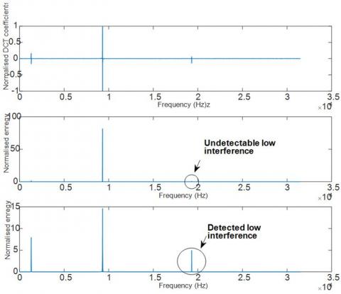
where, [R(k)] is the normalized kth DCT magnitude, w is the analysis window length. The use of the Shannon energy rather of squared energy is due to its ability to detect low interference peaks better than the classical squared energy. This feature allows detection and, therefore, reduction of both low and high interference peaks [24].
Figure 1 confirms the ability of Shannon energy based envelope detector compared to the conventional squared energy detector.
Figure 1. Detection performance comparison. The DCT of contaminated signal (Top), the conventional squared energy detector (middle), and the Shannon energy based envelope detector (bottom)
The proposed interference mitigation unit is embedded in the pre-dispreading part of the GNSS receiver (Figure 2). The suggested technique is constituted of three blocks. The first block is employed to obtain the frequency representation by DCT transform application on the signal r(n). Consequently, the detection and characterization of the interference RFI is the task of the second block. Finally, the excision of the interference signal existing in the GNSS signal is done by the use of a DFS-based notch filter in the third block. The frequency representation leads to an accurate interference detection and mitigation. However, the performance of the two first blocks have a significant impact on the performance of the third blocks.
For more illustration of the suggested approach, a flowchart is shown in Figure 3. Note that SE(k) and THSE(k) are respectively, Shannon energy-based envelope detector signal and its thresholded version.
Figure 2. Scheme of the proposed GNSS interference detection and mitigation unit
Figure 3. The flowchart of the CWI detection and mitigation unit
4.1 Signal transformation in the frequency domain by DCT application
The phase of the frequency transform of the incoming interfered GNSS signal is ensured by the first block of the mitigation unit. This phase is established by the DCT transform. Thus, the output of the block is a transformed vector of the GNSS contaminated signal.
4.2 Interferences detection and characterization
The crucial detection step decides whether an interference signal exists or not. It is constituted of two stages:
The first stage consists in the adequate threshold determination. Accordingly, the implemented method detects interfering signals by monitoring the receiver pre-correlation noise level. As it is well known, the received signal power level is below an expected thermal noise. As a result, we can use this important feature to estimate a suitable threshold level involving the Shannon-energy envelope detector (in relation with the noise level), in the DCT-domain. It is worth noting that after a sufficient set of measures (more than 100), one can determine, empirically, a predefined threshold magnitude (noise variance) discriminating the interference absence case from the opposite one.
The second stage consists in the use of a moving window Shannon energy (MWSE) operator to detect and localize the interference position. It means that the MWSE calculates the Shannon energy for each kth sample based on the magnitude of the sample itself and the surrounding neighbors. It is noticeable that an adequate choice of the processing moving window length brings out an accurate envelope, which leads to a precise localization of the interference frequencies.
To more refine the resulting envelope, we employed a Median filter as a smoother.
Note that each mth interference band (in the case of M tones) is concentrated around a central interference frequency $f_{i n terf_{m}}$ according to Eq. (11):
$f_{\text {int } e r_{\text {band _ } m}}=L b_{m} . ., f_{\text {int } e r f_{m}}, . . U b_{m}$
$1 \leq m \leq M$ (11)
where: $L b_{m}$ and $U b_{m}$ are respectively the upper and lower borders around the $f_{interf_{m}}$. When M=1, we are in the case of single tone interference.
4.3 Interference mitigation by DFS-based notch filter
In this stage, the interference excision is performed by the use of DFS-based notch filter. This method allows us to mitigate accurately the interference, due to the fact that the DFS orthogonal base is the ideal base for pure sinusoids representation (projection), which is the case of the CWI. Consequently, a frequency band rejection around each central interference frequency ${f_{{interf}}}_{m}$ is achieved according to Eq. (11), where the lower and the upper borders are expressed in (12):
$\left\{\begin{array}{l}L b_{m}=f_{ {interf }_{m}}-\alpha \times f_{0} \\ U b_{m}=f_{ {interf}_m}+\alpha \times f_{0}\end{array}\right.$ (12)
Note that the respective frequency indexes KLbm and KUbmof the mth interferences are shown in Eq. (13)
$\left\{\begin{array}{l}K_{L b m}=\left\lfloor\frac{f_{\text {int}{erf}_{m}}-\alpha \times f_{0}}{f_{0}}\right\rfloor=\left\lfloor\frac{f_{\text {int}{erf}_m}}{f_{0}}\right\rfloor-\alpha \\ K_{U b m}=\left\lfloor\frac{f_{\text {int}{erf}_m}+\alpha \times f_{0}}{f_{0}}\right\rfloor=\left\lfloor\frac{f_{\text {int}{erf}_m}}{f_{0}}\right\rfloor+\alpha\end{array}\right.$ (13)
where, α is a width index.
Accordingly, the coefficients ak and bk $\left(K_{L b m} \leq k \leq K_{U b m}\right)$ corresponding to all harmonics belonging to the mth CWIs, are calculated by the use of the equation previously mentioned in Eq. (9). Logically following, each interference is estimated by the summation of all the harmonics belonging to $f_{{inter}_{band}}$ interval. The estimated harmonics interference is removed from the input signal by simple subtraction. The proposed algorithm can be summarized in:
Step 1: for each mthinterference (1≤m≤M), determinate KLbmand KUbmaccording to (13).
Step 2: Calculation of the appropriate akand bk belonging the interval [KLbm,KUbm] according to (9).
Step 3: Estimation of the RFI by the summation of all harmonics corresponding to the founded interval.
Step 4: Mitigation of the estimated RFI by its subtraction from the contaminated signal.
Note that this procedure is done for all the contaminating RFI. Accordingly, this strategy is suitable for both single and multi-tone interferences cases.
In order to evaluate the performance of the suggested approach applied in the GNSS receiver, the mitigation algorithm has been implemented as user defined integrated block in a MATLAB-based simulator ‘GE5-TUT’, which is dedicated to the Galileo E5 band [25]. As previously mentioned, the new GNSS signals like GPS, European Galileo, and others are considered as DSSS communications systems [1, 6, 11]. For this reason, the interferences mitigation methods are suitable for all systems of satellite navigation. Accordingly, the proposed method will be applied on the European Galileo E5 signal. It is constituted of two bands, the first one is the E5a band centered at 1176.45 MHz and the second one named by E5b band centered at 1207.140 MHz, both are modulated by an AltBOC (15,10) procedure with a chipping rate of 10.23 Mbps [25].
The designed mitigation method considers that the received signal is corrupted by a SCWI (in a first situation) and by a MCWI (in the second situation) at several graduated power levels. Additionally, it is worthy to note that like the others GNSS systems, the Galileo E5a signal is immersed within AWGN due to their weakness.
Consequently, the signal parameters description is reported in Table 1. The used metrics to evaluate performance of the suggested algorithm and to situate it among some state-of-the-art works are given in Table 2.
Table 1. E5aI signal parameters
|
Parameter |
Value |
|
Desired signal |
Galileo E5a-I |
|
Sampling frequency fs |
31.500 MHz |
|
Intermediate frequency fIF |
4.655 MHz |
|
Coherent integration |
1ms |
|
CNR |
49 dB-Hz |
Table 2. Metrics used to evaluate the performance of the proposed method
|
Metrics |
|
PSDs of the signal before and after the interference reduction [5, 7, 18]. |
|
The ambiguity function S(τ,Fd) which results from The satellite acquisition operation [6, 13, 18]. |
|
The correlation coefficient showing how is the degree of similitude between the retrieved signal and the original clean signal [13]. It can be expressed as: $c=\frac{\sum_{i=1}^{N}(r-\bar{r})(\hat{r}-\overline{\hat{r}})}{\sqrt{\sum_{i=1}^{N}(r-\bar{r})^{2}} \sqrt{\sum_{i=1}^{N}(\hat{r}-\overline{\hat{r}})^{2}}}$ |
|
The acquisition ratio αmax meaning the ratio between the highest correlation peak P1 and the second highest correlation peak P2 of the accepted visible satellite [26, 27]. |
5.1 First situation: Single interference attenuation
The interference to signal ration ISR for both SCWI and MCWI cases is expressed by:
$I S R=10 \log \frac{I}{S}$
Note that the changing range of the ISR is 10-60 dB. Also S and I are the interference power and S is the useful signal power.
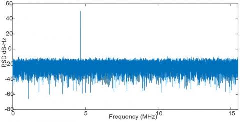
The used SCWI is positioned in the center of the main lobe at the intermediate frequency FI= 4.655 MHz of E5a band corresponding to carrier frequency of 1176.45 MHz. Accordingly, the Power Spectral Density (PSD) of the contaminated signal with 50 dB is shown in Figure 4.
In our approach, the detection and localization phase are performed in the first step of the process. The DCT transform and the Moving Window Shannon Energy (MWSE) (in the DCT domain) are achieved in order to detect and localize the frequency interference position in the assumed contaminated input signal.
Figure 4. PSD of the interfered input signal E5a for ISR=50dB
Figure 5. Detection phase results. The DCT transform application (top), interference frequency band to be rejected determination by the MWSE (middle) and the Median Filter Smoother output(bottom)
As a result, a range of frequencies (interval) around the central frequency of CW interference is founded. This latter, is well delimited (less widely) by the use of the Median Filter smoother (MFS). It means that the new smoothed band contains the central interference signal frequency (finterf), three frequencies components before finterfand three frequencies components after finterf. Figure 5 shows the obtained result from the application of the detection phase technique of the suggested method. The output of the median filter smoother gives
${{f}_{\operatorname{int}e{{r}_{band}}}}=\text{ }\left[ 4.652\text{ }4.653\text{ }4.654\text{ }4.655\text{ }4.656\text{ }4.6578\text{ }4.658 \right]\,\times {{10}^{6}}Hz$
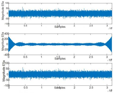
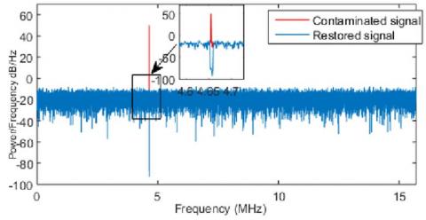
In order to ensure the removal of the center frequency interference finterf=4.6550 MHz decidedly, all of DCT coefficients related to the frequency band $f_{{{int er}_{band}}}$ will be nullified. However, the reduction of the CWIs by zeroing the DCT coefficients of the detected frequency band do not reduce borders effect, which causes serious problems, when performing the reconstruction phase by the inverse DCT transform. Therefore, the restoration of the uncontaminated signal is impossible due to the ripple’s accumulation. Thus, the inverse DCT transform is discarded in the reduction phase and the interference excision is achieved by the use of DFS-based notch filter. Figure 6 demonstrates visually the high efficiency of the DFS-based notch filter compared to the DCT-based notch filter.
Figure 6. The restoration of the uncontaminated signal. The uncontaminated signal (top), DCT-based notch fillter based (middle) and DFS- based notch filter (ISR=50 dB) (bottom)
Fo illustration, related to the first scenario, the calculation steps of $K_{L b}$ and $K_{U b}$ indexes are shown as following:
$T_{0}=N \times T_{s}$
where,
$N=31500, f_{s}=31500000 H z$
$f_{0}=1 / T_{0}[H z] \Rightarrow f_{0}=\left(\frac{f_{s}}{N}\right)=1000 H z$
$\left\{\begin{array}{l}L_{b}=4.6550 \times 10^{6}-(3 \times 1000) H z \\ U_{b}=4.6550 \times 10^{6}+(3 \times 1000) H z\end{array}\right.$
$\left\{\begin{array}{l}K_{L b}=4652 \\ K_{U b}=4658\end{array}\right.$
The next step is the calculation of corresponding Fourier series coefficients: ak and bk belonging to the band from KLb = 4652 to KUb = 4658. Figure 7 is a representation of the DFS spectral amplitude of the interference band harmonics to be suppressed.
From Figure 7, it is remarked from the panel that the central interference harmonic has an important value. Accordingly, from the bottom panel (zoom-in zone), it can be concluded that an efficient DFS-based notch filter can be realized by nullifying the DFS coefficients related to the central frequency in addition with the 3 adjacent harmonics before it and the 3 adjacent located after. The associated harmonics appropriate to the above-mentioned range (which produces an estimated version of the interference), are finally removed from the corrupted signal by a simple subtraction procedure.
Figure 7. The DFS spectral amplitude of interference harmonics band
Figure 8. The PSD before and after interference reduction (SCWI) (ISR=50dB)
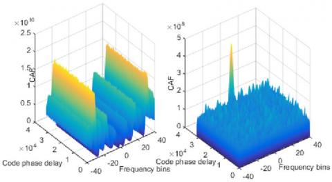
Figure 9. Ambiguity functions of the Galileo E5a signal affected by SCWI (ISR = 50dB). a) in presence of interference. b) after interference filtering
Figure 8 shows a comparison between the PSDs of received interfered signal before and after the interference mitigation unit.
For the aim of performance evaluation and efficiency comparison, the adaptive second order IIR notch filtering, which is considered as a popular technique and the most common interference countermeasure [10, 25-27], the Wavelet Packet Decomposition WDP based filtering algorithm for jamming reduction [6, 18, 28] and the DCT-based notch filter method are faced to the suggested DFS-based notch filter. Figure 9 shows the impact of the proposed mitigation method on the ambiguity function S(τ,Fd). The acquisition search spaces are obtained using 1ms of coherent integration and two non-coherent integrations. As it can be seen from the Figure 9(a), that in the case if the presence of the SCWI (50 dB), the ambiguity function obtained from the contaminated signal do not shows a correlation peak which leads to the wrong estimation of acquisition parameters. Therefore, the satellite is invisible by the receiver. Conversely, as shown the Figure 9(b) that presents a peak of the correlation function that validates the DFS-based notch filter effectiveness.
Knowing that αmax is a measure deduced from the acquisition search space, it indicates the signal strength of a visible satellite, the Table 3 gives some informative results.
Table 3 shows that the αmax of the retrieved signal by the DFS-based notch filter, has a slight greater value compared to the corresponding one of the signals retrieved by the conventional IIR notch filter and the WDP based filtering method.
For more consolidation of the effectiveness of the proposed approach, by results, we use the correlation coefficient as a metric. Consequently, the compared conventional methods to our suggested DFS-based notch filter strategy are respectively: DCT-based notch filter, IIR second order notch filter and WPD-based filter algorithm. Figure 10 illustrates the efficiency of our technique.
Table 3. Acquisition ratio after interference removal for SCWI
|
Interference mitigation method |
αmax |
|
IIR notch filter |
1.93 |
|
Proposed DFS-based notch filter |
2.20 |
|
WPD-based filter method |
1.97 |
5.2 Second situation: Multi interferences reduction
The second situation is the interference reduction of Multi CWIs. Accordingly, 3 interferences are added corrupting wider frequency band than the main lob. Like the previous situation, the first step consists in the detection and localization of the different positions of existing interferences in the input signal. The detected bands (by DCT, MWSE envelope detector and Median filter) that contains interferences and that must be rejected:
${{f}_{\operatorname{int}er}}_{_{band1}}=\left[ 1.652\,\,1.653\,\,1.654\,\,1.655\,\,1.656\,\,1.657\,\,1.658 \right]\times {{10}^{6}}Hz$
${{f}_{\operatorname{int}er}}_{_{band2}}=\left[ 4.652\,\,4.653\,\,4.654\,\,4.655\,\,4.656\,\,4.657\,\,4.658 \right]\times {{10}^{6}}Hz$
${{f}_{\operatorname{int}er}}_{_{band1}}=\left[ 9.652\,\,9.653\,\,9.654\,\,9.655\,\,9.656\,\,9.657\,\,9.658 \right]\times {{10}^{6}}Hz$
The corresponding borders for each contaminated band are respectively:
$\left\{\begin{array}{l}L b_{1}=1.655 \times 10^{6}-(3 \times 1000) H z \\ U b_{1}=1.655 \times 10^{6}-(3 \times 1000) H z\end{array}\right.$
$\left\{\begin{array}{l}L b_{2}=4.655 \times 10-(3 \times 1000) H z \\ U b_{2}=4.655 \times 10^{6}+(3 \times 1000) H z\end{array}\right.$
$\left\{\begin{array}{l}L b_{3}=9.655 \times 10^{6}-(3 \times 1000) H z \\ U b_{3}=9.655 \times 10^{6}+(3 \times 1000) H z\end{array}\right.$
The harmonics indexes $K_{L b_{m}}$ and $K_{L b_{m}}$ (m=1,2,3) of the interferences bands are expressed as:
$\left\{\begin{array}{l}K_{L b 1}=1652 \\ K_{U b 1}=1658\end{array}\right.$
$\left\{\begin{array}{l}K_{L b 2}=4652 \\ K_{U b 2}=4658\end{array}\left\{\begin{array}{l}K_{L b 3}=9652 \\ K_{U b 3}=9658\end{array}\right.\right.$
Figure 10. Comparative results using the correlation coefficient (SCWI case)
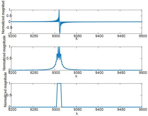
Similarly as in the first scenario, the next step is the calculation of Fourier series coefficients: ak, bk belonging to [1652 to 1658], [4652 to 4658] and [9652 to 9658]. Figure 11 shows that the coefficients of the central frequencies of the interferences have an important value. Therefore, The DFS-based notch filter can be realized by nullifying the DFS coefficients related to the central frequencies in addition with the 3 adjacent harmonics before it and the 3 adjacent situated after (the zoomed zone). Next, a summation of all harmonics corresponding to the aforementioned intervals is achieved. Accordingly, the estimated version of the interferences are finally removed from the corrupted signal by a simple subtraction. Figure 11 shows a comparison between the PSDs of received interfered signal and the signal after the interference mitigation unit.
As previously mentioned in the first situation, the ambiguity functions of the corrupted signal and the retrieved signal after the interference mitigation unit are given in the Figure 12. From the acquisition search space, αmax is indicated in Table 4 and provides some confirming results.
Also, the correlation coefficient metric, demonstrates the efficiency of our method in the case of MCWI scenario as shown in the Figure 13.
Table 4. Acquisition ratio after interference removal for MCWI
|
Interference mitigation method |
αmax |
|
IIR notch filter |
1.73 |
|
Proposed DFS-based notch filter |
2.02 |
|
WPD based filter method |
1.781 |
Figure 11. The PSD before and after interference mitigation (MCWI) (ISR=50dB) (top), Zoom - In (bottom)
Figure 12. Ambiguity functions of the Galileo E5a affected by MCWI (ISR = 50 dB). a) in presence of interference. b) after interference filtering
Figure 13. Comparative results based on the correlation coefficient (MCWI)
It can be reported that the suggested method shows a stable ability of interference reduction in case of both weak and strong interferences contamination. Adorningly, the proposed strategy presents superior performance compared to the faced methods in the case of strong interferences contamination.
In this paper, a new and efficient approach involving the combination of, the Shannon energy-based envelope detection in the DCT domain and DFS-based notch filter, for CWI detection and mitigation in the GNSS receivers, is proposed. Therefore, an accurate detection and localization of the interference is guaranteed by the use of the DCT followed by the Shannon energy-based envelope detector allowing the detection of both the strong and weak interferences. However, a high precision interference excision is achieved by the DFS-based notch filter. Finally, the efficiency of the conceived approach is validated by presenting a comparative study facing the proposed algorithm to the IIR second order notch filter, the WDP based filtering algorithm and the DCT-based notch filter.
[1] Kaplan, E., Hegarty, C. (2017). Understanding GPS/GNSS: Principles and Applications. Artech House.
[2] Marzec, P., Kos, A. (2021). Thermal navigation for blind people. Bulletin of the Polish Academy of Sciences: Technical Sciences, 69(1): e136038-e136038. http://doi.org/10.24425/bpasts.2021.136038
[3] Bastide, F., Chatre, E., Macabiau, C. (2001). GPS interference detection and identification using multicorrelator receivers. In Proceedings of the 14th International Technical Meeting of the Satellite Division of The Institute of Navigation (ION GPS 2001), Salt Lake City, UT, pp. 872-881.
[4] Mosavi, M.R., Shafiee, F. (2016). Narrowband interference suppression for GPS navigation using neural networks. GPS Solutions, 22(3): 341-351. https://doi.org/10.1007/s10291-015-0442-8
[5] Chien, Y., Huang, Y., Yang, D., Tsao, H. (2010). A novel continuous wave interference detectable adaptive notch filter for GPS receivers. 2010 IEEE Global Telecommunications Conference GLOBECOM, Miami, FL, USA, pp. 1-6. https://doi.org/10.1109/GLOCOM.2010.5684115
[6] Mosavi, M.R., Rezaei, M.J., Pashaian, M., et al. (2017). A fast and accurate anti-jamming system based on wavelet packet transform for GPS receivers. GPS Solution, 21: 415-426. https://doi.org/10.1007/s10291-016-0535-z
[7] Konovaltsev, A., Lorenzo, D. S. D., Hornbostel, A., Enge, P. (2008). Mitigation of continuous and pulsed radio interference with GNSS antenna arrays. Proceedings of the 21st International Technical Meeting of the Satellite Division of The Institute of Navigation (ION GNSS 2008), Savannah, GA, pp. 2786-2795.
[8] Higgins, T., Webster, T., Shackelford, A.K. (2014). Mitigating interference via spatial and spectral nulling. IET Radar Sonar Navigation, 8(2): 84-93, https://doi.org/10.1049/iet-rsn.2013.0194
[9] Bastide, F., Akos, D., Macabiau, C., Roturier, B. (2003). Automatic gain control (AGC) as an interference assessment tool. Proceedings of the 16th International Technical Meeting of the Satellite Division of The Institute of Navigation (ION GPS/GNSS’03), Portland, OR, pp. 2042-2053.
[10] Borio, D., Camoriano, L., Presti, L.L. (2008). Two-pole and multi-pole notch filters: A computationally effective solution for GNSS interference detection and mitigation. IEEE System Journal, 2(1): 38-47 https://doi.org/10.1109/JSYST.2007.914780
[11] Abdizadeh, M. (2013). GNSS signal acquisition in the presence of narrowband interference. Ph.D. thesis, Department of Geomatics Engineering, University of Calgary, Calgary, Canada.
[12] Capozza, P.T., Holland. B.J., Hopkinson, T.M., Landrau, R.L. (2000). A single-chip narrow-band frequency-domain excisor for the global positioning system (GPS) receiver. IEEE Journal of Solid-State Circuits, 35(3): 401-411. http://doi.org/10.1109/4.826823
[13] Khezzar, Z.A., Benzid, R., Saidi, L. (2020). New thresholding technique in DCT domain for interference mitigation in GNSS receivers. Traitement du Signal, 37(2): 169-180. https://doi.org/10.18280/ts.370203
[14] Borio, D., Camoriano, L., Savasta, S., Presti, L.L., (2008). Time-frequency excision for GNSS applications. IEEE Syst Journal, 2(1): 27-37. http://doi.org/10.1109/JSYST.2007.914914
[15] Zhang, Y.D., Amin, M.G. (2012). Anti-jamming GPS receiver with reduced phase distortions. IEEE Signal Processing Letters, 19(10): 635-638. http://doi.org/10.1109/LSP.2012.2209873
[16] Savasta, S., Lo Presti, L., Rao, M. (2013). Interference mitigation in GNSS receivers by a time-frequency approach. IEEE Transactions on Aerospace and Electronic Systems, 49(1): 415-438. http://doi.org/10.1109/TAES.2013.6404112
[17] Ouyang, X., Amin, M.G. (2001). Short-time Fourier transform receiver for nonstationary interference excision in direct sequence spread spectrum communications. IEEE Transactions on Signal Processing, 49(4): 851-863. http://doi.org/10.1109/78.912929
[18] Musumeci, L., Curran, J.T., Dovis, F. (2016). A Comparative analysis of adaptive a notch filtering and wavelet mitigation against jammers interference. Journal of the Institute of Navigation, 63(4): 533-550. https://doi.org/10.1002/navi.167
[19] Liu, Y., Ran, Y., Ke, T., Hu, X. (2012). Characterization of code tracking error of coherent DLL under CW interference. Wireless Personal Communications, 66(2): 397-417. https://doi.org/10.1007/s11277-011-0348-x
[20] Shin, H.S., Lee, C., Lee, M. (2010). Ideal filtering approach on DCT domain for biomedical signals: Index blocked DCT filtering method (IB-DCTFM). Journal of Medical Systems, 34(4): 741-753. https://doi.org/10.1007/s10916-009-9289-2
[21] Proakis, J.G., Manolakis, D.G. (2007). Digital signal processing: Principles, algorithms and applications, 4 edn. Prentice Hall Inc. Upper Saddle River.
[22] Sadhukhan, D., Pal, S., Mitra, M. (2015). Electrocardiogram data compression using adaptive bit encoding of the discrete Fourier transforms coefficients. IET Science, Measurement & Technology, 9(7): 866-874. http://doi.org/10.1049/iet-smt.2015.0013
[23] Bahaz, M., Benzid, R. (2018). Efficient algorithm for baseline wander and powerline noise removal from ECG signals based on discrete Fourier series. Australasian Physical and Engineering Sciences in Medicine, 41(1): 143-160. http://doi.org/10.1007/s13246-018-0623-1
[24] Beyramienanlou, H., Lotfivand, N. (2017). Shannon’s energy based algorithm in ECG signal processing. Computational and Mathematical Methods in Medicine, 2017: 8081361. http://doi.org/10.1155/2017/8081361
[25] de Diego, D.A., Ferrara, N., Nurmi, J., Lohan, E.S. (2016). Interference mitigation in the E5a Galileo band using an open-source simulator. Inside GNSS, 11(4): 55-63.
[26] Pashaian, M., Mosavi, M.R., Moghaddasi, M.S., Rezaei, M.J. (2016). A novel interference rejection method for GPS receivers. Iranian Journal of Electrical and Electronic Engineering, 12(1): 9-20. http://doi.org/10.22068/IJEEE.12.1.9
[27] Rusu-Casandra, A., Lohan, E.S., Seco-Granados, G., Marghescu, I. (2012). Investigation of narrowband interference filtering algorithms for Galileo CBOC signals. In Proceedings of the 3rd European Conference of Circuits Technology and Devices, ECCTD'12, Paris, France, pp. 274-279.
[28] Musumeci, L., Dovis, F. (2014). Use of the wavelet transform for interference detection and mitigation in global navigation satellite systems. International Journal of Navigation & Observation, 2014: 262186. http://doi.org/10.1155/2014/262186