Jie Yang
© 2022 IIETA. This article is published by IIETA and is licensed under the CC BY 4.0 license (http://creativecommons.org/licenses/by/4.0/).
OPEN ACCESS
In real scenes of sports competitions, interferences like light intensity and camera jitter make it difficult to accurately segment and identify the action information in the complex continuous actions of athletes. Spiking, a common action in volleyball, can be divided into three closely correlated phases: landing, buffering, and stretching. This paper explores the image segmentation of the continuous action of spiking in volleyball based on spatial neighborhood information. Specifically, the authors detailed how to acquire the neighborhood correlation images of volleyball players spiking the ball. The framework of the image segmentation model was presented, and the extraction method of weighted spatial neighborhood information was expounded. Next, the fuzzy c-means (FCM) clustering was optimized to effectively segment the video images on the continuous action of spiking in volleyball. The proposed algorithm was proved valid through experiments.
spatial neighborhood information, the continuous action of spiking in volleyball, image segmentation, fuzzy c-means (FCM) clustering
Volleyball is one of the most popular ball sports. Spiking, a common action in volleyball, refers to the transition from run-up to jumping in the predetermined direction. It can be divided into three closely correlated phases: landing, buffering, and stretching [1-4]. During landing, the landing resistance should be minimized to create conditions for jumping. The buffering determines the jumping effect. During buffering, the player needs to bend the upper knee as much as possible to increase the contraction strength and speed of each joint of the body. During stretching, the legs and the arms should swing coordinately. The more explosive the action, the greater the jumping height [5-9].
Sports videos can intuitively record a series of scenes of athletes’ continuous actions during sports, and contain an abundance of high-level semantic information [10-14]. In real scenes of sports competitions, interferences like light intensity and camera jitter make it difficult to accurately segment and identify the action information in the complex continuous actions of athletes [15-19].
The existing sports video image segmentation methods have defects like coarse segmentation, and high spatial distortion rate. Li and Chang [20, 21] proposed a sports video image segmentation method based on fuzzy clustering algorithm. Using the time-domain difference image, second-order fuzzy attribute was established with normal distribution and gravity value, along with the membership function of the fuzzy attribute. Then, fuzzy clustering was performed on the time-domain difference image, and edge detection was carried out to segment sports video images. There is a high demand for editing, segmenting, and integrating sports videos. Calandre et al. [22] introduced the results of the 2020 sports video annotation task of “stroke detection in table tennis”. The annotation plan is based on actions, the most pronounced performance of players. The action information was captured at the image level by optical flow, and aggregated at the sequence level by dynamic images encoding temporal information. On this basis, a multi-flow structure was provided, and the table tennis strokes were detected in combination with red-green-blue (RGB)-based dynamic images, optical flow-based dynamic images, and RGB frames. Du [23] explored the three-dimensional (3D) dynamic simulation of sports video image series through image frame acquisition, algorithm design, to computer simulation and analysis. The purpose is to verify the superiority and feasibility of their factoring algorithm in 3D dynamic simulation. According to the features of football videos and video assistant referee (VAR), Han [24] presented an algorithm that quickly segments and tracks the players in videos. According to the complementary advantages of RGB space and hue-saturation-intensity (HSI) space, the main and auxiliary spaces were combined to segment objects in video. The results were compared with the normalized color histogram of each object to determine the team of each player.
There are many successful video action recognition algorithms. But their effectiveness is largely validated on public datasets. In addition, the images on athletes’ sports actions are often from a single segment of the video, which is a far cry from the actual scenes of spiking in volleyball. Therefore, it is very necessary to recognize the continuous actions of the human body based on deep neural networks (DNNs), and apply the networks to the actual environment of spiking of volleyball players. Taking the continuous action of spiking in volleyball for example, this paper studies an image segmentation algorithm based on spatial neighborhood information. Section 2 details the acquisition method of neighborhood correlation images of volleyball players spiking the ball. Section 3 illustrates the framework of the image segmentation model, and expounds on the extraction method of weighted spatial neighborhood information. Section 4 optimizes the fuzzy c-means (FCM) clustering to effectively segment the video images on the continuous action of spiking in volleyball. The proposed algorithm was proved valid through experiments.
To obtain the neighborhood correlation images on the spiking action of volleyball players, a 3×3 dynamic window was opened at the position of spiking in two time-phase images. The correlation coefficient, slope, and intercept are denoted by χ, κ, and ζ, respectively. The covariance of the brightness in all bands of the window is denoted by BBC. The standard deviations of the brightness of all bands in the windows corresponding to the previous and current time phases are denoted by r1 and r2, respectively. The brightness of the l-th pixel in the windows corresponding to the previous and current time phases are denoted by YUl,1 and YUl,2, respectively; the total number of pixels in all bands of the window is denoted by m; the mean brightness of all bands in the windows corresponding to the previous and current time phases are denoted by v1 and v2, respectively. Then, the χ, κ, and ζ of the neighborhood corresponding to each window can be computed by:
$BBC=\frac{\sum\limits_{l=1}^{m}{\left( Y{{U}_{l,1}}-{{v}_{1}} \right)\left( Y{{U}_{l,2}}-{{v}_{2}} \right)}}{m-1}$ (1)
$\chi =\frac{cov}{{{r}_{1}}{{r}_{2}}}$ (2)
$\kappa =\frac{cov}{r_{1}^{2}}$ (3)
$\zeta =\frac{\sum\limits_{l=1}^{m}{Y{{U}_{l,2}}}-\kappa \sum\limits_{l=1}^{m}{Y{{U}_{l,1}}}}{m}$ (4)
The three values are assigned to the center position of the dynamic window. Then, it is possible to create the neighborhood correlation image around the center of the dynamic window.
This paper treats χ and κ as their difference from 1, and visualizes ζ as its difference from 0. In this way, the dynamic parts and constant parts of the continuous action image on volleyball spiking can be represented by bright pixels and dark pixels, respectively.
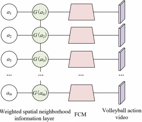
Figure 1 shows the framework of the image segmentation model. It can be seen that, prior to image segmentation, the weighted spatial neighborhood information is extracted. For the target continuous action image on volleyball spiking, any pixel aj is affected differently by different pixels in its neighborhood MY(aj). Let FC(aj,ai) be a weight reflecting the degree of influence of neighborhood pixel ai over aj. Then, the weighted neighborhood information can be calculated by:
Figure 1. Image segmentation model
$g\left( {{a}_{j}} \right)=\sum\limits_{i\in MY\left( {{a}_{j}} \right)}{FC\left( {{a}_{j}},{{a}_{i}} \right)}{{a}_{i}}$ (5)
The idea of fuzzy clustering is introduced to obtain more proper weighted neighborhood information. The fuzzy membership, which is equivalent to weight, can be calculated by:
$FC\left( {{a}_{j}},{{a}_{i}} \right)=v\left( {{a}_{j}},{{a}_{i}} \right)={{\left( {{\sum\limits_{i\in MY\left( {{a}_{j}} \right)}{\left( \frac{{{\left\| {{a}_{j}}-{{a}_{i}} \right\|}^{2}}}{{{\left\| {{a}_{j}}-{{a}_{i}} \right\|}^{2}}} \right)}}^{1/\left( n-1 \right)}} \right)}^{-1}}$ (6)
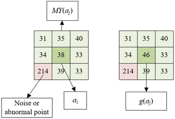
Taking the center pixel aj as the cluster center, then weight FC(aj,ai) is the membership v(aj,ai) of ai relative to aj. The value of FC(aj,ai) is negatively correlated with the distance between ai and aj, and positively correlated with v(aj,ai). Figure 2 illustrates the weighted mean of the neighborhood.
Figure 2. Weighted mean of the neighborhood
This paper optimizes the FCM to effectively segment the images on the continuous action of volleyball spiking. The optimized FCM employs the mean shift algorithm to pinpoint the densest sample information in the image feature space. Based on the neighborhood correlation image acquired in the preceding section, the weight of each neighborhood image block is solved. Then, the detailed information of continuous images is obtained by weighted fuzzy factor. Figure 3 shows the framework of the image segmentation model.
Figure 3. Framework of image segmentation model
Suppose the image on the continuous action of volleyball spiking A={a1,a2,...,am} contains m pixels. Let f be the bandwidth of the gray value domain of the image; l'(a) be the gradient of the kernel function, which satisfies h(a)=-l'(a). Then, the mean shift vector of the mean shift algorithm can be calculated by:
${{N}_{H}}\left( a \right)=\frac{\sum\limits_{i=1}^{m}{{{a}_{i}}h\left( {{\left\| \left( a-{{a}_{i}} \right)/f \right\|}^{2}} \right)}}{\sum\limits_{i=1}^{m}{h\left( {{\left\| \left( a-{{a}_{i}} \right)/f \right\|}^{2}} \right)}}-a$ (7)
The new shift center nH(a) can be calculated by:
${{n}_{H}}\left( a \right)=\frac{\sum\limits_{i=1}^{m}{{{a}_{i}}h\left( {{\left\| \left( a-{{a}_{i}} \right)/f \right\|}^{2}} \right)}}{\sum\limits_{i=1}^{m}{h\left( {{\left\| \left( a-{{a}_{i}} \right)/f \right\|}^{2}} \right)}}$ (8)
For the image on the continuous action of volleyball spiking, the neighborhood image blocks corresponding to the neighborhood correlation images contain much information about the neighborhood, and mirror the features of the continuous action of spiking. For the image on the continuous action of volleyball spiking A={a1,a2,...,am}, every pixel ai has ti={Tiw,w∈Mi} neighborhood image blocks, where Mi is the s-order neighborhood of ai. Due to the presence of many noises and abnormal points in video images, the pixels in the neighborhood image blocks formed by different neighborhood correlation images were assigned different weights.
Let aw be the center pixel in the image ti on the continuous action of volleyball spiking; aw' be the other pixels in each neighborhood image block; mi be the number of pixels in a neighborhood image block; ti be the neighborhood image block corresponding to ai. Then, the variance of pixels in ti can be calculated by:
${{\xi }_{iw}}={{\left[ \frac{\sum\limits_{w'\in {{M}_{i}}\backslash \left\{ w \right\}}{{{\left( {{a}_{w'}}-{{a}_{w}} \right)}^{2}}}}{{{m}_{i}}-1} \right]}^{\frac{1}{2}}}$ (9)
By Gaussian kernel function, the variance is mapped to the kernel space:
${{\delta }_{iw}}=exp\left[ -\left( {{\xi }_{iw}}-\frac{\sum\limits_{w\in {{M}_{i}}}{{{ \quad \xi }_{iw}}}}{{{m}_{i}}} \right) \right]$ (10)
The weights of all pixels in the neighborhood image block are normalized by:
${{\eta }_{iw}}=\frac{{{\delta }_{iw}}}{\sum\limits_{w\in {{M}_{i}}}{{{\delta }_{iw}}}}$ (11)
The traditional image segmentation algorithm has a low segmentation accuracy, because video images contain some nonnegligible noises and abnormal points. To solve the problem, this paper relies on the weighted fuzzy factor to characterize the information in the image on the continuous action of volleyball spiking. Let vlj be the fuzzy membership matrix; ul be the cluster center; ηij be the weight. For any image pixel ai, the weighted fuzzy factor can be calculated by:
${{H}_{li}}=\sum\limits_{j\in MY\left( {{a}_{i}} \right),j\ne i}{{{\eta }_{ij}}{{\left( 1-{{v}_{lj}} \right)}^{n}}}{{\left\| {{a}_{i}}-{{u}_{l}} \right\|}^{2}}$ (12)
The value of ηij covers two parts: spatial distance weight and spatial intensity weight. By fully utilizing the two weights, the spatial information in the image on the continuous action of volleyball spiking could be realized, which contributes to the robustness of the image segmentation algorithm.
The spatial distance weight of ηij represents the location constraint of any image pixel ai. Let cijr be the Euclidean distance between pixel ai and neighborhood pixel aj. Then, the spatial distance weight can be calculated by:
${{\eta }_{rc}}=\frac{1}{{{c}^{r}}+1}$ (13)
Almost all the information of the center pixel can be represented by the s-order neighborhood of the pixels in the image on the continuous action of volleyball spiking. Therefore, this paper determines the spatial distance weight based on the local information of the image.
The spatial intensity weight of ηij is defined as the gray value ratio of pixels in the neighborhood of any image pixel ai. Let ai and aj denote a pixel in the image on the continuous action of volleyball spiking, and a neighborhood pixel of that pixel, respectively. Then, the s-order neighborhoods MYi and MYj of ai and aj can be selected to define the spatial intensity distance of pixel ai as:
$c_{ij}^{I}=\frac{1}{{{s}^{2}}}\sum\limits_{l=1}^{{{s}^{2}}}{\frac{{{I}_{M{{Y}_{i}}}}\left( l \right)}{{{I}_{M{{Y}_{j}}}}\left( l \right)}}$ (14)
The spatial intensity weight is mapped to the natural logarithm space:
${{\eta }_{ic}}=1-log\left( c_{ij}^{I} \right)$ (15)
The weight of the weighted fuzzy factor can be defined as:
${{\eta }_{ij}}={{\eta }_{rc}}\cdot {{\eta }_{ic}}$ (16)
Let vli be the membership matrix; n be the fuzzy parameter; ηis be the weight of the neighborhood image block corresponding to pixel ai; SUis be a pixel in the neighborhood image block corresponding to pixel ai; ul be the cluster center; Hli be the weighted fuzzy factor. Based on Hli, the objective function of our image segmentation algorithm can be defined as follows:
${{J}_{MSIFCM}}=\sum\limits_{i=1}^{m}{\sum\limits_{l=1}^{d}{v_{li}^{n}\sum\limits_{s\in {{M}_{i}}}{{{\eta }_{is}}{{\left\| S{{U}_{is}}-{{u}_{l}} \right\|}^{2}}}+{{H}_{li}}}}$ (17)
The objective function is minimized by the Lagrange multiplier method. Let MYi be the set of neighborhood pixels of pixel ai; v'li be the smoothed membership function; ψij∈ [0,1] be the neighborhood pixel weight coefficient controlling the influence of neighborhood pixels on the center pixel; vli be the updated membership. Then, the membership can be updated by:
${{v}_{li}}={{\left\{ \sum\limits_{k=1}^{d}{\left[ {{\left( \frac{\sum\limits_{s\in {{M}_{i}}}{{{\eta }_{is}}{{\left( S{{U}_{is}}-{{u}_{l}} \right)}^{2}}+{{H}_{li}}}}{\sum\limits_{s\in {{M}_{i}}}{{{\eta }_{is}}{{\left( S{{U}_{is}}-{{u}_{j}} \right)}^{2}}+{{H}_{ji}}}} \right)}^{\frac{1}{n-1}}} \right]} \right\}}^{-1}}$ (18)
The cluster center can be updated by:
${{u}_{l}}=\frac{\sum\limits_{i=1}^{m}{v_{li}^{n}\sum\limits_{s\in {{M}_{i}}}{{{\eta }_{is}}S{{U}_{is}}}}}{\sum\limits_{i=1}^{m}{v_{li}^{n}\sum\limits_{s\in {{M}_{i}}}{{{\eta }_{is}}}}}$ (19)
The membership can be smoothened by:
$v_{li}^{'}=\sum\limits_{j\in {{M}_{i}}}{{{\psi }_{ij}}{{v}_{li}}}$ (20)
Let aav and ξi be the mean and variance of the neighborhood pixels of pixel ai, respectively; UC(ai,aj) be the control coefficient. Then, the weight coefficient of each neighborhood pixel can be calculated by:
${{\psi }_{ij}}=\left\{ \begin{align} & UC\left( {{a}_{i}},{{a}_{j}} \right),\left| {{a}_{i}}-{{a}_{av}} \right|<{{\xi }_{i}} \\ & 0,\left| {{a}_{i}}-{{a}_{av}} \right|>{{\xi }_{i}} \\\end{align} \right.$ (21)
The segmentation effect is measured by Euclidean distance. The control coefficient UC(ai,aj) can be calculated by:
$UC\left( {{a}_{i}},{{a}_{j}} \right)=\frac{c\left( {{a}_{i}},{{a}_{j}} \right)}{\sum\limits_{k\in {{M}_{i}}}{c\left( {{a}_{i}},{{a}_{j}} \right)}}$ (22)
The distance from the center pixel ai to a neighborhood pixel aj is negatively correlated with the influence of aj over ai. Hence, the control coefficient UC(ai,aj) is defined as the Euclidean distance ratio between the two pixels. The closer the UC(ai,aj) is to one, the stronger the correlation between aj and ai. The further the UC(ai,aj) is from one, the weaker the correlation. Based on Euclidean distance, the above differentiation of pixel correlation effectively clarifies the degree of impacts of each pixel in the image on the continuous action of volleyball spiking over the weight coefficient, making the clustering of the continuous action of volleyball spiking more accurate.
Table 1 compares the accuracies of different image segmentation algorithms on volleyball action video images, which were added with different levels of noises. The reference algorithms include threshold-based algorithm, edge-based algorithm, wavelet transform-based algorithm, mathematical morphology-based algorithm, and genetic algorithm-based algorithm.
The additive Gaussian white noises all had a mean of zero. The pulse noises were of the intensities of 0.1, and 0.2, respectively. The mixed noise was mixed from Gaussian white noise 2 and pulse noise 1. As shown in Table 1, with the growing intensity of noises, our algorithm always outperformed the other algorithms in image segmentation accuracy. Hence, our algorithm can ideally and robustly segment noisy images on volleyball actions.
Table 2 shows the distribution coefficients and distribution entropies of volleyball video images with Gaussian white noise 1 and pulse noise 1. As can be seen from the table, the distribution coefficients were smaller than 0.9 on the image added with the Gaussian white noise. But the distribution coefficient of our algorithm was the closest to 1, and the distribution entropy of our algorithm was the nearest to 0. On the image added with the Gaussian white noise, the distribution coefficient (0.9547) of our algorithm was higher than that of any other algorithm. The distribution entropies of the algorithm based on mathematical morphology, the algorithm based on genetic algorithm, and our algorithm were smaller than 0.1. Hence, our algorithm is not very sensitive to the noises in volleyball action video images, and could ideally segment such images.
Table 1. Accuracies of different image segmentation algorithms
|
Noise |
Gaussian white noise 1 |
Gaussian white noise 2 |
Pulse noise 1 |
Pulse noise 2 |
Mixed noise |
|
Threshold-based algorithm |
65.12 |
59.62 |
98.36 |
93.17 |
65.19 |
|
Edge-based algorithm |
95.27 |
83.05 |
92.58 |
90.36 |
84.53 |
|
Wavelet transform-based algorithm |
92.64 |
85.48 |
94.51 |
92.04 |
94.79 |
|
Mathematical morphology-based algorithm |
74.69 |
53.12 |
95.02 |
98.57 |
86.03 |
|
Genetic algorithm-based algorithm |
96.18 |
93.47 |
92.18 |
97.24 |
90.68 |
|
Our algorithm |
94.25 |
96.35 |
93.52 |
96.27 |
96.53 |
Table 2. Distribution coefficients and distribution entropies of different noises
|
Noise |
Gaussian white noise 1 |
Pulse noise 1 |
||
|
Index |
Distribution coefficient |
Distribution entropy |
Distribution coefficient |
Distribution entropy |
|
Threshold-based algorithm |
0.7526 |
0.5218 |
0.9362 |
0.1529 |
|
Edge-based algorithm |
0.7482 |
0.4362 |
0.9485 |
0.1645 |
|
Wavelet transform-based algorithm |
0.7184 |
0.4629 |
0.9513 |
0.1327 |
|
Mathematical morphology-based algorithm |
0.7481 |
0.4261 |
0.9215 |
0.0481 |
|
Genetic algorithm-based algorithm |
0.8415 |
0.2635 |
0.9142 |
0.0958 |
|
Our algorithm |
0.9328 |
0.1362 |
0.9547 |
0.0615 |
Table 3. Segmentation errors of different algorithms on the images of the continuous action of volleyball spiking
|
|
Landing |
Buffering |
Stretching |
|
Threshold-based algorithm |
0.52% |
0.55% |
0.67% |
|
Edge-based algorithm |
0.55% |
0.52% |
0.81% |
|
Wavelet transform-based algorithm |
0.52% |
0.43% |
0.76% |
|
Mathematical morphology-based algorithm |
0.44% |
0.42% |
0.55% |
|
Genetic algorithm-based algorithm |
0.32% |
0.33% |
0.46% |
|
Our algorithm |
0.14% |
0.22% |
0.15% |
Figure 4. Example of volleyball action video images
Table 3 shows the segmentation errors of different algorithms on the images of the continuous action of volleyball spiking. It can be observed that our algorithm achieved the smallest errors (0.14%, 0.22%, and 0.15%) on segmenting the landing, buffering, and stretching phases of the continuous spiking action. This proves that our algorithm can effectively eliminate the noise effect in segmenting noisy volleyball action video images, and improve the segmentation accuracy of the continuous action of volleyball spiking.
Figure 4 provides an example of volleyball action video images. The video contains a large variation in the view angle, and involves four single actions of volleyball spiking, namely, run-up, landing, buffering, and stretching.
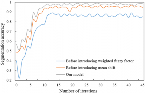
Figure 5. Segmentation accuracies before and after model optimization
This paper introduces the mean shift algorithm to pinpoint the densest sample information in the image feature space, computes the weight of each neighborhood image block based on the neighborhood correlation image, and derives the specific information of continuous images using the fuzzy factor. Figure 5 compares the segmentation accuracies before and after model optimization. After introducing the mean shift algorithm, the segmentation accuracy on the volleyball action video image set was higher than that of the original model. The introduction of the weighted fuzzy factor improved the accuracy by an even greater margin. The results show that our model extracted the greatest number of action features, realized the best performance, and thus the highest segmentation accuracy of the continuous action of volleyball spiking.
Figure 6. Recognition accuracies of each phase in the continuous action of volleyball spiking
Finally, this paper compares the recognition accuracies of our model on each phase of the continuous action of volleyball spiking (Figure 6). Although our model mainly targets the continuous action of volleyball spiking, it can detect each phase in that continuous action. As shown in Figure 6, the mean recognition accuracy of our model was greater than 80% on each phase. This further confirms the effectiveness of our model in recognizing each single sub-action of volleyball spiking.
This paper explores the image segmentation for the continuous action of spiking in volleyball based on spatial neighborhood information. After clarifying the framework of the image segmentation model, the authors detailed how to acquire the neighborhood correlation images of volleyball players spiking the ball. Next, the framework of the image segmentation model was presented, before expounding on the extraction method of weighted spatial neighborhood information. After that, the FCM was optimized to effectively segment the continuous action of spiking in volleyball. Through experiments, the authors compared the accuracies of different image segmentation algorithms on volleyball action video images added with different levels of noises. The results show that our algorithm can ideally and robustly segment noisy images on volleyball actions. After that, the authors summarized the distribution coefficients and distribution entropies of volleyball video images with Gaussian white noise 1 and pulse noise 1. It was learned that our algorithm is not very sensitive to the noises in volleyball action video images, and could ideally segment such images. In addition, the authors compared the segmentation errors of different algorithms on the images of the continuous action of volleyball spiking. The comparison shows that our algorithm can effectively eliminate the noises in noisy volleyball action video images. Finally, the segmentation accuracies before and after model optimization were presented, which demonstrate that our model extracted the greatest number of action features, realized the best performance, and thus the highest segmentation accuracy of the continuous action of volleyball spiking.
[1] Garcia, S., Rao, G., Berton, E., Delattre, N. (2021). Foot landing patterns in experienced and novice volleyball players during spike jumps. Footwear Science, 13(S1): S76-S78. https://doi.org/10.1080/19424280.2021.1917690
[2] Gupta, D., Jensen, J.L., Abraham, L.D. (2021). Biomechanics of hang-time in volleyball spike jumps. Journal of Biomechanics, 121: 110380. https://doi.org/10.1016/j.jbiomech.2021.110380
[3] Cheng, X., Li, Z., Du, S., Ikenaga, T. (2020). Body part connection, categorization and occlusion based tracking with correction by temporal positions for volleyball spike height analysis. IEICE Transactions on Fundamentals of Electronics, Communications and Computer Sciences, 103(12): 1503-1511. https://doi.org/10.1587/transfun.2020SMP0010
[4] Naito, K., Wakayama, A., Kubota, H., Maruyama, T. (2018). Energy distribution mechanism and open-kinetic-chain characteristics of the upper body system in female volleyball spiking. Proceedings of the Institution of Mechanical Engineers, Part P: Journal of Sports Engineering and Technology, 232(2): 79-93. https://doi.org/10.1177%2F1754337117700551
[5] Ding, J.L. (2014). Volleyball spiking point position and success rate correlation research based on biomechanical geometric model. BioTechnology: An Indian Journal, 10(4): 899-904.
[6] Zhou, Z.G. (2014). Volleyball spiking technique influence factors biomechanical model research and application. BioTechnology: An Indian, 10(7): 2010-2016.
[7] Wang, M., Liang, Z. (2021). An extraction method of volleyball spiking trajectory and teaching based on wireless sensor network. Security and Communication Networks, 2021: 9966994. https://doi.org/10.1155/2021/9966994
[8] Wang, Q. (2014). Volleyball best spike area research based on Lagrange extreme value analysis. BioTechnology: An Indian Journal, 10(2): 176-182.
[9] Mitchinson, L., Campbell, A., Oldmeadow, D., Gibson, W., Hopper, D. (2013). Comparison of upper arm kinematics during a volleyball spike between players with and without a history of shoulder injury. Journal of Applied Biomechanics, 29(2): 155-164.
[10] Tang, D. Z. (2013). A study of key technical factors of volleyball spike based on the biomechanical analysis. Information Technology Journal, 12(19): 5166-5171. https://dx.doi.org/10.3923/itj.2013.5166.5171
[11] Jiang, X., Wu, L. (2022). Sports video image segmentation based on fuzzy clustering algorithm. Scientific Programming, 2022: 6882291. https://doi.org/10.1155/2022/6882291
[12] Xu, S. (2022). Sports auxiliary training based on computer digital 3D video image processing. Computational Intelligence and Neuroscience, 2022: 2105790. https://doi.org/10.1155/2022/2105790
[13] Zhao, L. (2022). Motion track enhancement method of sports video image based on OTSU algorithm. Wireless Communications and Mobile Computing, 2022: 8354075. https://doi.org/10.1155/2022/8354075
[14] Wang, L., Sharma, A. (2022). Analysis of sports video using image recognition of sportsmen. International Journal of System Assurance Engineering and Management, 13(1): 557-563. https://doi.org/10.1007/s13198-021-01539-4
[15] Ma, Y. (2022). Research on intelligent evaluation system of sports training based on video image acquisition and scene semantics. Advances in Multimedia, 2022: 4726450. https://doi.org/10.1155/2022/4726450
[16] Sun, R. (2022). A recognition method for visual image of sports video based on fuzzy clustering algorithm. International Journal of Information and Communication Technology, 20(1): 1-17. https://doi.org/10.1504/ijict.2022.119311
[17] Xu, S., Chen, J. (2022). Application of multiprocessing technology of motion video image based on sensor technology in track and field sports. Computational Intelligence and Neuroscience, 2022: 4430742. https://doi.org/10.1155/2022/4430742
[18] Ma, J. (2021). Research on sports video image based on clustering extraction. Mathematical Problems in Engineering, 2021: 9996782. https://doi.org/10.1155/2021/9996782
[19] Fan, K., Gu, X. (2021). Image quality evaluation of Sanda sports video based on BP neural network perception. Computational Intelligence and Neuroscience, 2021: 5904400. https://doi.org/10.1155/2021/5904400
[20] Li, Y. (2021). Research on sports video image analysis based on the fuzzy clustering algorithm. Wireless Communications and Mobile Computing, 2021: 6630130. https://doi.org/10.1155/2021/6630130
[21] Chang, W.Y. (2019). Research on sports video image based on fuzzy algorithms. Journal of Visual Communication and Image Representation, 61: 105-111. https://doi.org/10.1016/j.jvcir.2019.02.033
[22] Calandre, J., Péteri, R., Mascarilla, L. (2020). Four-stream network and dynamic images for sports video classification: Classification of strokes in table tennis. Group, 48: 65-82.
[23] Du, G. (2014). Three-dimensional dynamic simulation technology application in sports technical analysis video image sequence research. BioTechnology: An Indian Journal, 10(6): 1524-1530.
[24] Han, L.G. (2019). One image segmentation and discrimination method of live video system applied in sport game. Recent Advances in Electrical & Electronic Engineering (Formerly Recent Patents on Electrical & Electronic Engineering), 12(3): 270-276. https://doi.org/10.2174/2352096511666180605081412