Hangfei Yuan | Liang Huang | Guoliang Si | You Lv* | Ting Nie | Chunxiang Liu
© 2022 IIETA. This article is published by IIETA and is licensed under the CC BY 4.0 license (http://creativecommons.org/licenses/by/4.0/).
OPEN ACCESS
With the development of communication technology, the electronic signals of communication countermeasures become more and more complex. Facing the increasingly complicated and changeable environment of such signals, the existing cluster analysis algorithms cannot identify the type of communication countermeasure electronic signals ideally. Therefore, this paper carries out the time-frequency analysis and type identification of high-density communication countermeasure electronic signals. The signals were analyzed in both time and frequency domains to extract the time frequency features of the signals more accurately. In this way, the authors captured the variation of non-stationary communication electronic signals in both time and frequency domains. Next, the pulse repetition interval (PRI) transform, a typical pulse repetition frequency (PRF) type identification algorithm, was modified, and applied to the type identification of communication electronic signals, followed by an illustration of the type identification of high-density communication countermeasure electronic signals. After that, several experiments were carried out to compare the absolute errors and relative errors of different time-frequency analysis methods, and contrast the effects of the original and modified PRI transforms, revealing the effectiveness of the proposed approach.
high-density signals, communication countermeasure, electronic signals, time-frequency analysis, type identification
The use and control of electromagnetic spectrums are increasingly important to the military struggle between hostile countries around the world. There is continued growth in the number of countermeasure radiation sources, a manifestation of electromagnetic or electronic countermeasures, in different services and arms [1-5]. As a result, the electronic signals of communication countermeasures become more and more complex, and the environment of such signals are increasingly complicated and changeable [6-9].
During the sorting of communication countermeasure electronic signals in the electronic war, it is an important link and an external challenge to identify the type of high-density complex communication electronic signals [10-14]. The type identification of communication electronic signals is premised on analyzing the distribution law of time-frequency features. The factors affecting the time-frequency features provide the theoretical basis for sorting the communication countermeasure electronic signals [15-18].
Under asynchronous sampling, it is impossible to measure high-density frequency signals accurately. To solve the problem, Luo et al. [19] proposed a detection method for high-density frequency signals. Through discrete Fourier transform, the high-density frequency signals were modeled. The correlation was removed through principal component analysis (PCA) of variables. Based on the maximum likelihood blind source separation method, the high-density frequency signal model was solved. Finally, the parameters of each frequency component were corrected according to the scale factors. According to the simulation and experimental results, their method is highly precise, and good at resisting noises.
For infrasound signal observation systems, the spectrum analysis is very important to the detection of geological disasters. To analyze high-density low-frequency signals, Xing et al. [20] combined full phase Fourier transform with linear frequency modulation (LFM) Z transform into a high-density spectrum analysis algorithm. The new algorithm can increase the resolution, while inhibiting spectrum leakage. To recognize high-density signals, it is necessary to simultaneously solve the leakage errors, and the cross interference between different frequency signals. Zhao et al. [21] identified high-density signals through both inner product operation and iterative calculation. The estimated signal was removed from the total signal. Then, the next frequency signal was recognized in the remaining signal. This process was repeated through iterative calculation. Their approach was proved effective through simulation.
To identify signals more effective and accurately, Meng et al. [22] proposed a communication signal classification method based on least square support vector machine (LSSVM) and genetic algorithm (GA). For the two main parameters of the SVM classifier, the penalty factor and kernel function parameter were optimized through the GA. Contraposing the modulation and identification of time-varying communication signals, Yuan and Mei [23] put forward a new classifier for time-frequency signals and layered decision-making. The time-frequency features obeying the Wigner-Ville distribution, and the local time-frequency features obeying the Margenau-Hill distribution were taken as classification vectors. These vectors were compared with the suitable thresholds, thereby classifying different types of digital modulations.
The existing cluster sorting algorithms for communication countermeasure electronic signals include k-means clustering (KMC) algorithm, density-based clustering algorithm, SVM, and neural networks (NNs). For the KMC, the clustering results depend heavily on parameter settings, and the algorithm is prone to fall into the local optimum trap, owing to the parameter size. For the density-based algorithm, the density threshold must be configured reasonably. If the threshold is too large, the computing load would be too high. If the threshold is too small, the clustering will be inaccurate. For the SVM and NNs, the communication electronic signals are often selected incorrectly, because the distance-based classification strategy works poorly when the signals have pulse overlaps.
This paper carries out the time-frequency analysis and type identification of high-density communication countermeasure electronic signals. Section 2 analyzes the signals in both time and frequency domains to extract the time frequency features of the signals more accurately. In this way, the variation of non-stationary communication electronic signals was captured in both time and frequency domains. Section 3 modifies the pulse repetition interval (PRI) transform, a typical pulse repetition frequency (PRF) type identification algorithm, was modified, applied the modified algorithm to type identification of communication electronic signals, and illustrated the type identification of high-density communication countermeasure electronic signals. After that, several experiments were carried out to compare the absolute errors and relative errors of different time-frequency analysis methods, and contrast the effects of the original and modified PRI transforms, revealing the effectiveness of the proposed algorithm.
The most important physical quantity to describe communication electronic signals is time-frequency features. In the time domain, it is impossible to process and analyze the non-smooth communication electronic signals. To capture the variation of such signals in the time and frequency domains, the signals must be analyzed in both domains, and the precise time-frequency features should be extracted from the signals.
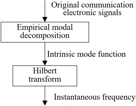
Drawing on the existing methods of time-frequency analysis, this paper introduces the Hilbert transform to the feature extraction and quantitative identification of signal features, in the light of the non-steady features of communication countermeasure electronic signals. Figure 1 shows the flow of the time-frequency analysis of communication electronic signals. The specific steps of the analysis are as follows:
Figure 1. Flow of time-frequency analysis of communication electronic signals
Firstly, the original communication electronic signals are decomposed through empirical modal decomposition to obtain the intrinsic mode function (IMF) satisfying the requirements of Hilbert transform:
$a\left( e \right)=\sum\limits_{i=1}^{m}{IM{{F}_{i}}\left( e \right)+S\left( e \right)}$ (1)
The Hilbert time-frequency map is derived from the instantaneous frequency of each IMF. The empirical modal transform can adaptively decompose the overlapping communication countermeasure electronic signals into a series of IMFs in natural modal forms, according to the features of these signals. Then, the IMFs meeting the conditions are subjected to the Hilbert transform to obtain the time-frequency variation, instantaneous frequency, and instantaneous amplitude of each IMF. On this basis, the three-dimensional (3D) time-frequency spectrum is plotted. The empirical modal decomposition can be realized in the following steps:
Firstly, the local maximum and minimum of the original communication electronic signal (e) are found. The envelope is obtained through cubic spline interpolation. Further, the instantaneous mean n(e) of the signal is solved.
Then, the communication electronic signal f(e)=a(e)-n(e) after eliminating the low frequencies is obtained by subtracting n(e) from a(e).
If the number of extremes and zero crossing points of f(e) are equal or have a difference of 1, and if the mean envelope determined by local maximums and minimums equals zero, then f(e) is an IMF. Otherwise, f(e) is the original communication electronic signal.
Repeating the above steps, the number of extremes and zero crossing points can be obtained. The first intrinsic modal component for the envelope to meet the above two conditions is denoted as d1(e).
Then, s1(e)=a(e)-d1(e) is obtained by subtracting a(e) from d1(e). Taking s1(e) as a new communication electronic signal, the above steps are implemented. The second component of the IMF thus obtained is denoted as d2(e). The third component of the IMF is denoted by d3(e).
After the above steps are implemented for m rounds, the residual term sm(e) is monotonous or constant, i.e., no new IMF component can be obtained. Then, the algorithm is terminated. Whether the algorithm is ended is judged by the standard deviation between two consecutive f(e):
$RC=\sum\limits_{i=0}^{E}{\frac{{{\left[ {{f}_{l-1}}\left( e \right)-{{f}_{l}}\left( e \right) \right]}^{2}}}{f_{l-1}^{2}\left( e \right)}}$ (2)
Let sm(e) be the residual term after the decomposition; di(e) be the i-th IMF component. The original communication electronic signal is the sum of all components and the residual term. Then, we have:
$a\left( e \right)=\sum\limits_{i=1}^{m}{{{d}_{i}}\left( e \right)}+{{s}_{m}}\left( e \right)$ (3)
Suppose a total of E samples are collected. Then, the energy of the communication electronic signal can be calculated by:
$T\left( i \right)=\sum\limits_{i=1}^{E}{{{d}_{i}}\left( e \right)}$ (4)
The Hilbert transform only changes the frequency spectrum of the communication electronic signal, without affecting the and other features of the signal. To obtain the instantaneous frequency of the communication electronic signal, it is necessary to find the amplitude and phase of the signal of each intrinsic modal component of the signal after the Hilbert transform, and then solve the derivative of signal phase relative to time.
The communication electronic signal can be parsed by:
${{c}_{i}}\left( e \right)={{d}_{i}}\left( e \right)+j{{\hat{d}}_{i}}\left( e \right)={{x}_{i}}\left( e \right){{t}^{j{{\varphi }_{j}}\left( e \right)}}$ (5)
The amplitude and phase of the signal can be given by:
${{x}_{i}}\left( e \right)=\sqrt{{{d}_{i}}{{\left( e \right)}^{2}}+{{{\hat{d}}}_{i}}{{\left( e \right)}^{2}}}$ (6)
${{\varepsilon }_{i}}\left( e \right)=arctan\frac{{{{\hat{d}}}_{i}}\left( e \right)}{{{d}_{i}}\left( e \right)}$ (7)
The instantaneous frequency of the IMF can be calculated by:
${{g}_{i}}\left( e \right)=\frac{1}{2\pi }{{\theta }_{i}}\left( e \right)=\frac{1}{2\pi }\frac{c\varphi \left( e \right)}{de}$ (8)
The instantaneous frequency of the communication electronic signal can be calculated by:
$a\left( e \right)=RP\sum\limits_{i=1}^{M}{\beta \left( e \right){{t}^{\varepsilon \left( e \right)}}}=RP\sum\limits_{i=1}^{M}{\beta \left( e \right){{t}^{j\int{\theta \left( e \right)}de}}}$ (9)
The Hilbert spectrum can be mathematically expressed as:
$F\left( \theta ,e \right)=RP\sum\limits_{i=1}^{M}{{{x}_{i}}\left( e \right){{t}^{j\int{\theta \left( e \right)}de}}}$ (10)
To obtain the Hilbert marginal spectrum, the time-domain integration of the Hilbert spectrum can be solved by:
$f\left( \theta \right)=\int_{0}^{E}{F\left( \theta ,e \right)de}$ (11)
To obtain the instantaneous energy density of the Electronic Signals, the frequency-domain integration of the square of the Hilbert spectrum amplitude can be solved by:
$ZQ\left( e \right)={{\int\limits_{\theta }{F\left( \theta ,e \right)}}^{2}}de$ (12)
Each high-density communication countermeasure electronic signal can be regarded as a densely superimposed pulse series of communication countermeasure radiation sources. The purpose of type identification of communication electronic signals is to separate the chronological pulse series, and to extract the characteristic parameters of each communication countermeasure radiation source. This paper modifies the PRI transform, a typical PRF type identification algorithm, and applies the modified approach to the type identification of communication electronic signals. Figure 2 illustrates the type identification of high-density communication countermeasure electronic signals.
Figure 2. Type identification of high-density communication countermeasure electronic signals
The PRI transform applies to jitter-free communication electronic signals. If the target communication electronic signal is a pulse series with random jitters. Let σm be the variation range of adjacent pulse intervals relative to O; o be the central value of the PRI. Then, the arrival time of each pulse in the series can be expressed as:
$\left\{ \begin{align} & {{e}_{0}}=0 \\ & {{e}_{m}}={{e}_{m-1}}+o\left( 1+{{\sigma }_{m}} \right),m=1,2,...,M-1 \\ \end{align} \right.$ (13)
Let σm be an independent identically distributed variable with the mean of zero and variance of ξ2. After the PRI transform, the phase of adjacent pulses can be expressed as:
$\begin{align} & \phi =2\pi {{e}_{m}}/\left( {{e}_{m}}-{{e}_{m-1}} \right)=2\pi \left( m+{{\sigma }_{1}}+...+{{\sigma }_{m}} \right)/\left( 1+{{\sigma }_{m}} \right) \\ & =2\pi \left( m+{{\sigma }_{1}}+...+{{\sigma }_{m}}-m{{\sigma }_{m}} \right)/\left( 1+{{\sigma }_{m}} \right) \\ & \approx 2\pi \left( {{\sigma }_{1}}+...+{{\sigma }_{m}}-m{{\sigma }_{m}} \right) \\ \end{align}$ (14)
When m is relatively great, σ1+...+σm-mσm is negatively correlated with m1/2, while mσm is proportional to m. Then, the phase of adjacent pulses can be estimated by:
${{\phi }_{m}}\approx -2\pi m{{\sigma }_{m}}$ (15)
The above modification of the PRI transform can overcome the defects of the traditional algorithm. The flow of the modified algorithm can be expressed as:
Step 1. Let Cl=0, 1≤l≤L, m=2, n=m-1, and ρ=em-en. If ρ≤(1-σ)ρmin, jump to Step 7; if ρ≥(1-σ)ρmin, jump to Step 8.
Step 2. Calculate the range of the PRI, and solve the width as yl=2σρl. Denote the upper and lower limits of the l-th PRI as ρl_low=(1-σ)ρl and ρl_high=(1+σ)σ, respectively. Choose all O values that satisfy ρO_low<ρ<ρO_high.
Step 3. Let l=o(1):o(end), and execute Steps 4-6.
Step 4. If the l-th PRI is being used for the first time, then set pl=em. Compute the initial phase, and solve δ0=(em-pl)/ρl, u=(δ0+0.5), and Φ=δ0/u-1.
Step 5. If either condition (1) or (2) is satisfied, set pl=em.
(1) u=1, and en=pl
(2) u≥2, and |Φ|≤Φ0
Step 6. Calculate δ=(e0-pl)/ρl and Cl=Cl+ exp(2πiδ).
Step 7. Let n=n-1. If n<1, jump to Step 8; otherwise, jump to Step 1.
Figure 3. Basic components of the type identification system of communication electronic signals
Step 8. Let m=m+1. If m>M, terminate the algorithm; otherwise, jump to Step 1.
The accurate PRI detection can be realized by properly setting the detection threshold. As shown in Figure 3, prior to type identification, the threshold for PRI detection can be determined based on the observation time, or based on the principle of eliminating harmonics and noises.
For a given communication electronic signal, the number of pulses with a PRI of ρl is denoted as |C(l)|, and the number of pulses that should appear in the observation time E is denoted as E/ρl; the adjustability coefficient is denoted as β. In the ideal state, there exists |C(l)|=E/ρl. Considering the pulse loss of the communication electronic signal, we have:
$\left| C\left( l \right) \right|\ge \beta \frac{E}{{{\rho }_{l}}}$ (16)
Let Dl be the number of pulses in the presence of harmonics. Then, |C(l)|<Dl. Let γ be the adjustability coefficient. Then, whether ρl is a PRI or a sub-harmonic can be judged by:
$\left| C\left( l \right) \right|\ge \gamma {{D}_{l}}$ (17)
Let |C(l)| be the noisy component of the original PRI. Then, the variance of |C(l)| should be smaller than Eτ2yl. Let τ be the pulse density of the communication electronic signal; yl be the width of the box; α be the adjustable parameter. Then, whether the component is a noise within the range of the PRI can be judged by:
$\left| C\left( l \right) \right|\ge \alpha \sqrt{E{{\tau }^{2}}{{y}_{l}}}$ (18)
Through the above analysis, the following threshold can be configured for PRI detection:
${{X}_{l}}=max\left\{ \beta \frac{E}{{{\rho }_{l}}},\gamma {{D}_{l}},\alpha \sqrt{E{{\tau }^{2}}{{y}_{l}}} \right\}$ (19)
Table 1 shows the communication distances measured by time-frequency analysis of high-density communication countermeasure electronic signals. It can be seen that the maximum and minimum absolute errors of the distance measured through the time-frequency analysis after Hilbert transform were 0.09mm and 0.01mm, respectively; the corresponding maximum and minimum relative errors were 0.4% and 0.014%, respectively.
Figures 4 and 5 compare the absolute and relative errors of different time-frequency analysis approaches, respectively. Our time-frequency analysis approach was compared with three reference methods: wavelet transform, Wigner-Ville distribution, and Choi-Williams distribution (CWD). It can be seen that our approach, which measures the communication distance through Hilbert time-frequency domain transform, had the smallest gap between measured distance and actual distance.
Table 1. Distance measurements of time-frequency analysis
|
Actual communication distance (mm) |
10 |
20 |
30 |
40 |
50 |
60 |
70 |
80 |
|
Measured communication distance (mm) |
10.04 |
20.07 |
30.05 |
40.02 |
50.05 |
60.09 |
70.01 |
80.03 |
|
Absolute error (mm) |
0.04 |
0.07 |
0.05 |
0.02 |
0.05 |
0.09 |
0.01 |
0.03 |
|
Relative error (%) |
0.4% |
0.35% |
0.167% |
0.05% |
0.1% |
0.15% |
0.014% |
0.037% |
Figure 4. Absolute errors of different time-frequency analysis approaches
Figure 5. Relative errors of different time-frequency analysis approaches
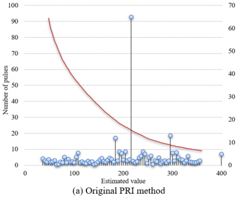
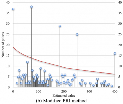
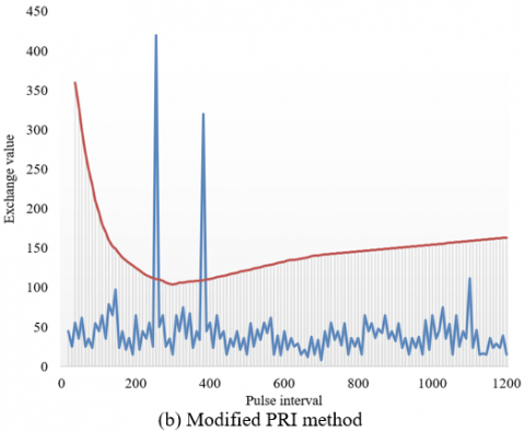
Figure 6. Results of original and modified PRI methods
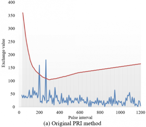
Figure 7. Simulation results at different jitter amounts
Figure 6 presents the experimental results of original and modified PRI methods. Concerning the third-order difference histogram, the original PRI transform could estimate a column of pulses. The original algorithm requires histogram accumulation, which is not necessary for the modified algorithm. Thus, the original algorithm incurs a heavier computing load than the modified one. The modified algorithm reduces the computing load, because it only compares the histogram of the current order with the detection threshold. However, when the degree of order of the difference histogram increases, the high-density communication countermeasure electronic signals would face a serious harmonic disturbance.
Figure 7 shows the simulation results at different jitter amounts. The modified PRI transform applies to the pulse series of high-density communication countermeasure electronic signals with jittering PRF, but does not apply to those with irregular PRF. Thus, the pulse series of high-density communication countermeasure electronic signals with irregular PRF were subjected to type identification tests. The modified PRI transform was applied to detect the pulse series of high-density communication countermeasure electronic signals with a fixed PRF, and those with jittering PRF. Based on the detected PRI, the pulse series were extracted from the original high-density communication countermeasure electronic signals, and the irregularity of the extracted signals were determined. Whether the modified algorithm is suitable for type identification was judge based on the number of residual signals.
This paper studies the time-frequency analysis and type identification of high-density communication countermeasure electronic signals. Both time and frequency domains were considered to analyze the signals, aiming to extract the time-frequency features of the signals more accurately. In this way, the authors captured the variation of non-stationary communication electronic signals in both time and frequency domains. Then, the PRI transform, a typical PRF type identification algorithm, was revised, before being introduced to the type identification of communication electronic signals. Then, the authors drew the flow chart of type identification of high-density communication countermeasure electronic signals. Through experiments, the communication distance was measured through the time-frequency analysis of high-density communication countermeasure electronic signals, and the absolute and relative errors of different time-frequency analysis methods were compared. The comparison shows that: our approach, which measures the communication distance through Hilbert time-frequency domain transform, had the smallest gap between measured distance and actual distance. Finally, the experiment results of original and modified PRI transforms were obtained, and the simulation results with different jitter amounts were displayed, revealing the effectiveness of the proposed PRI transform.
[1] Zhao, S., Liu, Z. (2021). Deception electronic counter‐countermeasure applicable to multiple jammer sources in distributed multiple‐radar system. IET Radar, Sonar & Navigation, 15(11): 1483-1493. https://doi.org/10.1049/rsn2.12140
[2] Luo, Y., Feng, C., Xia, Q., Ning, X. (2021). Study on the jamming-position maneuver algorithm of off-board active electronic countermeasure unmanned surface vehicles. IEEE Access, 9: 61184-61192. https://doi.org/10.1109/ACCESS.2021.3063856
[3] Tong, X.R. (2020). Modeling and realization of real time electronic countermeasure simulation system based on SystemVue. Defence Technology, 16(2): 470-486. https://doi.org/10.1016/j.dt.2019.08.010
[4] Kinugawa, M., Fujimoto, D., Hayashi, Y.I. (2019). electromagnetic information extortion from electronic devices using interceptor and its countermeasure. IACR Transactions on Cryptographic Hardware and Embedded Systems, 2019(4): 62–90. https://doi.org/10.13154/tches.v2019.i4.62-90
[5] Wei, Y., Gan, Y., Chen, Y., et al. (2018). A 50-W broadband mini-MPM for electronic countermeasure. IEEE Transactions on Electron Devices, 65(6): 2206-2211. https://doi.org/10.1109/TED.2018.2791723
[6] Kozlenko, M., Vialkova, V. (2020). Software defined demodulation of multiple frequency shift keying with dense neural network for weak signal communications. In 2020 IEEE 15th International Conference on Advanced Trends in Radioelectronics, Telecommunications and Computer Engineering (TCSET), Lviv-Slavske, Ukraine, pp. 590-595. https://doi.org/10.1109/TCSET49122.2020.235501
[7] Fang, W.J., Huang, X.G. (2013). Transmission of multibands wired and wireless orthogonal frequency division multiplexing signals using a full-duplex dense wavelength division multiplexing radio-over-fiber system. Optical Engineering, 52(1): 015003. https://doi.org/10.1117/1.OE.52.1.015003
[8] Smutzer, C.M., Techentin, R.W., Degerstrom, M.J., et al. (2012). A zero sum signaling method for high speed, dense parallel bus communications. In DesignCon 2012: Where Chipheads Connect, Santa Clara, CA, United States, pp. 896-919.
[9] Ramírez-Mireles, F. (2002). Signal design for ultra-wide-band communications in dense multipath. IEEE Transactions on Vehicular Technology, 51(6): 1517-1521. https://doi.org/10.1109/TVT.2002.804838
[10] Khoshouei, M., Bagherpour, R., Jalalian, M.H. (2021). Rock type identification using analysis of the acoustic signal frequency contents propagated while drilling operation. Geotechnical and Geological Engineering, 40: 1237-1250. https://doi.org/10.1007/s10706-021-01957-y
[11] Urbanavičiūtė, R., Petrolis, R., Tamašauskas, A., Skiriutė, D., Kriščiukaitis, A. (2021). Advanced image analysis-based evaluation of protein antibody microarray chemiluminescence signal improves glioma type identification by blood serum proteins concentrations. Computer Methods and Programs in Biomedicine, 211: 106416. https://doi.org/10.1016/j.cmpb.2021.106416
[12] Li, X., Fu, D., Mou, W., Liu, W., Wang, F. (2020). An identification method of navigation signal interference type based on SqueezeNet model. In 2020 IEEE 9th Joint International Information Technology and Artificial Intelligence Conference (ITAIC), Chongqing, China, pp. 875-880. https://doi.org/10.1109/ITAIC49862.2020.9338895
[13] Tian, H., Yin, L., Yang, X., Li, S., Yu, H. (2019). Wireless Signal Service Type Identification Based on Convolutional Neural Network. In 2019 IEEE 2nd International Conference on Electronic Information and Communication Technology (ICEICT), Harbin, China, pp. 748-753. https://doi.org/10.1109/ICEICT.2019.8846371
[14] Li, S., Zhao, D., Wang, X. (2019). Identification of transformer winding deformation fault type based on signal distance and SVM. In 2019 22nd International Conference on Electrical Machines and Systems (ICEMS), Harbin, China, pp. 1-6. https://doi.org/10.1109/ICEMS.2019.8922271
[15] Zhong, Y., Hao, J., Liao, R., Wang, X., Jiang, X., Wang, F. (2021). Mechanical defect identification for gas-insulated switchgear equipment based on time-frequency vibration signal analysis. High Voltage, 6(3): 531-542. https://doi.org/10.1049/hve2.12056
[16] Liu, Z. (2019). Time-frequency analysis and identification method for weak magnetic signal of submarine in aeromagnetic detection. In IOP Conference Series: Earth and Environmental Science, 310(2): 022046. https://doi.org/10.1088/1755-1315/310/2/022046
[17] Lei, M., Wei, Y., Li, Y., Wang, L. (2018). Sparse multi-wavelet-based identification of time-varying system with applications to EEG signal time-frequency analysis. Journal of Beijing University of Aeronautics and Astronautics, 44(6): 1312-1320.
[18] Cheng, P., Chen, Z., Li, Q., Gong, Q., Zhu, J., Liang, Y. (2020). Atrial fibrillation identification with PPG signals using a combination of time-frequency analysis and deep learning. IEEE Access, 8: 172692-172706. https://doi.org/10.1109/ACCESS.2020.3025374
[19] Luo, H., Ma, X.Y., Yang, H.G., Zhao, J.S., Xu, R. (2022). Measurement and analysis of dense frequency signal in power system. Zhongguo Dianji Gongcheng Xuebao/Proceedings of the Chinese Society of Electrical Engineering, 42(3): 929-941.
[20] Xing, K., Hao, K., Li, M. (2017). A new approach to dense spectrum analysis of infrasonic signals. In International Conference of Pioneering Computer Scientists, Engineers and Educators, Changsha, China, pp. 134-143. https://doi.org/10.1007/978-981-10-6385-5_12
[21] Zhao, X.D., Cheng, X.T., Zhang, Z.Y. (2011). The dense signal identification based on inner product and iteration. In 2011 International Conference on Electric Information and Control Engineering, Wuhan, China, pp. 4583-4586. https://doi.org/10.1109/ICEICE.2011.5777113
[22] Meng, Q., Chen, X., Zhu, Y., Hu, D., Li, R., Jiang, Y. (2019, November). Communication signal classification and recognition method based on GA-LSSVM classifier. In Journal of Physics: Conference Series, 1345(2): 022066. https://doi.org/10.1088/1742-6596/1345/2/022066
[23] Yuan, Y., Mei, W.B. (2005). Modulation recognition of communication signals based on time-frequency domain features and hierarchical decision classifier. Systems Engineering and Electronics, 27(6): 991-994.