Hamdullah Tung | Ramazan Tekin*
© 2022 IIETA. This article is published by IIETA and is licensed under the CC BY 4.0 license (http://creativecommons.org/licenses/by/4.0/).
OPEN ACCESS
The act of speaking takes place as a result of the joint use of both the senses of vision and hearing. The visual senses of the event of speech play an important role in lip-reading, especially when the sound is distorted or inaccessible. Visual-only-based lip-reading is a more difficult problem than audio-image-based lip-reading problems. In this study, three new spatial feature approaches to visual-only lip-reading are presented. To test the proposed feature extraction approaches, three datasets named AVLetters2 consisting of letters, AVDigits consisting of digits, and AVLetAVDig consisting of a combination of these two were used. First of all, the facial elements and lips were separated and the lip borders were marked with 20 points. Then, based on these spatial points, feature vectors were obtained with the feature approaches named Symmetric Euclidean Distance (SED), Central Euclidean Distance (CED), and Triple Points Angles (TPA). Extracted feature vectors were given to the CNN-LSTM network and 26 characters and 10 digits were tried to be estimated. As a result of the findings, the best success results for AVLetters2, AVDigits, and AVLetAVDig datasets were obtained by the SED+CNN+LSTM method as 53.2, 81.6, 59.8, respectively. When compared with the studies in the literature on the same data set, it was seen that very high and successful results were obtained.
lip reading, image processing, feature extraction, spatial features, deep learning
The act of speaking is not just an act of vocalization. It is a known fact for centuries that the speaker's facial movements contain useful information about speech [1]. During the speech, the shapes of the mouth can be observed with the eye, and thus lip reading can be performed. Lip-reading is a technique of understanding speech by analyzing the movement of lips, face, and tongue in situations where it is not possible to understand the sound. Therefore, lip-reading using only visual data emerges as a very important problem in cases where the voice is inaccessible or distorted or the perception functions are weakened in people with sensory loss due to various auditory disorders.
In lip-reading problems, the detection of the lip area is one of the most critical operations. Because all operations for lip-reading will be performed on this detected area, a possible error will directly affect the performance of the method. In early studies in this area, researchers often manually selected the lip area using lipstick or reflectors painted lip. With the developments in the field of face detection, the detection of lips has become possible thanks to various algorithms in computer systems. For example, in the study by Rao and Mersereau [2], the lip edge was extracted using the distinctive horizontal edge properties. However, this method is affected by light, shadow, and beard. Liévin and Luthon [3] used the color differences between skin and lips. Jun and Hua [4] used an adaptive lip detection algorithm based on chromaticity contrast. In this method, they used the HSV (Hue, Saturation, Value) color model to separate color and luminance. The method called Ensemble of Regression Trees, proposed by Kazemi and Sullivan [5], which was also used in this study, can locate landmark points by detecting faces and lips with HOG features combined with a linear-SVM classifier.
Extracting the features of the detected lip area after the lip borders determination is an important part of the lip-reading process by using the localized area. Effective and robust characteristic values directly affect lip reading/recognition performance. Zhang et al. [6] applied the Expectation-Maximization and Principal Component Analysis methods to the lip region to reduce the calculations. Morade and Patnaik [7] used the feature extraction method based on Discrete Wavelet Transform (DWT) and Large-Scale Detection Through Adaptation (LSDA). DWT was used only to extract visual information about the prominent speakers from the lip part. LSDA was used to reduce the feature size. Kawasaki et al. [8] applied two adaptations, speaker and environmental, to increase lip-reading performance. They stated that these two adaptations greatly increased lip-reading performance. Lee [9] used a temporal filtering technique called visual-speech pass filtering, which is used to extract visual features for automatic lip-reading. Lee used this filter to remove unwanted pixels around the speaker's lip and increase lip-reading performance. On the other hand, Kang et al. [10] extracted the facial movement features of the persons using a system that captures 3D facial movement features. The Hidden Markov Model and Viterbi algorithm were used for learning and recognizing each syllable.
Lip-reading applications offer solutions that can improve the ability of people with hearing impairment to learn or understand normal language expressions. Studies on this subject include many fields such as artificial intelligence, information engineering, and image processing systems. With the rapid developments in automatic speech recognition, human-computer interaction, and computer vision technologies, lip-reading applications are used not only to improve speech recognition but also in new areas such as human-machine and anti-terrorism [11].
In this study, three new spatial feature approaches to visual-only lip-reading are presented. To test the proposed feature extraction approaches, three datasets named AVLetters2 consisting of letters, AVDigits consisting of digits, and AVLetAVDig consisting of a combination of these two were used. The borders of the face and then the lip area of the speaker in each frame in these video images were determined and used to obtain the spatial landmark attributes placed on these borders. The deep learning method CNN-LSTM, which has Convolutional Neural Network (CNN) and LSTM layers, was used as the classifier method. As a result of the findings, the best success results for AVLetters2, AVDigits, and AVLetAVDig datasets were obtained by the SED+CNN+LSTM method as 53.2, 81.6, 59.8, respectively. The results obtained were also compared with the literature and it was seen that more successful results were obtained from the literature.
The following sections of this study are organized as follows. In the next section, literature studies on visual-only lip-reading are summarized. Section 3 provides details on the datasets used in this study. In Chapter 4, the proposed feature extraction methods and classification model are described. In Chapter 5, the obtained experimental results are analyzed and discussed in detail. In the last section, the important results of the study are stated.
Frisky et al. [12] performed a study based on visual lip movement recognition by applying the video content analysis technique. In the study, they proposed a new visual-only speech recognition method using Non-Negative Matrix Factorization and Kernel Sparse Representation Classifier (K-SRC). In this study, they extracted Local Binary Patterns (LBP) based features over Three Orthogonal Planes (TOP) by using Spatio-temporal feature descriptors related to both space and time from videos containing visual lip information. They used AVLetters and AVLetters2 datasets to measure the performance of their proposed method.
Tian and Ji [13] conducted a study using the Auxiliary multimodal Long Short-Term Memory (Am-LSTM) method, which is an artificial recurrent neural network architecture used in the field of deep learning for Audio-visual Speech Recognition (AVSR). LSTM is a Recurrent Neural Network architecture designed to deal with long-term dependencies [14]. Unlike standard feedforward neural networks, LSTM has feedback connections [15]. It can process not only single data points but also entire data series. In this study, they performed an AVSR application using both video and audio data. For this purpose, the proposed method in the study was applied to 3 different data sets, namely AVLetters, AVLetters2, and AVDigits.
Bear et al. [16] developed a phoneme-clustering model for speaker-dependent and speaker-independent phoneme-to-viseme mapping. These maps were used to reveal how the speech patterns are visually similar. The speakers' faces were tracked using Active Appearance Models (AAM), in which only lip-combined shape and appearance features were extracted.
Mattos et al. [17] studied visual recognition improvement based on Convolutional Neural Networks using synthetic data. In this study, the problem of recognizing visemes, which are the visual equivalents of phonemes, is discussed. They solved this problem by creating a large-scale synthetic 2D dataset based on realistic 3D face models that were automatically labeled. In these studies, datasets named AVDigits, AVLetters, Cuave, and GRID corpus were used.
Fernandez-Lopez and Sukno [18], on the other hand, carried out a very comprehensive study in terms of both the applied methods and the datasets related to automatic lip-reading in their studies using deep learning. In this study, researches in the field of automatic lip-reading in recent years are reviewed, and both previous approaches called traditional and recent developments in automatic lip-reading architectures are discussed. They considered many very large datasets such as words and phrases.
In this study, three new spatial feature approaches to visual-only lip-reading are presented. To test the proposed feature extraction approaches were used aligned audio-visual data consisting of isolated letters named AVletters2 and isolated digits named AVDigits. The AVletters2 dataset is an extension of the AVLetters [1] dataset created by Cox et al. [19]. This dataset contains 26 letters from the letter "A" to the letter "Z" sung by five people, with seven repetitions for each letter. AVDigits, on the other hand, were created by Hu and Li [20] and contain records of each of the 10 digits between 0 and 9 being repeated 9 times by 6 people. Detailed information about both data sets is presented in Table 1 below.
Table 1. Details on datasets
|
|
AVLetters2 |
AVDigits |
|
Video Recording content |
Letters between 'A' and 'Z' |
digits from '0' to '9' |
|
Number of Classes |
26 |
10 |
|
Number of Speakers |
5 |
6 |
|
Number of repetitions |
7 |
9 |
|
Number of pronunciations |
910 |
540 |
|
Frame Size |
1920 × 1080 |
1920 × 1080 |
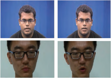
Figure 1. Sample images of speakers in the AVLetter2 and AVDigits datasets
Audio and video contents in the dataset are divided into raw data. The images in this dataset were recorded in color using 1920*1080 RGB with high-definition cameras [21]. Example images of some speakers in the AVletters2 and AVDigits datasets are shown in Figure 1.
4.1 Lip-reading system scheme
Lip-reading applications consist of various calculation processes. Therefore, by dividing the system into sections at various levels, evaluating the operations to be performed in each section separately defines the whole system better. The proposed system scheme for lip-reading within the scope of this study is shown in Figure 2. The proposed system consists of 4 stages. The procedures performed at each stage are summarized below.
Stage 1: In each frame of the video images, the detection of the face and other elements on the face ((lip, eye, eyebrow, etc.) is realized at this stage. Since the data processed at this stage is video, a 3-dimensional matrix is produced, consisting of the image of the lip region cross-section, in the number of frames for each element.
Stage 2: In the next stage, the marker points on the lip are determined from the regionally determined lip contours. At this stage, the inner and outer lip borders determined in each frame are marked with a total of 20 points. The data produced at this stage is a 2-dimensional matrix containing 20 marker points for each frame.
Stage 3: At this stage, spatial information is calculated with three different proposed feature extraction methods using landmark points, and appropriate feature vectors are created for the classification methods. The data produced at this stage is a 1-dimensional vector containing the distance or angular metric values obtained from 20 marker points for each frame.
Stage 4: At this stage, the classification process is carried out. By using the extracted features from stage 3, it is tried to predict the pronounced letter or number with the CNN-LSTM classification method, which is a deep learning method that is a combination of Convolutional Neural Network and LSTM.
All operations were performed on a personal computer with AMD Ryzen 7 5800H processor and 16 GB RAM. Face detection from video images, detection of lip markings, feature extraction, and classification processes are all performed using Python programming language and DLib [22] and OpenCV libraries. TensorFlow Keras framework was used for the implementation of deep learning methods [23].
4.2 Detection of lip points
To detect lip points, first of all, the face and then lips must be detected. Dlib face landmark detector and OpenCV python libraries were used to detect face and lips. Dlib is an open-source library aimed at both engineers and scientists, aiming to provide a C++ environment [22]. Applications such as face recognition, face detection, and facial landmarks can be obtained through the dlib library.
Detection of facial points requires an important step, such as detecting the face and facial regions in the image. For face detection, methods such as the Haar-cascade algorithm [24], Viola and Jones detector [25] or Histogram of Oriented Gradients [26], or deep learning-based algorithms can be used. The important thing here is to determine the borders that limit the face. In the second stage, it is necessary to mark the items on the face. There are various marker algorithms developed for this purpose. These algorithms mostly mark items such as mouth, right and left eyebrows, right and left eyes, nose, and chin. The most important element for us in this study is the mouth area. Because it is thought that the lip area takes various forms during the pronunciation of the letters and this varies for each letter. Therefore, during the pronunciation of the letters/digits, the spatial coordinates of the markers showing the mouth boundaries in each video frame change relative to each other, which can provide us with very useful features in classifying the letters/digits. For this purpose, in this study, the method called Ensemble of Regression Trees, proposed by Kazemi and Sullivan [5], was used to detect the points on the lip borders after face detection with HOG features combined with a linear-DVM classifier. In this method, a cascade/stepwise multiple regression structure was used. Details of the method proposed by Kazemi and Sullivan [5] are given below.
In the Ensemble of Regression Trees (ERT) method, a training dataset is used in which the face elements are labeled manually (by marking the (x,y) coordinates). Then, an ERT is trained on based pixel intensities to detect facial markings by using a trained dataset. Each regressor rt (∙,∙) in the cascade structure further improves the prediction by adding the update vector obtained from the I image and the current prediction $\hat{S}^{(t)}$ to the current prediction $\hat{S}^{(t)}$ [5]:
$\hat{S}^{(t+1)}=\hat{S}^{(t)}+r_{t}\left(I, \hat{S}^{(t)}\right)$ (1)
where, $x_{i}$specifies the (x, y) coordinates of the face sign in image I. Accordingly, the coordinates of p face signs-in the I image are Accordingly, the coordinates of p face signs in the I image are $S=\left(\mathrm{x}_{1}^{T}, \mathrm{x}_{2}^{T}, \ldots, \mathrm{x}_{p}^{T}\right)^{T} \in \mathbb{R}^{2 p}$, with the current estimate of S with $\hat{S}^{(t)}$ is expressed.
The critical point in the cascade structure is that the $r_{t}$ regressor makes its predictions based on properties such as pixel intensity values calculated from I and indexed against the current shape estimate $\hat{S}^{(t)}$. This introduces a kind of geometric invariance to the process, and as the cascade progresses, one can be more certain that a precise semantic position on the face is indexed. In this method, to train each $r_{t}$ Hastie et al. As explained by Hastie et al. [27], the gradient tree boosting algorithm was used with a sum of squared error loss. Details about the method are explained in the study by Kazemi and Sullivan [5].
Figure 2. The steps used for lip reading
4.3 Spatial features
The spatial features proposed within the scope of this study were obtained by using 20 points detected above the lip in the frames in each video image, as seen in Figure 3(a) below. These features obtained from the frames in the video image containing the pronunciation recording were brought together to create a feature vector for each recording. There are a total of 910 and 540 video recordings in the AVLetters2 and AVDigits datasets, respectively. The number of frames of the videos differs from each other. In the AVLetters2 and AVDigits datasets, the highest frame counts were 67 and 64 frames, respectively, and the lengths of the feature vectors were made equal by repeating the last frame features of the records containing fewer frames.
The feature extraction approaches detailed below were obtained according to the spatial landmark points in Figure 3(a). There are a total of 20 points, 12 of which are on the outer lip $\left(P_{i}, i=1,2, \ldots, 12\right)$ and 8 on the inner $\left(P_{i}, i=13,14, \ldots, 20\right)$.
Symmetric Euclidean Distance (SED): In the SED feature extraction approach, as seen in Figure 3(b), the Euclidean-Distance (Eq. (2)) [28] between the upper and lower vertical symmetrical landmarks of the lip was calculated and the feature vector was obtained. In addition, the horizontal distance between the outer edge $\left(P_{1}\right.$ with $\left.P_{7}\right)$ and the inner edge $\left(P_{13}\right.$ with $\left.P_{17}\right)$ reference points is calculated and added to this feature vector. A total of 67 x 10=670 and 64 x 10=640 features were obtained for each video recording of the AVLetters2 and AVDigits datasets, respectively, 10 features for each frame, and these features were given to the classifier.
$d(i, j)=\sqrt{\sum_{k=1}^{p}\left(X_{i k}-X_{j k}\right)^{2}}$ (2)
where, $d(i, j)$ denotes the Euclidean distance between two points (points $X_{i}$ and $X_{j}$), each represented by the $p$ plane.
Central Euclidean Distance (CED): In the CED feature extraction approach, the spatial coordinates of the midpoint between the left outer edge ($P_{1}$) and the right outer edge ($P_{7}$) landmark points, which are marked with red in Figure 3(c), are obtained. Then, the Euclidean-Distance (Eq. (2)) between the other lip landmarks and this reference point was calculated and the feature vector was obtained. A total of 67 x 20=1340 and 64 x 20=1280 features were obtained for each video recording of AVLetters2 and AVDigits datasets, respectively, 20 features for each frame, and these features were given to the classifier.
Triple Points Angles (TPA): In the TPA feature approach, as seen in Figure 3(d), the angles formed between the 10 landmarks on the outer borders of the lip and the left outer edge ($P_{1}$) and the right outer edge ($P_{7}$) were calculated in radians according to Eq. (3) and the feature vector has been obtained. In addition, radial angles calculated between the left inner edge ($P_{13}$) and the right inner edge ($P_{17}$) with the 6 marker points located on the inner borders of the lip are added to this feature vector. A total of 67 x 16=1072 and 64 x 16=1024 features were obtained for each video recording of the AVLetters2 and AVDigits datasets, respectively, 16 features for each frame, and the obtained features were given to the classifier.
The third feature extraction approach proposed in this study, TPA, uses the radial angle measure between three points. The angle θ between the two vectors $(\overrightarrow{\boldsymbol{A B}}$ and $\overrightarrow{\boldsymbol{B C}})$ formed by the points A, B and C in Euclidean space can be calculated as follows,
$\theta \text{=co}{{\text{s}}^{-1}}(\frac{\overrightarrow{AB}\,\,\,\cdot \overrightarrow{BC}}{\left\| \overrightarrow{AB} \right\|\left\| \overrightarrow{BC} \right\|})$ (3)
where, $\longrightarrow$ denotes the Euclidean vector, $\|\rightarrow\|$ the length of the vector, and “∙” the inner product.
Figure 3. 20 points and features detected on the lip borders
Figure 4. CNN+LSTM deep learning structure (Conv1D:1D convolution layer, F: Filter, K: Kernel, BN: Batch normalization layer, MP-1D: 1D max pooling layer, Dout: Dropout, PS: Pool Size, Sout: Output Space, nC: Number of class)
4.4 CNN-LSTM
In this study, a deep learning method called CNN-LSTM, which uses Convolutional Neural Network (CNN) layers and combined with LSTM, is used to compare the performances of the proposed feature approaches. Although the CNN model has capabilities such as automatically obtaining features with convolution layers, its capabilities are limited in modeling data with a consecutiveness relationship. For this, LSTM networks with the ability to use previous dependencies can be used together with CNN. For this purpose, in this study, a deep learning network called CNN-LSTM, which can take into account the sequential changes of the landmark points detected on the lip in each frame during the pronunciation of letters or digits, was used. The structure of the CNN-LSTM architecture used in this study is shown in Figure 4.
As seen in Figure 4, there are various levels of 1D-Convolution, max pooling and fully connected layers in the architecture. Depending on the type of input data, various sizes of convolution operation can be applied. Kernel size is determined accordingly. In this study, 1-dimensional CNNs are used for convolution operations in the models, since feature vectors based on the distance and angle criteria of the lip landmarks obtained from the image are used. Various activation functions can be applied to add non-linearity to the CNN, LSTM and fully connected layers in the architecture presented in Figure 4. In our study, RELU (Rectified Linear Unit) function was applied in all layers. Softmax is used as the activation function in the output layer, which is the last layer in the architecture. In addition, number of Class (nC), which determine the output size of the last layer, are taken as 26 and 10, respectively, which are the class number values of AVLetters2 and AVDigits data sets.
4.4.1 Convolutional Neural Networks (CNN)
Convolutional Neural Networks (CNN) is a special type of multilayer perceptron based on Artificial Neural Networks (ANN). CNN, which is a widely used deep learning method and especially applied to images, provides automatic obtaining of features by applying various filters and convolution operations to the images. CNN can have convolutional, pooling and fully connected layers in varying numbers depending on the problem. In addition, after the convolutional layers, there may be pooling layers that reduce the computational cost by reducing the output data of these layers.
4.4.2 Long-Short Time Memory (LSTM)
Traditional ANNs cannot use the information from the previous step during modeling for the current step. Recurrent Neural Networks (RNN), which enables information to be remembered, offers a solution to this problem. They do this with feedback connections between hidden layers that act as internal memory. These layers process the input data sequentially, using a feature vector that preserves contextual information. Long-Short Time Memory (LSTM) is a special type of RNN that can learn short- and long-term dependencies. The LSTM network is trained using backpropagation in time and overcomes the problem of disappearing gradient in long-term dependencies in RNNs [29]. The general structure of an LSTM cell is presented in Figure 5.
While traditional neural networks have neurons, LSTM networks have memory blocks interconnected by cascading layers. Each block consists of four basic gates: the forget gate, which determines what information from the previous unit is to be forgotten, the input gate which decides what to accept into the neuron, the update gate which updates the cell, and finally the output gate, where new long-term memory is created. The basic mathematical expressions of these gates in the LSTM structure are presented below [30]:
$i_{t}=\sigma\left(W_{i} *\left[h_{t-1}, x_{t}\right]+b_{i}\right)$ (4)
$f_{t}=\sigma\left(W_{f} *\left[h_{t-1}, x_{t}\right]+b_{f}\right)$ (5)
$\tilde{c}_{t}=\tanh \left(W_{c} *\left[h_{t-1}, x_{t}\right]+b_{c}\right)$ (6)
$c_{t}=f_{t} * c_{t-1}+i_{t} * \tilde{c}_{t}$ (7)
$o_{t}=\sigma\left(W_{o} *\left[h_{t-1}, x_{t}\right]+b_{o}\right)$ (8)
$h_{t}=o_{t} * \tanh \left(c_{t}\right)$ (9)
where, $W_{x}$ and $b_{x}$ represent weight matrices and bias vectors ($x=i, f, t, o$), respectively. $f_{t}$ forget gate vector, $i_{t}$ input (update) gate vector, $o_{t}$ output gate vector, $x_{t}$ current input data, $h_{t-1}$ hidden state vector, $c_{t}$ current state vector, $\sigma(\cdot)$ sigmoid activation function, and the * operator the elementary product of the vectors.
Figure 5. General structure of the LSTM cell [30]
4.5 Performance metrics
Performance criteria such as Accuracy, Precision, Recall/Sensitivity, Specificity, and f-measure were used to reveal the performance of the approaches used in the study. The following expressions are used to calculate these performance criteria.
Accuracy $=\frac{T P+T N}{T P+T N+F P+F N}$
Precision $=\frac{T P}{T P+F P}$
Recall/Sensitivity $=\frac{T P}{T P+F N}$
$F-$ Measure $=2 \frac{\text { Recall } * \text { Precision }}{\text { Recall }+\text { Precision }}$ (10)
In these equations, T, F, P, and N represent the concepts of true, false, positive, and negative, respectively. For example, TP is the number of correctly classified positive samples; FN indicates the number of negative samples that were misclassified.
Accuracy: It is the most popular and simple method used to determine the accuracy of the model. This ratio is defined as the ratio of the number of correctly classified (TP+TN) samples to the total number of samples (TP+TN+FP+FN).
Precision: Measures how good the model is at predicting positive events. It is the ratio of the number of samples labeled as positive (TP) to the total samples classified as positive (TP+FP).
Recall/Sensitivity: It measures how well the model is suitable for detecting events in the positive class. It is the ratio of positively labeled samples (TP) to the total number of truly positive samples (TP+FN). Sensitivity is calculated similarly, measuring how well the model is at detecting positive events.
Specificity: It measures how accurate the model is in assigning the positive class. It is the ratio of negatively labeled samples (TN) to the total number of truly negative samples (TN+FP).
F-Measure: Precision and sensitivity (Recall) metrics are interrelated, and the two are combined to give the F-Measure, which is their harmonic mean. It is used to optimize the system towards precision or sensitivity.
For the AVLetters2 and AVDigits datasets used in the study, the partially speaker-dependent and completely speaker-independent results obtained by using 10 cross-validation results with the CNN-LSTM deep learning method are presented below. In the model, the RELU activation function and the dropout parameter value as 0.25 was chosen because it gave the best results. Epochs and batch size were selected as 5000 and 100, respectively. Cross validation was carried out in the form of stratified sampling. Stratified sampling is a sampling method used in situations where the dataset can be divided into subgroups and each subgroup sample needs to be represented during sampling, as in the problem here.
5.1 Partially speaker dependent results
There are 182 and 90 records for each user in the AVLetter2 (5 speakers) and AVDigits (6 speakers) datasets, respectively. Partially Speaker Dependent (PSD) applications were realized because the size of this data set did not contain enough data to evaluate each speaker separately for the deep learning model. In PSD lip-reading applications, the data set is divided into train and test sets as in speaker-independent applications. However, after the model was trained with the training dataset, only one speaker's data in the test dataset was selected and applications were carried out. The performance results obtained with the SED, CED, and TPA feature extraction approaches are given in Table 2 and Table 3.
As seen in Table 2, for the AVLetters2 dataset, the best method for $S_{1}$ and $S_{4}$ speakers was SED+CNN-LSTM, and 63.74% and 54.81% accuracy were obtained, respectively. For $S_{2}, S_{3}$, and $S_{5}$ speakers, the best method was CED+CNN-LSTM and accuracy values of 62.82%, 67.40%, and 52.41% were obtained, respectively.
In Table 3, speaker-dependent accuracy measures are presented according to the SED, CED and TPA feature extraction approaches proposed for 6 different speakers belonging to the AVDigits dataset.
Table 2. AVLetters2 PSD accuracy (%) with CNN-LSTM Model (Speakers $\mathrm{S}_{\mathrm{i}}, \mathrm{i}=1,2,3,4,5$)
|
Method |
$S_{1}$ |
$S_{2}$ |
$S_{3}$ |
$S_{4}$ |
$S_{5}$ |
|
SED |
63.74 |
59.34 |
66.65 |
54.81 |
49.81 |
|
CED |
49.41 |
62.82 |
67.40 |
46.64 |
52.41 |
|
TPA |
47.50 |
55.56 |
55.00 |
39.71 |
48.69 |
Table 3. AVDigits speaker dependent accuracy (%) with CNN-LSTM Model (Speakers $\mathrm{S}_{\mathrm{i}}, \mathrm{i}=1,2,3,4,5,6$)
|
Method |
$S_{1}$ |
$S_{2}$ |
$S_{3}$ |
$S_{4}$ |
$S_{5}$ |
$S_{6}$ |
|
SED |
89.49 |
82.23 |
87.09 |
89.17 |
93.36 |
78.36 |
|
CED |
87.50 |
77.50 |
71.07 |
92.50 |
92.50 |
84.17 |
|
TPA |
85.32 |
79.17 |
84.62 |
67.74 |
79.17 |
66.95 |
As seen in Table 3, for the AVDigits dataset, the best method for $S_{1}, S_{2}, S_{3}$ and $S_{5}$ speakers were SED+CNN-LSTM, and 89.49%, 82.23%, 87.09% and 93.36% accuracy were obtained, respectively. For $S_{4}$ and $S_{6}$ speakers, the best method was CED+CNN-LSTM and accuracy values of 92.50% and 84.17% were obtained, respectively.
5.2 Completely speaker independent results
Completely Speaker-Independent (CSI) applications were carried out on the datasets named AVLetter2 and AVDigits and the datasets named AVLetAVDig, which were created by combining them. In Table 4, the performance values obtained using the CNN-LSTM deep learning model with the proposed SED, CED, and TPA feature extraction approaches for AVLetter2, AVDigits and AVLetAVDig datasets are given.
Table 4. Completely speaker independent accuracies with CNN-LSTM model (%)
|
Data set |
Method |
Train Acc. (%) |
Test Acc. (%) |
Test Precision |
Test Recall |
Test F1-Score |
|
AVLetters |
SED |
100 |
59.62 |
0.63 |
0.60 |
0.59 |
|
CED |
100 |
54.81 |
0.57 |
0.55 |
0.54 |
|
|
TPA |
98.64 |
50.00 |
0.52 |
0.50 |
0.48 |
|
|
AVDigits |
SED |
100 |
86.67 |
0.89 |
0.87 |
0.86 |
|
CED |
100 |
85.00 |
0.87 |
0.85 |
0.85 |
|
|
TPA |
97.71 |
78.33 |
0.80 |
0.78 |
0.77 |
|
|
AVLetAVDig |
SED |
100 |
64.02 |
0.68 |
0.64 |
0.63 |
|
CED |
99.69 |
63.63 |
0.66 |
0.65 |
0.64 |
|
|
TPA |
94.48 |
57.93 |
0.63 |
0.58 |
0.58 |
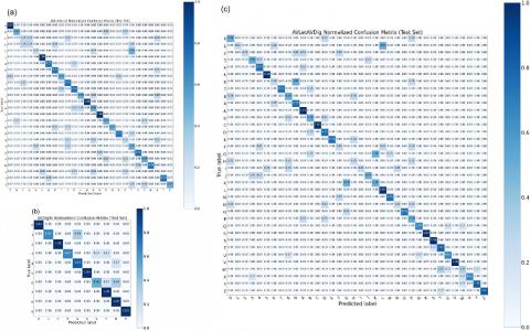
Figure 6. CSI best model confusion matrix for each dataset
As seen in Table 4, test accuracy values of AVLetter2, AVDigits, and AVLetAVDig datasets were found as 59.62%, 86.67%, and 64.02%, respectively. The best highest accuracies for all three datasets were obtained with SED+CNN-LSTM method. According to these results, it is seen that quite high accuracies have been achieved on the AVLetters2 and AVDigits dataset compared to the performances of the studies in the literature (discussed in the following sections). In Table 5 below, the averages of the accuracies obtained as a result of 10 cross-folds of the test data for all data sets are listed.
As seen in Table 5, CSI accuracy values of AVLetter2, AVDigits, and AVLetAVDig datasets were obtained as 53.2%, 81.6% and 59.8%, respectively. According to these results, it is seen that the most successful method for all three data sets is SED+CNN-LSTM.
Table 5. Average success rates for CSI with CNN-LSTM model (%)
|
Data sets |
Methods |
||
|
SED |
CED |
TPA |
|
|
AVLetters |
53.2 |
51.9 |
45.7 |
|
AVDigits |
81.6 |
79.7 |
72.9 |
|
AVLetAVDig |
59.8 |
57.8 |
52.8 |
Figure 6 (a,b,c) shows the confusion/complexity matrices of AVLetter2, AVDigits, and AVLetAVDig datasets, respectively. These matrices were created using the SED+CNN-LSTM model, which has the highest accuracy value according to the Test datasets.
In these matrices, normalized correct prediction rates $\left(R_{i, \text { Norm }}=X_{i, \text { True }} / X_{i}\right.$) are presented (diagonal values in the matrix) by dividing the number of correct predictions ($X_{i, T r u e}$) of each letter/digit by the total number of samples ($X_{i}$) of this letter/digit. The values other than the diagonal values in the confusion matrix show the false prediction rates.
Table 6. Success rates and directions of change
|
AVLetters2 |
AVDigits |
AVLetAVDig |
Direction of change |
|
|
0 |
- |
1.00 |
0.50 |
(-0.50) ↓ |
|
1 |
- |
0.67 |
0.25 |
(-0.42) ↓ |
|
2 |
- |
1.00 |
0.25 |
(-0.75) ↓ |
|
3 |
- |
0.67 |
0.50 |
(-0.17) ↓ |
|
4 |
- |
0.83 |
0.75 |
(-0.08) ↓ |
|
5 |
- |
1.00 |
1.00 |
(0.00) ↔ |
|
6 |
- |
0.50 |
0.25 |
(-0.25) ↓ |
|
7 |
- |
1.00 |
0.75 |
(-0.25) ↓ |
|
8 |
- |
1.00 |
0.50 |
(-0.50) ↓ |
|
9 |
- |
1.00 |
0.75 |
(-0.25) ↓ |
|
A |
1.00 |
- |
1.00 |
(0.00) ↔ |
|
B |
0.50 |
- |
0.50 |
(0.00) ↔ |
|
C |
0.25 |
- |
1.00 |
(+0.75) ↑ |
|
D |
0.25 |
- |
0.75 |
(+0.50) ↑ |
|
E |
0.25 |
- |
0.75 |
(+0.50) ↑ |
|
F |
1.00 |
- |
0.25 |
(-0.75) ↓ |
|
G |
0.75 |
- |
0.00 |
(-0.75) ↓ |
|
H |
0.75 |
- |
0.25 |
(-0.50) ↓ |
|
I |
0.50 |
- |
0.25 |
(-0.25) ↓ |
|
J |
0.75 |
- |
0.50 |
(-0.25) ↓ |
|
K |
0.75 |
- |
0.50 |
(-0.25) ↓ |
|
L |
0.50 |
- |
1.00 |
(+0.50) ↑ |
|
M |
1.00 |
- |
0.75 |
(-0.25) ↓ |
|
N |
0.50 |
- |
0.25 |
(-0.25) ↓ |
|
O |
1.00 |
- |
0.75 |
(-0.25) ↓ |
|
P |
0.50 |
- |
0.50 |
(0.00) ↔ |
|
Q |
0.50 |
- |
0.67 |
(+0.17) ↑ |
|
R |
0.75 |
- |
1.00 |
(+0.25) ↑ |
|
S |
0.25 |
- |
1.00 |
(+0.75) ↑ |
|
T |
0.50 |
- |
0.83 |
(+0.33) ↑ |
|
U |
0.75 |
- |
0.67 |
(-0.08) ↓ |
|
V |
0.50 |
- |
1.00 |
(+0.50) ↑ |
|
W |
0.75 |
- |
0.33 |
(-0.42) ↓ |
|
X |
0.00 |
- |
0.67 |
(+0.67) ↑ |
|
Y |
0.75 |
- |
0.83 |
(+0.08) ↑ |
|
Z |
0.50 |
- |
0.83 |
(+0.33) ↑ |
In Figure 6(a), it can be seen that the letters A, F M and O in the AVLetters2 dataset are predicted very accurately ($R_{i, \text { Norm }}=1.0$). It is seen that the letters G, H, J, K, R, U, W and Y are predicted correctly with a high rate ($R_{i, \text { Norm }}=0.75$), although they are relatively lower than the previous one. However, it is seen that the letter X cannot be predicted correctly and is confused with the letters S, N, K and F. In addition, it is seen that the letters C, D, E, and S are predicted with a low rate ($R_{i, \text { Norm }}=0.25$).
In Figure 6(b), it is seen that the digits 0, 2, 5, 7, 8 and 9 in the AVDigits data set are predicted correctly ($R_{i, \text { Norm }}=1.0$) with a very high rate. Although it is relatively lower than the previous one, it is seen that the digit 4 is also predicted correctly with a high rate ($R_{i, \text { Norm }}=0.83$). However, it is seen that the digit 6 is predicted with the lowest rate ($R_{i, \text { Norm }}=0.5$) and is mostly confused with the digits 8 and 7, respectively (according to the high false prediction rate). Finally, it is seen that the digits 1 and 3 are predicted correctly ($R_{i, N o r m}=0.67$) in a good ratio between the lowest and highest rates.
Figure 6(c) shows the normalized confusion matrix of letters and digits in the AVLetAVDig dataset created by combining AVLetters2 and AVDigits datasets. Accordingly, it is seen that the digit 5 and the letters A, C, L, R, S, and V are predicted very accurately. However, it is seen that the letter G cannot be predicted correctly and is confused with the letters K, B, and L. The lowest ($R_{i, \text { Norm }}=0.25$) predictions are seen to be 1, 2, 6 digits and the letters F, H, I and N according to AVLetters2 and AVDigits, respectively.
It was observed that combining different letter and digit groups, increased the accuracy of our proposed SED+CNN-LSTM model for the AVLetters2 dataset, but decreased the accuracy for the AVDigits dataset. For the AVLetAVDig dataset, the accuracy values of the AVLetters2 and AVDigits samples of our SED+CNN-LSTM model were found with 66.94% and 55.00%, respectively. According to the best model results in Table 4, accuracy value increased by 12.27% for AVLetters2, but decreased by 36.54% for AVDigits. This is expected for AVDigits. Because AVDigits, which consists of 10 classes, was combined with AVLetters2, which consists of 26 classes, and the number of classes was increased to 36. In the AVLetters2 dataset, the number of classes increased from 26 to 36, however, as the number of samples in the dataset increased, the training dataset of the model increased and it is seen that the model's success increased by training the model better.
Table 6 lists the correct prediction rates of the AVLetters2 and AVDigits datasets and the AVLetAVDig dataset created by combining them, according to the confusion matrices in Figure 6. In addition, the changes in accuracy rates according to the dataset AVLetAVDig combined with AVLetters2 and AVDigits datasets and the directions of these changes are presented in the table. The first 10 rows of the table belong to the digits in the AVDigits dataset, and almost all of them (except the digit 5) show a decrease in correct prediction rates. This is due to the increase in the number of classes from 10 to 36 in the combined data set, as stated before. Except for the first 10 lines, the other 26 lines belong to the letters in the AVLetters2 dataset. There was an upward change in 12 of these letters, a downward change in 11, and no change in the other 3 letters. It is seen that the number of letters whose accuracy change rates change up and down are almost equal. However, the reason for the increase in overall accuracy is that the sum of those whose rates of change are changing upwards is greater than the sum of those that are changing downwards. Change values are given in parentheses in the “Direction of Change” column in Table 6. The sign of the change values also indicates the direction of the change (down (↓) and + up (↑)). The sum of these accuracy values was +1.33 (↑) for AVLetters2 letters, while it was -3.17 (↓) for AVDigits digits. Accordingly, accuracy increased for AVLetters2 and decreased for AVDigits in the combined dataset.
As a result of this study, it can be said that the reason why some letters/digits are misclassified is due to the similarity of lip movements during pronunciation, and therefore the model confuses the letters. Since the lip movements during the pronunciation of these sounds are similar, the spatial features obtained are also almost similar. This causes decreasing of the classification accuracy of the model. However, when compared the successful results of this study with the existing studies in the literature, it is seen that the proposed feature extraction methods are quite successful in visual-only lip-reading applications. In the next section, the feature extraction approaches proposed in this study and the results obtained by the CNN-LSTM deep learning method used are compared with the results obtained in previous studies. In the next section, the results obtained with the CNN-LSTM deep learning model using the feature extraction approaches proposed in this study are compared with the studies in the literature.
5.3 Comparison of results
The comparison of the 10 cross-fold accuracy averages of the visual-only lip-reading applications obtained by using the proposed spatial feature approaches with the existing studies are presented in tables below. Comparisons between the results of completely speaker-independent studies in the literature on the AVLetters2 dataset and the results of the approaches proposed in this study are presented in Table 7.
Table 7. AVLetters2 CSI accuracy (%) comparisons
|
Study |
Features |
Classifier |
Accuracy (%) |
|
[19] |
AAM |
HMM |
8.3 |
|
[12] |
LBP-TOP |
K-SRC |
25.90 |
|
[12] |
LBP-TOP |
K-SRC |
24.2 |
|
[20] |
RTMRBM |
31.21 |
|
|
[31] |
raw-ROI |
B-LSTM |
42.6 |
|
[31] |
dif-ROI |
B-LSTM |
32.2 |
|
[31] |
raw+dif-ROI |
B-LSTM |
37.8 |
|
[32] |
CED |
RF |
45.934 |
|
This Study |
SED |
CNN-LSTM |
53.2 |
|
This Study |
CED |
CNN-LSTM |
51.9 |
|
This Study |
TPA |
CNN-LSTM |
45.7 |
According to Table 7, when the CSI accuracy values of the studies in the literature related to the AVLetters2 dataset are compared with the methods proposed in this study, it is seen that all of the proposed approaches have a higher success rate. As stated before, the highest success rate was obtained with the SED+CNN-LSTM model proposed in this study. Comparisons of accuracy between completely speaker-independent studies in the literature on the AVDigits dataset and the methods proposed in this study are presented in Table 8.
When Table 8 is examined, it is seen that, similar to AVLetters2, all of the methods proposed in this study for the AVDigits dataset are more successful when compared to other studies in the literature. The highest success was obtained in this dataset, as in other datasets, with the SED+CNN-LSTM method.
Table 8. AVDigits CSI accuracy (%) comparisons
|
Study |
Features |
Classifier |
Accuracy (%) |
|
[33] |
MDA |
66.74 |
|
|
[34] |
MDBN |
55 |
|
|
[20] |
RTMRBM |
40,66 |
|
|
[32] |
CED |
Knn |
67,407 |
|
This Study |
SED |
CNN-LSTM |
81.6 |
|
This Study |
CED |
CNN-LSTM |
79.7 |
|
This Study |
TPA |
CNN-LSTM |
72.9 |
In this study, three different spatial feature approaches named SED, CED and TPA have been proposed for the visual-only lip-reading problem, which is one of the most difficult problems. The features obtained from these feature extraction approaches were classified by CNN-LSTM deep learning method and the letter/digit pronounced in the video recording was tried to be predicted from the lip movements.
In each frame in the video recordings, firstly the face and then the lip borders, which is our focal point on the face, were determined. Later on, the marker points that will be located in these borders and whose movements will be followed during lip reading have been tried to be placed in the most accurate way. The changes of these landmark points in the video recording of each pronunciation were measured spatially, and a feature set was created with three different approaches. By classifying the feature sets with the CNN-LSTM deep learning method, image-only lip-reading was attempted. CNN-LSTM is an architecture with Convolutional Neural Network (CNN) layers to obtain features from input data combined with LSTM. With this classifier and the proposed SED, CED, and TPA feature extraction approaches, CSI accuracy values for AVLetters2 were obtained as 53.2%, 51.9%, and 45.7%, respectively. According to these results, it was seen that the most successful method for the AVLetters2 dataset was the SED+CNN-LSTM. For AVDigits, the CSI accuracy values were obtained as 81.6%, 79.7% and 72.9%, respectively. According to these results, it was seen that SED+CNN-LSTM was the most successful method in the AVDigits dataset, as in AVLetters2.
When the accuracy values obtained with the partially speaker-dependent CNN-LSTM classifier are examined, it is seen that the best feature extraction method varies from speaker to speaker. Accordingly, in the AVLetters2 dataset, the highest accuracy for speakers with 1 and 4 IDs was obtained with the SED feature method as 63.74 and 54.81, respectively. On the other hand, speakers with 2, 3 and 5 IDs had the highest accuracy with the CED feature extraction method as 62.82%, 67.40%, and 52.41%, respectively. For AVDigits, on the other hand, the highest accuracy rates were obtained for speakers with 1, 2, 3 and 5 IDs as 89.49%, 82.23%, 87.09% and 93.36%, respectively, with the SED feature extraction method. The other 4 and 6 ID speakers were obtained as 92.50% and 84.17%, respectively, by the CED method.
The fact that the highest accuracy values vary for different speakers and that different attribute methods perform better in different users shows that the speakers are quite effective on the performance. From this it can be deduced that the speakers are quite effective on the performance. Considering that speakers have different lip morphologies and different accents or facial expressions, it is expected that the accuracy rates are speaker dependent. However, the results obtained show that the proposed feature extraction approaches also have a significant effect on success. Finally, it is thought that the feature extraction approaches recommended in lip-reading applications and the classifier method used in the study can be used successfully in the visual-only lip-reading applications.
[1] Matthews, I., Cootes, T.F., Bangham, J.A., Cox, S., Harvey, R. (2002). Extraction of visual features for lipreading. IEEE Transactions on Pattern Analysis and Machine Intelligence, 24(2): 198-213. https://doi.org/10.1109/34.982900
[2] Rao, R.A., Mersereau, R.M. (1994). Lip modeling for visual speech recognition. 28th Asilomar Conference on Signals Systems and Computers, pp. 587-590. https://doi.org/10.1109/ACSSC.1994.471520
[3] Liévin, M., Luthon, F. (2000). A hierarchical segmentation algorithm for face analysis. application to lipreading. IEEE International Conference on Multimedia and Expo (ICME 2000), pp. 1085-1088. https://doi.org/10.1109/ICME.2000.871549
[4] Jun, H., Hua, Z. (2007). A real time lip detection method in lipreading. Chinese Control Conference (CCC 2007), pp. 516-520. https://doi.org/10.1109/CHICC.2006.4346952
[5] Kazemi, V., Sullivan, J. (2014). One millisecond face alignment with an ensemble of regression trees. Proceedings of the IEEE Conference on Computer Vision and Pattern Recognition (CVPR 2014), pp. 1867-1874.
[6] Zhang, Z.L., Li, X.F., Yang, C.J. (2012). An effective parameter estimation algorithm of the visual language features. International Journal of Digital Content Technology and Its Applications, 6: 69-76. https://doi.org/10.4156/jdcta.vol6.issue4.9
[7] Morade, S.S., Patnaik, S. (2014). Lip reading using DWT and LSDA. In 2014 IEEE International Advance Computing Conference (IACC), pp. 1013-1018. https://doi.org/10.1109/IAdCC.2014.6779463
[8] Kawasaki, T., Ukai, N., Takumi, S., Tamura, S., Hayamizu, S. (2013). Improvement of lip-reading performance in real environments using speaker and environmental adaptation. 2nd IAPR Asian Conference on Pattern Recognition (IAPR), pp. 346-350. https://doi.org/10.1109/ACPR.2013.73
[9] Lee, J.S. (2014). Visual-speech-pass filtering for robust automatic lip-reading. Pattern Analysis and Applications, 17(3): 611-621. https://doi.org/10.1007/s10044-013-0350-x
[10] Kang, D.W., Choi, J.S., Bae, J.H., Shin, Y.H., Lee, J.H., Choi, J.B., Tack, G.R. (2014). Recognition of Korean monosyllabic speech using 3D facial motion data. The 15th International Conference on Biomedical Engineering (IFMBE), pp. 569-572. https://doi.org/10.1007/978-3-319-02913-9_145
[11] Zheng, G.L., Zhu, M., Feng, L. (2014). Review of lip-reading recognition. 2014 Seventh International Symposium on Computational Intelligence and Design (ISCID), pp. 293-298. https://doi.org/10.1109/ISCID.2014.110
[12] Frisky, A.Z.K., Wang, C.Y., Santoso, A., Wang, J.C. (2015). Lip-based visual speech recognition system. In 2015 International Carnahan Conference on Security Technology (ICCST), pp. 315-319. https://doi.org/10.1109/CCST.2015.7389703
[13] Tian, C., Ji, W. (2017). Auxiliary multimodal LSTM for audio-visual speech recognition and lipreading. arXiv preprint arXiv:1701.04224. https://doi.org/10.48550/arXiv.1701.04224
[14] Graves, A., Fernández, S., Schmidhuber, J. (2005). Bidirectional LSTM networks for improved phoneme classification and recognition. In International Conference on Artificial Neural Networks, pp. 799-804. http://dx.doi.org/10.1007/11550907_163
[15] Sak, H., Senior, A., Beaufays, F. (2014). Long short-term memory based recurrent neural network architectures for large vocabulary speech recognition. arXiv preprint arXiv:1402.1128. https://doi.org/10.48550/arXiv.1402.1128
[16] Bear, H.L., Cox, S.J., Harvey, R.W. (2017). Speaker-independent machine lip-reading with speaker-dependent viseme classifiers. arXiv preprint arXiv:1710.01122. https://doi.org/10.48550/arXiv.1710.01122
[17] Mattos, A.B., Oliveira, D.A.B., da Silva Morais, E. (2018). Improving CNN-based viseme recognition using synthetic data. 2018 IEEE International Conference on Multimedia and Expo (ICME), pp. 1-6. https://doi.org/10.1109/ICME.2018.8486470
[18] Fernandez-Lopez, A., Sukno, F.M. (2018). Survey on automatic lip-reading in the era of deep learning. Image and Vision Computing, 78: 53-72. https://doi.org/10.1016/j.imavis.2018.07.002
[19] Cox, S.J., Harvey, R.W., Lan, Y., Newman, J.L., Theobald, B.J. (2008). The challenge of multispeaker lip-reading. In AVSP, pp. 179-184.
[20] Hu, D., Li, X. (2016). Temporal multimodal learning in audiovisual speech recognition. In Proceedings of the IEEE Conference on Computer Vision and Pattern Recognition, pp. 3574-3582.
[21] Yuan, Y., Tian, C., Lu, X. (2018). Auxiliary loss multimodal GRU model in audio-visual speech recognition. IEEE Access, 6: 5573-5583. https://doi.org/10.1109/ACCESS.2018.2796118
[22] King, D.E. (2009). Dlib-ml: A machine learning toolkit. The Journal of Machine Learning Research, 10: 1755-1758. https://doi.org/10.1145/1577069.1755843
[23] Gulli, A., Pal, S. (2017). Deep Learning with Keras. Packt Publishing Ltd.
[24] Li, C.M., Qi, Z.L., Jia, N., Wu, J.H. (2017). Human face detection algorithm via Haar cascade classifier combined with three additional classifiers. In 2017 13th IEEE International Conference on Electronic Measurement & Instruments (ICEMI), pp. 483-487. https://doi.org/10.1109/ICEMI.2017.8265863
[25] Viola, P., Jones, M. (2001). Rapid object detection using a boosted cascade of simple features. Proceedings of the 2001 IEEE Computer Society Conference on Computer Vision and Pattern Recognition (CVPR 2001), 1: I-I. https://doi.org/10.1109/CVPR.2001.990517
[26] Dalal, N., Triggs, B. (2005). Histograms of oriented gradients for human detection. In 2005 IEEE Computer Society Conference on Computer Vision and Pattern Recognition (CVPR'05), 1: 886-893. https://doi.org/10.1109/CVPR.2005.177
[27] Hastie, T., Tibshirani, R., Friedman, J.H., Friedman, J.H. (2009). The Elements of Statistical Learning: Data Mining, Inference, and Prediction. Springer, New York, NY. 2: 1-758. https://doi.org/10.1007/978-0-387-84858-7
[28] Gower, J.C. (1985). Properties of Euclidean and non-Euclidean distance matrices. Linear Algebra and Its Applications, 67: 81-97. https://doi.org/10.1016/0024-3795(85)90187-9
[29] Hochreiter, S., Schmidhuber, J. (1997). Long short-term memory. Neural Computation, 9(8): 1735-1780. https://doi.org/10.1162/neco.1997.9.8.1735
[30] ArunKumar, K.E., Kalaga, D.V., Kumar, C.M.S., Kawaji, M., Brenza, T.M. (2021). Forecasting of COVID-19 using deep layer recurrent neural networks (RNNs) with gated recurrent units (GRUs) and long short-term memory (LSTM) cells. Chaos, Solitons & Fractals, 146: 110861. https://doi.org/10.1016/j.chaos.2021.110861
[31] Petridi, S., Wang, Y., Ma, P., Li, Z., Pantic, M. (2020). End-to-end visual speech recognition for small-scale datasets. Pattern Recognition Letters, 131: 421-427. https://doi.org/10.1016/j.patrec.2020.01.022
[32] Tung, H. (2021). New feature approaches based on spatial lip points in visual-based lip-reading applications. Master’s Thesis. Department of Electrical-Electronics Engineering, Batman University, Batman, Turkey.
[33] Ngiam, J., Khosla, A., Kim, M., Nam, J., Lee, H., Ng, A.Y. (2011). Multimodal deep learning. In: Proceedings of the 28th International Conference on Machine Learning (ICML), pp. 689-696.
[34] Srivastava., N., Salakhutdinov, R. (2012). Learning representations for multimodal data with deep belief nets. International Conference on Machine Learning Workshop, 79: 3.