Islam A. Fouad* | Fatma El-Zahraa M. Labib
© 2022 IIETA. This article is published by IIETA and is licensed under the CC BY 4.0 license (http://creativecommons.org/licenses/by/4.0/).
OPEN ACCESS
Driver fatigue detection system aims to monitor the driver state. When detecting a fatigue caused by different attitudes other than normal driving habit, the system warns the driver that traveling should be interrupted. In this way, it helps the driver to make the right decision. The aim of this study is to prevent traffic accidents. The system analyzes any changes in the driver's eyes and mouth features in real time and warns the driver when necessary. The proposed system contains several stages to detect the driver's fatigue. First, the preprocessing stage; enhancement of the frames, determining the face, and cropping eyes and mouth of the driver was done. Then, dealing with feature extraction stage; the features concerning each frame was processed. Finally, two classification approaches were presented and a comparison between them was addressed. In the first approach, four traditional classifiers were applied; Diagonal Linear Discriminant Analysis (DiagLDA), Linear Support Vector Machine (LSVM), K-Nearest Neighbor (KNN), and Random Forest Classifier (RFC). The results show that two classifiers; KNN and RFC yield the highest average accuracy of 91.94% for all subjects presented in this paper. In the second approach, one model of deep learning neural network (CNN) was applied; "Resnet-50" model. The results also show that the proposed deep learning model yields a high average accuracy of 96.3889% for the same data. In general, the drowsiness and lost focus of drivers with high accuracy have been detected with the developed image processing based system, which makes it practicable and reliable for real-time applications.
driver fatigue detection, image preprocessing, classification approaches, diagonal linear discriminant analysis (DiagLDA), linear support vector machine (LSVM), K-nearest neighbor (KNN), random forest classifier (RFC), "resnet-50" deep learning model
Egypt has one of the highest rates of traffic accidents [1]. According to the World Health Organization, the highest number of road deaths occurs in India, followed by China and the USA. Global Status Report on Road Safety 2013, published by WHO at the end of 2013, ranks Egypt tenth for the concentration of road fatalities: 42.66 per 100,000 citizens and an estimate of 12,000 per year.
In previous studies of hospital staff drowsiness detection patterns, several studies of drowsiness detection were conducted to determine what trends emerged among hospital staff in adapting to night shifts. An application for fatigue detection as a means to improve the safety of the workplace has been reported to be of considerable importance [1].
Many drowsiness studies have been disseminated for the detection of drowsiness in drivers using various methods. Eye-tracking studies using PERCLOS and blink frequency technologies are used to confirm the results [2].
Another study, involving the neural network method and Viola-Jones, used facial characteristic detection to detect drowsiness [3]. According to a report from the National Highway Traffic Safety Administration [4], drowsy or alert drivers are characterized by their state of eyes; open, half-open, and closed, respectively, based on images taken while driving. In order to process the images, the human visual system model was used, and the energy levels in the frame were examined [5].
In a different study, drowsy drivers were detected based on their physical characteristics. This system recorded brain activity using electroencephalography (EEG) [6, 7], heart rate variability, and pulse [8]. This system's sensitivity, when compared to visual approaches, remains low due to the necessity for attaching the necessary devices to the driver's body. In some situations, this system is less useful because it interferes with concentration and driving.
One of the most common detection methods is road monitoring. As examples of detection systems, Mercedes offers Attention Assist, Ford offers Driver Alert, and Volvo offers Driver Alert Control. This technology monitors the street conditions and the behavior of the drivers to detect sleepiness. There are many parameters to assess, such as checking whether the driver obeys the path rules and uses the suitable indicators. A driver who is sleepy is identified by an inconsistency in this parameter. It is therefore regarded as defective.
This approach is ineffective because it is indirect and has no accuracy [9].
By using a video camera, it is possible to monitor a driver's fatigue simply by looking at the condition of his face. Researchers have observed that facial expressions provide crucial information about driver fatigue, and that detecting the visual behavior of the driver can improve their awareness [10].
Drowsy driving accidents can be prevented by developing methods for detecting drowsiness.
Driving while fatigued can affect concentration as well as increase the risk of an accident. In accordance with accident data, fatigue and a lack of alertness are to blame for 10% to 20% of accidents [11].
Developing a sleep detection system for the driver of a vehicle is essential to reducing accidents. A Haar-Like Feature method was also known as the Haar Cascade Classifier. Because each pixel value in an image is calculated by multiplying the number of pixels in a square by the number of pixels in that square, this method is fast [12]. The findings build on previous works using the total pixel method [13].
Spatial frequency and light intensity of an object are shown as a spatial distribution on the image. The data were represented using components such as edges, brightness, and color [13, 14]. Digital image consists of a number of rows of bits which represent real and complex values [15, 16].
The images were divided into three categories: color (Red, Blue, and Green), grayscale, and binary. The primary colors in an RGB arrangement are red, green, and blue. Various shades of gray are possible [17]. As opposed to the binary image, a binary image only has two possibilities (i.e., 0 or 1) for each pixel. White is represented by a value of 1, while black is represented by a value of 0 [18].
Using a transducer to represent an object, several objects are processed using a digital computer to create a two-dimensional image [13]. Digital images are processed to create new images that can be analyzed.
It is possible to view face detection as part of a classification problem. Input is an image, and output is a class label based on that image. Image classes are either face-based or non-face-based. Until recently, face recognition techniques assumed that available face data was of a similar size and had a similar background. It is true that faces are visible from a variety of angles, positions, and backgrounds, but in real life this is not always the case. In the process of facial recognition, face detection is a crucial step [19].
An individual who is sleepy is one who requires rest or has a tendency to sleep.
Among the factors that contribute to drowsiness are fatigue caused by repetitive motion such as staring at a computer monitor for a long time or driving a long distance. It is common for sleepiness and fatigue to cause the same effects. Whenever the eyelid gets heavy and closes gradually, the view blurs, and then suddenly, even though the mind still feels awake, the eyelid shuts completely. People who are tired feel this way.
This work aims to determine a method that can prevent drowsy driving accidents and distracted driving accidents.
The findings of the presented work were supported by a data which is freely available at [http://vlm1.uta.edu/~athitsos/projects/drowsiness/?C=D;O=A] which was provided by Prof. Vassilis Athitsos [20]. The data was acquired at computer science and engineering department - university of Texas at Arlington [21].
In this work, MATLAB version 9.10.0.1602886 (R2021a) associated with the following toolboxes:
- Image Processing Toolbox
- Computer Vision Toolbox
- Deep Learning Toolbox.
As it is a high execution and robust tool; MATLAB with the above mentioned toolboxes were used to help with a large scale of functions which utilized for technical computing and data investigation. This work was implemented on a Laptop with "Intel (R) Core (TM) i7 −2.7 GHz" processor type.
2.1 Data specification
There are five participants in the dataset each of them has two videos: one for "Alert" state (Labeled as "0") and the other for "Fatigue" state (Labeled as "1"). Table 1 summarizes the dataset' characteristics.
- For constructing the dataset: sixty frames from each state regarding all participants are randomly selected and saved resulting in a dataset contains (60*5*2=600 frames) six hundreds frames.
- The training set consists of 40% of all frames for both states alert and fatigue; 240 frames.
- The testing set consists of the remaining 60% of the dataset; 360 frames.
- Data details were well expressed in the study [21].
Table 1. Characteristics of the dataset used in the study
|
Video |
Participant # |
No. of Frames |
Frame Height |
Frame Width |
Video Format |
|
"Alert" Video |
Part. no. 1 |
18053 |
1920 |
1080 |
.mov RGB 24 |
|
"Fatigue" Video |
18011 |
1920 |
1080 |
.mov RGB 24 |
|
|
"Alert" Video |
Part. no. 2 |
18263 |
1920 |
1080 |
.mov RGB 24 |
|
"Fatigue" Video |
18124 |
1920 |
1080 |
.mov RGB 24 |
|
|
"Alert" Video |
Part. no. 3 |
20763 |
1920 |
1080 |
.mov RGB 24 |
|
"Fatigue" Video |
18480 |
720 |
1080 |
.mov RGB 24 |
|
|
"Alert" Video |
Part. no. 4 |
15364 |
480 |
854 |
.mov RGB 24 |
|
"Fatigue" Video |
15394 |
854 |
480 |
.mp4 RGB 24 |
|
|
"Alert" Video |
Part. no. 5 |
18410 |
1280 |
720 |
.mov RGB 24 |
|
"Fatigue" Video |
18050 |
1280 |
720 |
.mov RGB 24 |
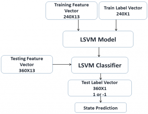
The block diagram of the proposed system is shown in Figure 1.
3.1 Preprocessing
Preprocessing is a very important step to prepare the dataset, minimize the noise, and to enhance the image features. The following subsections will discuss that deeply.
Getting the frames and do the Enhancement
As discussed before there are five subjects and the dataset was constructed to be 600 frames (60 frame [randomly selected] Χ 2 [states] Χ 5 [participants]). The train partition contains randomly selected forty percent of data (240 frames) and the remaining 360 frames construct the testing part. The target is to extract each frame from the given test set to be in "Alert" or "Fatigue" state.
Figure 1. Block diagram of the proposed system
As filtration is a crucial step in eliminating noise; "Homomorphic" and "Median" filters are applied.
The image is first converted to grayscale (as working on gray image will reduce the processing time), and then a homomorphic filter is applied to it. The homomorphic filter involves applying a fast fourier transform to the image and then passing it through a high pass filter. For this, Butterworth's high pass filter was used. The homomorphic filter reduces inconsistency in the background illumination [22], making image segmentation easier. The image is then passed through a median filter to remove any salt and pepper noise [23].
Detecting the face and cropping the eyes and mouth
As discussed before there are five subjects and the dataset was constructed to be 600 frames (60 frame [randomly selected] Χ 2 [states] Χ 5 [participants]). The train partition contains randomly selected forty percent of data (240 frames) and the remaining 360 frames construct the testing part. The target is to extract each frame from the given test set to be in "Alert" or "Fatigue" state.
Viola-Jones Algorithm [24]
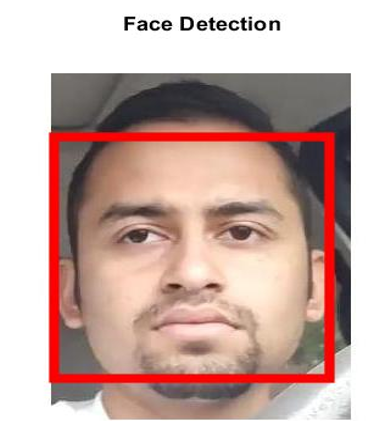
A key component of face recognition is face detection. Any system that identifies people must be able to detect faces in images. Face recognition algorithms can be developed quickly with Viola-Jones Object Detection Frame. By analyzing the pixels within full frontal photographs, real-time detection can be achieved. In addition to poses and objects that obscure the face or tilt the head, there are other factors that need to be considered or addressed. This algorithm's primary purpose is to correctly detect faces in images [25].
There are several advantages to the Viola-Jones algorithm:
Figure 2. Example of face detection
In this work, MATLAB computer vision toolbox was used to detect face, mouth and eyes based on "Viloa-Jones" technique.
When applied on participant number (4); Figures 2, 3 and 4 show examples of the results of detecting face, eyes, and mouth respectively.
Figure 3. Example of eyes detection
Figure 4. Example of mouth detection
3.2 Constructing features vector
This step is constructed from the succession of the calculations of the frames of all five subjects (120 frames = 60 frames for each subject * two inspected states). As previously mentioned, the train set of the subject consists of 240 images (40% of 600) and the test set of the subject consists of the remaining 360 images.
3.3 Classification
For traditional classifiers [1st approach] [26-28]
Diagonal Linear Discriminant Analysis
A linear classifier uses linear functions to determine how different groups are classified. It is widely acknowledged that these classifiers are the most well-known BCI algorithms.
Data representing different classes are separated using hyper-planes in LDA [29, 30]. In a two-class problem, the class of a function vector is determined by its position in the hyper-plane.
The diagonal covariance matrices for both groups are equal in diagonal linear discriminant analysis, which assumes that the data has a normal distribution. The separating hyper-plane is found by looking for the projection that minimizes interclass variance by maximizing the distance between the means of two classes [30].
DiagLDA
As shown in Figure 5, in the first approach, the "DiagLDA method," a test label of '1' was specified as target (Fatigue) or '-1' as non-target (Normal) throughout each trial.
Figure 5. DiagLDA classifier
Support Vector Machine (SVM)
This classifier is used to classify a set of binary labeled data; it also employs a hyper-plane to divide the data into two groups [31, 32]. Then, after training the classifier on a specific dataset, the hyper-plane is optimized and chosen based on the maximum gap between the hyper-plane and that data. This is accomplished by transferring data from the input area to the feature area, where linear classification is realized.
Linear support vector machine classification allows for classification with linear decision boundaries. These classifiers have been used successfully to solve a large number of concurrent BCI problems [33-36].
Figure 6. SVM classifier
SVMs have a number of advantages. SVMs are thought to have strong generalization properties [32, 37], to be resistant to overtraining [37], and to be immune to the curse of dimensionality [31, 32].
SVMs have been used in brain research because they are a strong pattern recognition approach, especially when dealing with high-dimensional problems [36]. The proposed algorithm is depicted in Figure 6.
In the set of train data used earlier as a validation set, Table 2 shows the values of the regularization parameters (hyper-parameters) chosen through cross-validation.
Table 2. Values of SVM hyper-parameters
|
Kernel Function |
Kernel Scale |
Standardize |
|
Linear |
25.4 |
True |
K-Nearest Neighbors (KNN)
The K-nearest neighbor (KNN) method of supervised classification learning is used to classify samples. The goal of this algorithm is to identify a new sample by using its features and previously labeled training samples [38]. The algorithm is memory-based and does not require model fitting. The closest k training points (Euclidean distance) to a query point x0 are found. The new query is assigned to a cluster based on the number of neighbors it has. Any voting bonds that are broken will be broken at random [39].
As shown in Figure 7, the KNN (with N=5) method is used as a classifier in this work that can be used in brain research.
Figure 7. KNN classifier
Random Forest Classifier (RFC)
Random forests are machine learning schemes derived from decision trees, where a decision tree is a tree-like diagram used to determine a course of action. Every branch of the tree represents a possible option, event, or reaction [40].
Some of the advantages of using Random Forests are as follows:
1. No over fitting: Using multiple trees reduces the likelihood of over fitting as well as the time required to practice.
2. High precision: it performs well in large databases and makes highly accurate predictions for large datasets. This is critical in today's big data world, and it's likely where Random Forest shines.
3. Estimate missing data: When a large portion of the data is missing, Random Forest guesses which one is best suited for the missing parameter.
In this paper, a Random Forest classifier (number of trees=10) algorithm is used.
3.4 State prediction
The previously discussed classifiers nearly specify the state. The following section will present an analysis of the work from various perspectives.
For deep learning [2nd approach]
The basis of today's deep learning algorithms is the computer simulation of a neuron in the human brain.
It is a process that has emerged by trying to do it. Neural networks of Donald Hebb's nerve cell and it started with an examination of its structure. Then, mathematically modeling the model in the computer environment.
The creation of artificial neural networks is known as the starting point [41] of the artificial nerve.
In the emergence and progress of networks, years have passed and the term deep learning has been used in recent years and the studies have focused on this issue.
Deep learning is especially used for classification, recognition and detection [42] and the studies have gained weight in this direction. Recently, deep learning algorithms have been used in many technological structures in our daily life.
Achieving high performances has increased the tendency to this issue. Many classifications made recognition studies are available.
In deep learning architectures, there are several different learning strategies during the training of the network.
These are teacher learning, teacher-less learning, and reinforcement learning.
In teacher learning; the information of what the input data at the input of the network is at the output is given. The weights of the network are the same.
It is repeatedly inserted into the network as input data so that the weights of the network are adjusted accordingly.
Thus, the weights are determined by training the network [43].
In teacher-less learning; no information is given about what the input data is at the output. Every data that enters the network has a data belonging to a nearby cluster at the exit takes value. Thus, each data becomes a member of a cluster at the output [44, 45].
In reinforcement learning, on the other hand, the information of what the input data is at the output is not given in the network. Exit information is given as to whether it is true or false. It is assigned a value of 1 if true and 0 if false. According to this the training of the network is performed [46].
The deep learning structure represents an advanced structure of the convolutional neural network. With the convolution process, the features of the input data are automatically extracted and added to the next layers sent with these attributes.
The convolution process extracts distinctive features from an image.
In the convolutional neural network, a separate process is carried out in each layer and data is transferred to the next layer. Each layer performs its own function. Layers in deep learning architectures and the operations performed by these layers are as follows:
It is formed by traversing a matrix of size. The specified small size matrices are the whole image.
It hovers over the matrix, highlighting the features in the image and a new image matrix is obtained [47].
It is a 16 convolutional 3 fully connected layer network created after the algorithm. Maxpool, a total of 47 layers with Fullconnectedlayer, Relulayer, Dropoutlayer and Softmaxlayer layers.
VggNet has a different structure from traditional sequential network architecture such as AlexNet.
Because the used network is a large network (50 sections); Figure 8 shows just the first section.
Figure 8. First section of used "ResNet-50" model
Table 3 shows some values of the parameters chosen through training and testing of the data using the previously mentioned model.
Table 3. Values of some parameters used with "ResNet-50" model
|
Parameter |
Selected Value |
|
featureLayer |
fc1000 |
|
MiniBatchSize |
32 |
|
Learning |
Linear |
|
LossFunction |
'crossentropyex' |
|
Learning Rate |
0.01 |
Results of applying the suggested classification techniques will be presented and discussed in the following section.
4.1 For traditional classifiers [1st approach]
First: Looking at all five subject together
The accuracy of the estimated trials in the test sets is determined by the percentage of those that are correctly estimated. Based on the features extracted from images of both eyes and mouth, the accuracies concerning all subjects and the results for each classifier are shown in Table 4. As shown in Table 5; the time taken to train the classifier and predict a trial state does not exceed 4 seconds. The resulted times are reliable and make the system suitable for real-time applications.
Figure 9 shows the accuracies calculated when applying the discussed classifiers for the dataset taken from all five subjects together.
By comparing the accuracies of the proposed classifiers, it is clearly shown that random forest (RF) and KNN algorithms give the highest accuracies, as they performed 91.94%. However, the DiagLDA method gave the lowest results as it achieved accuracy of 68.89%.
Table 4. "All subjects" [Eyes+Mouth] acc. of classifiers
|
Classifiers |
The Whole Subjects 5 Subjects as a unit |
|
|
Features Used (13) |
Accuracy |
|
|
DiagLDA |
Contrast Energy Standard Deviation Homogeneity Mean Correlation Entropy Kurtosis Variance Smoothness RMS IDM Skewness |
68.89% |
|
SVM Linear |
90.28% |
|
|
KNN N=5 |
91.94% |
|
|
RF T=10 |
91.94% |
|
Table 5. "All subjects" [Eyes+Mouth] time taken for the applied classifiers
|
Classifiers |
Whole Subjects |
|
|
Train Time (sec.) / Trial |
Test Time (sec.) / Trial |
|
|
DiagLDA |
0.351463 |
1.238408 |
|
SVM Linear |
0.237492 |
0.715007 |
|
KNN N=5 |
0.551861 |
0.649169 |
|
RF T=10 |
1.352904 |
1.861519 |
Figure 9. Accuracies of the applied classifiers
Table 6. "All subjects" [Eyes-Only] acc. of classifiers
|
Classifiers |
The Whole Subjects 5 Subjects as a unit |
|
|
Features Used (13) |
Accuracy |
|
|
DiagLDA |
Contrast Energy Standard Deviation Homogeneity Mean Correlation Entropy Kurtosis Variance Smoothness RMS IDM Skewness |
68.89% |
|
SVM Linear |
78.89.28% |
|
|
KNN N=5 |
81.39% |
|
|
RF T=10 |
81.39% |
|
For the eyes features only, the accuracies concerning all subjects and the results for each classifier are shown in Table 6. Whereas, Figure 10 shows the accuracies calculated when applying the discussed classifiers for the dataset taken from all five subjects together.
Figure 10. Accuracies of the applied classifiers
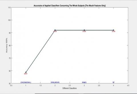
Table 7 and Figure 11 show the accuracies concerning all subjects and the results for each classifier when dealing with the mouth features only.
Table 7. "All subjects" [Mouth-Only] acc. of classifiers
|
Classifiers |
The Whole Subjects 5 Subjects as a unit |
|
|
13 Features Used |
Accuracy |
|
|
DiagLDA |
Contrast Energy Standard Deviation Homogeneity Mean Correlation Entropy Kurtosis Variance Smoothness RMS IDM Skewness |
58.61% |
|
SVM Linear |
91.94% |
|
|
KNN N=5 |
91.94% |
|
|
RF T=10 |
91.94% |
|
Second: Looking at each subject individually
Now every subject is taken separately and the building of training and testing data is based on the same criteria (40% as Training and the remaining 60% as Testing).
Based on the features extracted from images of both eyes and mouth, the accuracies concerning each subject and the results for each classifier are shown in Table 8.
Figures 12 and 13 show the accuracies calculated when applying the discussed classifiers for the dataset taken from each five subjects together.
By comparing the accuracies of the proposed classifiers, it is clearly shown that subjects (1), (3), and (5) gave the highest performance for all classifiers, as they accomplished 100%. However, subject (2) gave the lowest results for all classifiers except random forest (RF) as it achieved maximum accuracy of 45.83% for the remaining 3 classifiers.
Figure 11. Accuracies of the applied classifiers
Table 8. "Subjects 1 - 5" accuracies of the applied classifiers
|
Classifiers |
Accuracy |
||||
|
Subject 1 |
Subject 2 |
Subject 3 |
Subject 4 |
Subject 5 |
|
|
DiagLDA |
100% |
45.83% |
100% |
52.78% |
100% |
|
LSVM |
100% |
45.83% |
100% |
47.22% |
100% |
|
KNN N=5 |
100% |
45.83% |
100% |
52.78% |
100% |
|
RF T=10 |
100% |
54.17% |
100% |
52.78% |
100% |
Therefore, four classifiers' performances and evaluation measurements will be computed: accuracy, sensitivity, specificity, and precision.
From previously presented work, the full details concerning the classifiers' performances and the confusion matrices dealing with the features extracted from images of both eyes and mouth will be shown in the following part.
Positive observations mean that the observer is observing the target (Fatigue/Drowsy) and negative means that the observer is not observing the target (Normal/Alert):
- "True positives" (T.P.) are observations that are both positive and predictable.
- "False positives" (F.P.): occur when an observation is negative, however the prediction is positive.
- "True negatives" (T.N.): are observations that are both negative and predictable.
- "False negatives" (F.N.): occur when an observation is positive, however the prediction is negative.
Table 9. Confusion matrices for all classifiers on the data
|
DiagLDA |
Actual Value |
||
|
(Target) Positive |
(Non-Target) Negative |
||
|
Predicted Value |
(Target) Positive |
T.P.=113 |
F.P.=41 |
|
(Non-Target) Negative |
F.N.=71 |
T.N.=135 |
|
|
LSVM |
Actual Value |
||
|
(Target) Positive |
(Non-Target) Negative |
||
|
Predicted Value |
(Target) Positive |
T.P. = 149 |
F.P. = 0 |
|
(Non-Target) Negative |
F.N. = 35 |
T.N. = 176 |
|
|
KNN(N=5) |
Actual Value |
||
|
(Target) Positive |
(Non-Target) Negative |
||
|
Predicted Value |
(Target) Positive |
T.P.=184 |
F.P.=29 |
|
(Non-Target) Negative |
F.N.=0 |
T.N.=147 |
|
|
Random Forest(T =10) |
Actual Value |
||
|
(Target) Positive |
(Non-Target) Negative |
||
|
Predicted Value |
(Target) Positive |
T.P.=149 |
F.P.=0 |
|
(Non-Target) Negative |
F.N.=35 |
T.N.=176 |
|
Figure 12. Accuracies of the applied classifiers on Subjects 1 – 5
Figure 13. Accuracies of the applied classifiers on all subjects individually
Figure 14. ROC Curves of the applied classifiers
The actual and predicted testing data are 360 observations (600 observations [Normal and Fatigue] Χ 60% The testing part).
As shown in Table 9, all classes' confusion matrices are shown for the four classifiers.
Table 10 shows the accuracies calculations for the five classifiers performed on all participants' (subjects') data using all features.
The Receiver Operating Characteristic (ROC) curve is a common visual representation of a classification model's output. It summarizes the trade-off between the true positive rate (TPR) and the false positive rate (FPR) for various likelihood thresholds in a predictive model. ROC curves for the four tried classifiers concerning all subjects are shown in Figure 14.
Table 10. Performances calculations for all applied classifiers
|
Classifiers |
From electrodes (F4, FCZ, and O2) for all subjects |
|||
|
Accuracy |
Precision |
Sensitivity |
Specificity |
|
|
DiagLDA |
68. 8889% |
73.3766% |
61.4131% |
66.8639% |
|
SVM (Linear) |
90.2778% |
100% |
80.9783% |
89.4895% |
|
KNN (N=5) |
92.6952% |
86.3849% |
100% |
92.6952% |
|
Random Forest (T=10) |
90.2778% |
100% |
80.9783% |
89.4895% |
Results in Tables 9 and 10 show that all the suggested classifiers achieve high performance, except for the "DiagLDA" classifier. According to the ROC curves analysis shown in Figure 14, the areas under the curves (AUC) of the applied classifiers (SVM[Linear], KNN[N=5], and RF[T=10]) yield relatively high results (more than 0.90). Therefore, the classifiers presented here are appropriate models.
4.2 For deep learning model [2nd approach]
In this section, the analysis and evaluation of the suggested deep neural network model has been carried out.
Table 11 and Figure 15 depict the confusion matrix for the presented model.
Table 11. Confusion matrices for applied CNN model regarding the image data from all subjects
|
Deep Learning Resnet-50 |
Actual Value |
||
|
(Target) Positive |
(Non-Target) Negative |
||
|
Predicted Value |
(Target) Positive |
T.P.=155 |
F.P.=0 |
|
(Non-Target) Negative |
F.N. = 13 |
T.N. = 192 |
|
Figure 15. Plotting confusion matrices for applied CNN model regarding the image data from all subjects
The performances calculations of the tried CNN model performed on all participants' (subjects') are shown in Table 12.
The Receiver Operating Characteristic (ROC) Curve is a common visual representation of a classification model's output. It summarizes the trade-off between the true positive rate (TPR) and the false positive rate (FPR) for various likelihood thresholds in a predictive model. ROC curve for the presented model is shown in Figure 16.
Table 12. Performances calculations for "Resnet-50" classifier
|
Classifier |
From electrodes (F4, FCZ, and O2) for all subjects |
|||
|
Accuracy |
Precision |
Sensitivity |
Specificity |
|
|
"Resnet-50" Deep Learning Model |
96. 3889% |
100% |
92.2619% |
95.9752% |
Figure 16. ROC curves for applied CNN model
4.3 Comparative analysis
Several research groups have used driver face images to study driver fatigue detection in recent years to resolve this issue. Table 12 describes the related classification methods used in some studies. This indicates that the results obtained by applying the proposed classification methods were better than that presented below in Table 13 despite of utilizing fewer features extracted from eyes and mouth driver images.
Table 13. Accuracies from various researchers
|
# |
Research Group |
Acc. |
Center of Research |
Technique |
|
1 |
Fabian Friedrichs |
82.5% |
The Department of System Theory and Signal Processing at Stuttgart University, Germany |
Using a camera-based drowsiness measurement for driver state |
|
2 |
Wei Zhang |
86% |
Tsinghua University, Department of Automotive Engineering, Beijing 100084, China, State Key Laboratory of Automotive Safety and Energy |
A total of six measures are calculated based on percentage of eyelid closure, maximum closure duration, the blink frequency, the number of times the eyes open, and the speed at which they close. |
|
3 |
Ralph Oyini Mbouna |
91.1% |
University of Chungbuk, Cheongju 361-763, Korea, Department of Electronics Engineering |
This system uses visual features such as the eye index (EI), pupil activity (PA), and head pose (HP) in order to determine a driver's level of alertness |
|
4 |
Eyosiyas Tadesse |
93.5% |
Chinese Convention and Exhibition Center, Hong Kong |
To detect drowsiness, they developed a method based on Hidden Markov Models (HMMs) to examine the driver's facial expressions |
|
5 |
Gustavo A |
87% |
Research Laboratory for Intelligent Systems, Department of Systems Engineering & Automation, University Carlos III of Madrid, 28911 Leganés, Spain |
With the help of two-dimensional and three-dimensional algorithms, the system provides head pose estimation and identification of regions of interest |
|
6 |
This work |
96.4% |
Misr University for Science and Technology, Faculty of Engineering, Giza, Egypt |
Using "Resnet-50" deep learning model as a classifier |
In traffic safety, detecting driver exhaustion has a clear application for warning of driving fatigue, minimizing unnecessary driving accidents. Future research should concentrate on two areas:
1- Integrating EEG signals with face images acquired from driver to make a hybrid system.
2- Making our own dataset and validate it.
The time variability of fatigue data can aid in determining the degree of uncertainty in a system's data variables and capturing the sensitivity of the obtained results [48, 49]. EEG datasets from another online experiment in this study were subjected to an offline review. Since the offline and online classifications have different features, a follow-up analysis in a real-time online experimental setting is required to validate the results of this study [26].
An objective system for detecting drowsy driving in a driver face image-based framework was suggested in this study. Four classifiers were utilized for training and testing data, data was preprocessed before extracting feature, and also a deep convolutional neural network model was utilized for comparison purpose and to demonstrate the efficacy and robustness of the proposed method. Since it reported high performance especially with the deep learning model, the results suggested that this type of technology could be useful for detecting drowsy driving.
It is predicted that an image-based system for drowsiness observation in appropriate areas, or a competitive function with presented methods, would be feasible. Although, there are many problems in the future that will need to be addressed. The study needs to be replicated with a large group of people and real-time driving images. The reliability and comfort of different techniques using other features for real-time monitoring of driver drowsiness should be the subject of future studies.
The dataset analyzed during the current study is available from University of Texas at Arlington, "Computer Science and Engineering Department" website. This dataset was derived from the following public domain resource:
http://vlm1.uta.edu/~athitsos/projects/drowsiness/?C=D;O=A [Last modified Sep-2020].
[1] Puvanachandra, P., Hoe, C., El-Sayed, H.F., Saad, R., Al-Gasseer, N., Bakr, M., Hyder, A.A. (2012). Road traffic injuries and data systems in Egypt: Addressing the challenges. Traffic Injury Prevention, 13(sup1): 44-56. https://doi.org/10.1080/15389588.2011.639417
[2] Poursadeghiyan, M., Mazloumi, A., Saraji, G.N., Baneshi, M.M., Khammar, A., Ebrahimi, M.H. (2018). Using image processing in the proposed drowsiness detection system design. Iranian Journal of Public Health, 47(9): 1371-1378.
[3] Poursadeghiyan, M., Mazloumi, A., Saraji, G.N., Niknezhad, A., Akbarzadeh, A., Ebrahimi, M.H. (2017). Determination the levels of subjective and observer rating of drowsiness and their associations with facial dynamic changes. Iranian Journal of Public Health, 46(1): 93-102.
[4] Vesselenyi, T., Moca, S., Rus, A., Mitran, T., Tătaru, B. (2017). Driver drowsiness detection using ANN image processing. In IOP Conference Series: Materials Science and Engineering, 252(1): 012097. https://doi.org/10.1088/1757-899X/252/1/012097
[5] Kholerdi, H.A., TaheriNejad, N., Ghaderi, R., Baleghi, Y. (2016). Driver's drowsiness detection using an enhanced image processing technique inspired by the human visual system. Connection Science, 28(1): 27-46. https://doi.org/10.1080/09540091.2015.1130019
[6] Li, M.A., Zhang, C., Yang, J.F. (2010). An EEG-based method for detecting drowsy driving state. In 2010 Seventh International Conference on Fuzzy Systems and Knowledge Discovery, 5: 2164-2167. https://doi.org/10.1109/FSKD.2010.5569757
[7] Correa, A.G., Leber, E.L. (2010). An automatic detector of drowsiness based on spectral analysis and wavelet decomposition of EEG records. In 2010 Annual International Conference of the IEEE Engineering in Medicine and Biology, pp. 1405-1408. https://doi.org/10.1109/IEMBS.2010.5626721
[8] Vicente, J., Laguna, P., Bartra, A., Bailón, R. (2011). Detection of driver's drowsiness by means of HRV analysis. In 2011 Computing in Cardiology, 89-92.
[9] Suryaprasad, J., Sandesh, D., Saraswathi, V., Swathi, D., Manjunath, S. (2013). Real time drowsy driver detection using haarcascade samples. In CS & IT Conference Proceedings, 3(8): 45-54.
[10] Ingre, M., Åkerstedt, T., Peters, B., Anund, A., Kecklund, G. (2006). Subjective sleepiness, simulated driving performance and blink duration: examining individual differences. Journal of Sleep Research, 15(1): 47-53. https://doi.org/10.1111/j.1365-2869.2006.00504.x
[11] Bergasa, L.M., Nuevo, J., Sotelo, M.A., Barea, R., Lopez, M.E. (2006). Real-time system for monitoring driver vigilance. IEEE Transactions on Intelligent Transportation Systems, 7(1): 63-77. https://doi.org/10.1109/TITS.2006.869598
[12] Fischer, J., Seitz, D., Verl, A.W. (2010). Face detection using 3-D time-of-flight and colour cameras. ISR/ROBOTIK 2010, Proceedings for the joint conference of ISR 2010 (41st Internationel Symposium on Robotics) und ROBOTIK 2010 (6th German Conference on Robotics), 7-9 June 2010, Munich, Germany.
[13] Adi, K., Widodo, A.P., Widodo, C.E., Putranto, A.B., Naqiyah, S., Aristia, H.N. (2019). Detecting driver drowsiness using total pixel algorithm. In Journal of Physics: Conference Series, 1217(1): 012036. https://doi.org/10.1088/1742-6596/1217/1/012036
[14] Adi, K., Widodo, C.E., Widodo, A.P., Gernowo, R., Pamungkas, A., Syifa, R.A. (2018). Detection lung cancer using gray level co-occurrence matrix (GLCM) and back propagation neural network classification. Journal of Engineering Science & Technology Review, 11(2): 8-12. https://doi.org/10.25103/jestr.112.02
[15] Gonzalez, R.C., Woods, R.E., Eddins, S.L. (2009). Digital Image Processing Using MATLAB. 2nd ed. Gatesmark Publishing, United Stated of America, 12-67.
[16] Adi, K., Suksmono, A.B., Mengko, T.L.R., Gunawan, H. (2010). Phase unwrapping by Markov chain Monte Carlo energy minimization. IEEE Geoscience and Remote Sensing Letters, 7(4): 704-707. https://doi.org/10.1109/LGRS.2010.2046393
[17] Jain, A.K. (1986). Fundamental of Digital Image Processing. Prentice Hall, United State of America, 49-75.
[18] Wilhelm, B., Mark, J.B. (2007). Digital Image Processing: An Algorithmic Approach Using Java. Springer-Verlag, New York, 199-234.
[19] Revathy, N., Guhan, T. (2012). Face recognition system using back propagation artificial neural networks. International Journal of Computer Science and Information Technology, 11: 68-77.
[20] Ghoddoosian, R., Galib, M., Athitsos, V. (2019). A realistic dataset and baseline temporal model for early drowsiness detection. 2019 IEEE/CVF Conference on Computer Vision and Pattern Recognition Workshops (CVPRW), pp. 178-187. https://doi.org/10.1109/CVPRW.2019.00027
[21] Athitsos, V. (2020). Drowsiness Detection Project Dataset. http://vlm1.uta.edu/~athitsos/projects/drowsiness/?C=D;O=A, accessed on 11 November 2021.
[22] Hill, P.R., Bhaskar, H., Al-Mualla, M.E., Bull, D.R. (2016). Improved illumination invariant homomorphic filtering using the dual tree complex wavelet transform. In 2016 IEEE International Conference on Acoustics, Speech and Signal Processing (ICASSP), pp. 1214-1218. https://doi.org/10.1109/ICASSP.2016.7471869
[23] Gonzalez, R.C., Woods, R.E. (2002). Digital Image Processing. Pearson Education.
[24] Viola, P., Jones, M. (2001). Rapid object detection using a boosted cascade of simple features. In Proceedings of the 2001 IEEE Computer Society Conference on Computer Vision and Pattern Recognition, CVPR 2001, 1: I-I. https://doi.org/10.1109/CVPR.2001.990517
[25] Viola, P., Jones, M.J. (2004). Robust real-time face detection. International Journal of Computer Vision, 57(2): 137-154. https://doi.org/10.1023/B:VISI.0000013087.49260.fb
[26] Fouad, I.A., Labib, F.E.Z.M., Mabrouk, M.S., Sharawy, A.A., Sayed, A.Y. (2020). Improving the performance of P300 BCI system using different methods. Network Modeling Analysis in Health Informatics and Bioinformatics, 9(1): 1-13. https://doi.org/10.1007/s13721-020-00268-1
[27] Fouad, I.A. (2021). A robust and reliable online P300-based BCI system using Emotiv EPOC+ headset. Journal of Medical Engineering & Technology, 45(2): 94-114. https://doi.org/10.1080/03091902.2020.1853840
[28] Labib, F.E.Z.M., Fouad, I.A., Mabrouk, M.S., Sharawy, A.A. (2020). Multiple classification techniques toward a robust and reliable P300 BCI system. Biomedical Engineering: Applications, Basis and Communications, 32(2): 2050010. https://doi.org/10.4015/S1016237220500106
[29] Stork, D.G., Duda, R.O., Hart, P.E., Stork, D. (2001). Pattern Classification. A Wiley-Interscience Publication.
[30] Fukunaga, K. (1990). Statistical Pattern Recognition. second edition, ACADEMICPRESS, INC.
[31] Burges, C.J. (1998). A tutorial on support vector machines for pattern recognition. Data Mining and Knowledge Discovery, 2(2): 121-167. https://doi.org/10.1023/A:1009715923555
[32] Bennett, K.P., Campbell, C. (2000). Support Vector Machines: Type Explorations Newslette, 2:1.
[33] Blankertz, B., Kawanabe, M., Tomioka, R., Hohlefeld, F., Müller, K.R., Nikulin, V. (2007). Invariant common spatial patterns: Alleviating nonstationarities in brain-computer interfacing. Advances in Neural Information Processing Systems, 20.
[34] Garrett, D., Peterson, D.A., Anderson, C.W., Thaut, M.H. (2003). Comparison of linear, nonlinear, and feature selection methods for EEG signal classification. IEEE Transactions on Neural Systems and Rehabilitation Engineering, 11(2): 141-144. https://doi.org/10.1109/TNSRE.2003.814441
[35] Rakotomamonjy, A., Guigue, V., Mallet, G., Alvarado, V. (2005). Ensemble of SVMs for improving brain computer interface P300 speller performances. In International Conference on Artificial Neural Networks, pp. 45-50. https://doi.org/10.1007/11550822_8
[36] Rakotomamonjy, A., Guigue, V. (2008). BCI competition III: Dataset II-ensemble of SVMs for BCI P300 speller. IEEE Transactions on Biomedical Engineering, 55(3): 1147-1154. https://doi.org/10.1109/TBME.2008.915728
[37] Jain, A.K., Duin, R.P.W., Mao, J. (2000). Statistical pattern recognition: A review. IEEE Transactions on Pattern Analysis and Machine Intelligence, 22(1): 4-37. https://doi.org/10.1109/34.824819
[38] Hastie, T., Tibshirani, R., Friedman, J.H., Friedman, J.H. (2009). The Elements of Statistical Learning: Data Mining, Inference, and Prediction. Springer, New York, NY. https://doi.org/10.1007/978-0-387-21606-5
[39] Schütze, H., Manning, C.D., Raghavan, P. (2008). Introduction to Information Retrieval. Cambridge: Cambridge University Press.
[40] Olson, M. (2018). Essays on random forest ensembles. Ph.D. Thesis. 3420 Walnut St., Philadelphia, PA 19104‐6206.
[41] Hebb, D.O. (2005). The Organization of Behavior: A Neuropsychological Theory. Psychology Press. https://doi.org/10.4324/9781410612403
[42] Deng, L., Yu, D. (2014). Deep learning: methods and applications. Foundations and Trends in Signal Processing, 7(3–4): 197-387. https://doi.org/10.1561/2000000039
[43] Makantasis, K., Karantzalos, K., Doulamis, A., Doulamis, N. (2015). Deep supervised learning for hyperspectral data classification through convolutional neural networks. In 2015 IEEE International Geoscience and Remote Sensing Symposium (IGARSS), pp. 4959-4962. https://doi.org/10.1109/IGARSS.2015.7326945
[44] Radford, A., Metz, L., Chintala, S. (2015). Unsupervised representation learning with deep convolutional generative adversarial networks. arXiv preprint arXiv:1511.06434. https://doi.org/10.48550/arXiv.1511.06434
[45] Higgins, I., Matthey, L., Glorot, X., Pal, A., Uria, B., Blundell, C., Lerchner, A. (2016). Early visual concept learning with unsupervised deep learning. arXiv preprint arXiv:1606.05579. https://doi.org/10.48550/arXiv.1606.05579
[46] Papernot, N., Abadi, M., Erlingsson, U., Goodfellow, I., Talwar, K. (2016). Semi-supervised knowledge transfer for deep learning from private training data. arXiv preprint arXiv:1610.05755. https://doi.org/10.48550/arXiv.1610.05755
[47] Liu, L., Shen, C., Van den Hengel, A. (2015). The treasure beneath convolutional layers: Cross-convolutional-layer pooling for image classification. In Proceedings of the IEEE Conference on Computer Vision and Pattern Recognition, pp. 4749-4757.
[48] Convertino, M., Muñoz-Carpena, R., Kiker, G.A., Perz, S.G. (2015). Design of optimal ecosystem monitoring networks: hotspot detection and biodiversity patterns. Stochastic Environmental Research and Risk Assessment, 29(4): 1085-1101. https://doi.org/10.1007/s00477-014-0999-8
[49] Lüdtke, N., Panzeri, S., Brown, M., Broomhead, D.S., Knowles, J., Montemurro, M.A., Kell, D.B. (2008). Information-theoretic sensitivity analysis: A general method for credit assignment in complex networks. Journal of The Royal Society Interface, 5(19): 223-235. https://doi.org/10.1098/rsif.2007.1079