Lu Feng | Peng Wu* | Linhua Zheng
© 2022 IIETA. This article is published by IIETA and is licensed under the CC BY 4.0 license (http://creativecommons.org/licenses/by/4.0/).
OPEN ACCESS
Roll rate estimation is essential to attitude measurement. During the processing of baseband signals, it is complicated to measure the vehicle rolling attitude, based on the energy features of existing satellite signals. To measure the energy of received signals in real time, the data communication interface and storage unit of the receiving device must be customized. However, the customization will push up the cost of attitude sensors, and result in processing delays. To solve the problem, this paper measures the vehicle roll rate by the variation features of pseudorange observations, which are easy to acquire and highly applicable. Specifically, the roll rate of a cylindrical spinning vehicle was estimated, using Global Navigation Satellite System (GNSS) receiver with single side-mounted antenna. After analyzing the variation of pseudorange observations, the authors calculated the roll rate of the cylindrical spinning vehicle based on the variation rules. The proposed approach was verified through experiments with simulated GNSS signals. The accuracy of our approach was measured at different rotation speeds and translational speeds. The results show that our approach can accurately estimate the roll rate when the standard deviations of noise is less than 1m for pseudorange measurement.
Global Navigation Satellite System (GNSS), spinning vehicle, baseband signal processing, pseudorange observations, roll rate estimation
The flight trajectory estimation and flight process control of high-speed vehicles or other projectiles hinge on the acquisition of the attitude information. Inaccurate attitude information will undermine the precision of the control system, and even destabilize the vehicles. Several kinds of sensors are available to obtain the attitude information of an aircraft, including inertial navigation system (INS), geomagnetic sensor, gyroscope, and satellite navigation receiver, to name but a few. All these sensors can provide accurate attitude information, facilitating the subsequent control of the aircraft. For a cylindrical vehicle, rotation should be accompanied by translational motions to ensure flight stability. But the rotation state may influence the measurement of vehicle attitude [1-3].
In attitude measurement, initial alignment is a necessary step for inertial devices. If the vehicle spins, the fast rotation will disturb the normal operation of many inertial devices. Even a slight gyroscopic error in the integration process will lead to a large and rapid change of attitude error. What is worse, the inertial devices may fail in the launch stage, due to the high overload of the vehicle [4, 5].
The geomagnetic sensor clearly displays the phase relationship of speed waveforms, supports the measurements in a wide range of speeds, and captures speed variations clearly and stably. However, the geomagnetic sensor is susceptible to changes in motor and external magnetic field, as well as the magnetic shielding effect of the vehicle or emitter. The magnetic field signals would be underestimated, especially when the sensitive axis of the local magnetic sensor is parallel to the geomagnetic line. This limits the application of the geomagnetic sensor in spinning vehicles [6]. In addition, the geomagnetic sensor may complicate the mechanical structure of the satellite navigation receiver, given the high cost of the sensor, and the complexity of the attitude measurement algorithm.
In the early 20th century, some scholars proposed to measure rolling attitude with the Global Positioning System (GPS) [7]. With a simple structure, the Global Navigation Satellite System (GNSS) receiver can simultaneously acquire the position and rolling attitude at a low cost. Based on the GNSS receiver, the roll attitude can be measured by two modes: the multi-antenna mode, and the single-antenna mode [8-11].
In the multi-antenna mode, multiple antennas are usually mounted on the surface of the same cross-section of a cylindrical spinning vehicle, so that at least one antenna can receive satellite signals at any time [12]. Doty et al. determined the rolling attitude of cylindrical spinning vehicles based on the amplitude correlation of GNSS signals received by multiple antennas [13-15]. The roll rate was taken as prior information to ensure the accuracy of attitude estimation, and the signals received by multiple antennas were combined into one signal. However, the combined signal is prone to mutual interference, and highly noisy, compared with each single signal. There are several drawbacks of multi-antenna attitude measurement: the complexity of system and computation, the high cost, and the poor real-time performance [16, 17].
In the single-antenna mode, the antenna is usually deployed on the side of the aircraft, which rotates with the cylindrical spinning vehicle on its cross-section around the spinning axis. The spinning of the vehicle has a modulation effect on the GNSS signal received by the single antenna [18]. Shen et al. presented an algorithm, which regards the rotation-induced Doppler frequency shift with sine variation as the noise of a fixed frequency, in the absence of roll rate as prior information. The rotation-induced Doppler frequency shift was eliminated by the filter in the vehicle tracking loop [19-21]. Kim et al. proposed a design method for the GNSS receiver tracking loop of spinning vehicles. In their method, the influence of rotation on the GNSS signal was eliminated by adding a rotation tracking loop into the conventional receiver [22, 23]. The additional loop tracked the rotation angle and frequency of the vehicles.
Admittedly, the methods above can solve the signal interference between multiple antenna measurements, and simplify the mechanical structure of the system. Nevertheless, the commonly used GNSS receiver does not directly output the amplitude of the received GNSS signals, which is needed by the above methods for estimating the rotation frequency. The receiver must be customized to output the signal amplitude in real time, which is bound to push up the cost. Therefore, the existing methods only work well in the presence of expensive customized receivers, and perform poorly in non-customized scenarios [24]. None of the existing studies has estimated attitude using the GNSS observations by the conventional receiving function.
Through the preliminary studies, it can be concluded that: the real-time pseudorange measured by the GNSS receiver will oscillate periodically with the rotation of the cylindrical spinning vehicle, if the phase center of the single antenna in the GNSS receiver does not coincide with the centroid of the cylindrical spinning vehicle, and if the single antenna rotates around the cross-section of the cylindrical spinning vehicle. Therefore, this paper tries to estimate the roll speed of the cylindrical spinning vehicle based on real-time observations of pseudorange, aiming to reasonably customize the energy of output signals, and solve the common problems of the existing algorithms (e.g., numerous loop filtering / integral operations). Specifically, the pseudorange variation frequency caused by the rotation of the vehicle was extracted through a frequency analysis of pseudorange observations. The pseudorange spectrum was smoothed, according to the angle between the rotation plane of the receiver and the line of sight (LOS) vector. Our approach involves only a few differential operations, and fast Fourier transforms (FFT), which apparently simplifies information processing, and ensures a good real-time performance. The proposed approach was validated through experiments. The accuracy of the roll rate estimated by our approach was obtained under different noises of pseudorange measurement. The results show that our approach can accurately estimate the roll rate of the cylindrical spinning vehicle.
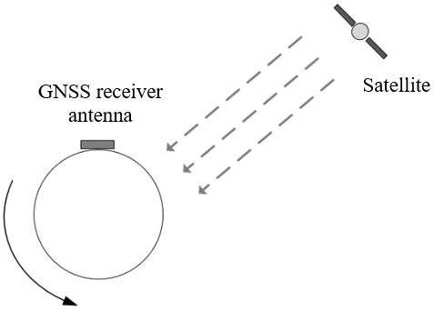
Figure 1. Geometric relationship between the single antenna and a satellite
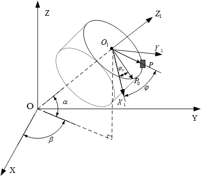
Figure 2. Geometric relationship between the ECEF coordinate system and the topocentric coordinate system
To estimate the roll rate of the cylindrical spinning vehicle by pseudorange observations, a single antenna of the GNSS receiver was mounted on the side of the vehicle. As the vehicle rotates, the pseudorange observations will oscillate in the form of a sine wave. The oscillation frequency is consistent with the vehicle roll rate. Therefore, the roll rate of the spinning vehicle can be estimated by analyzing the pseudorange observations. Figure 1 shows the geometric relationship between the single antenna and a satellite.
Figure 2 shows the relationship between the Earth-centered Earth-fixed (ECEF) coordinate system and the topocentric coordinate system $O_{1} X_{1} Y_{1} Z_{1}$.
In the topocentric coordinate system $O_{1} X_{1} Y_{1} Z_{1}$, the centroid of the vehicle serves as the origin $O_{1}$; the phase center of the non-omnidirectional antenna of the receiver lies the side point $P$ of the spinning vehicle, and its rotation plane is the cross-section of the vehicle. Once the vehicle starts rotating, the phase center of the antenna will run in the center of the circle, whose radius is r. The epoch of the circular motion of the antenna can be calculated by T=1/f, where $f$ is the vehicle rolling frequency. In Figure 2, $P_{0}$ and $\varphi_{0}$ are the initial position and initial phase of the circular motion of the antenna phase center, respectively.
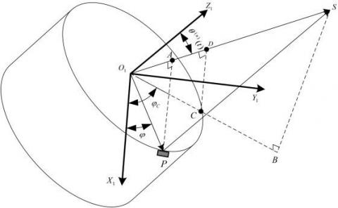
In each observation epoch, the GNSS receiver measures its geometric distance from the satellite based on the received signal. The measured distance is the pseudorange, including the clock differences of the satellites and the receiver, ionospheric delay, and troposphere delay. Figure 3 shows the analysis of pseudorange observations in the topocentric coordinate system, as the single antenna on the side of the vehicle rotates.
Figure 3. Antenna rotation vector and LOS vector
Note that $P$ is the phase center of the real-time antenna; $\overrightarrow{O_{1} P}$ is the rotation vector of the antenna, which corresponds to the real-time rolling phase of $\varphi(t)$; $|\overrightarrow{P S(n)}|$ is the distance between the antenna phase center and satellite n, namely, the real-time pseudorange observation $\rho^{(\mathrm{n})}(\mathrm{t}); \left|\overrightarrow{O_{1} S^{(n)}}\right|$ Qis the distance between the centroid of the vehicle and satellite n; $\overrightarrow{O_{1} A}$ is the projection of the rotation vector $\overrightarrow{O_{1} P}$ on the LOS vector $\overrightarrow{O_{1} S^{(n)}}$.
When the vehicle rotates, the rotation vector $\overrightarrow{O_{1} P}$ changes, $\left|\overrightarrow{O_{1} A}\right|$ would change with the real-time rolling phase $\varphi(t)$. If $\overrightarrow{O_{1} P}$ coincides with the projection $\overrightarrow{O_{1} B}$ of the LOS vector $\overrightarrow{O_{1} S^{(n)}}$ on plane $O_{1} X_{1} Y_{1}$, i.e., if $\overrightarrow{O_{1} P}$ rotates to $\overrightarrow{O_{1} C},\left|\overrightarrow{O_{1} A}\right|$ reaches the maximum. Let $\theta^{(\mathrm{n})}(\mathrm{t})$ be the angle between the normal vector $\overrightarrow{O_{1} Z_{1}}$ of the antenna rotation plane and the LOS vector $\overrightarrow{O_{1} S^{(n)}}$ of satellite n. Then, we have:
$\left|\overrightarrow{O_{1} A}\right|_{M A X}=\left|\overrightarrow{O_{1} C}\right| \cdot \sin \left[\theta^{(n)}(t)\right]$ (1)
where, $\left|\overrightarrow{O_{1} C}\right|=r$.
When the phase center of the antenna rotates with the vehicle, the $\overrightarrow{O_{1} C}$, which corresponds to the real-time rolling phase, can be described as $\varphi_{C}=2 \pi f t_{C}+\varphi_{0}$, where $t_{C}$ is the time required for the phase center of the antenna to rotate until it coincides with the projection $\overrightarrow{O_{1} B}$ of the LOS vector on plane $O_{1} X_{1} Y_{1}$. Thus, the real-time angle between $\overrightarrow{O_{1} P}$ and $\overrightarrow{O_{1} C}$ can be derived as:
$\begin{aligned} \varphi-\varphi_{C}=& 2 \pi f t+\varphi_{0}-\left(2 \pi f t_{C}+\varphi_{0}\right) \\ &=2 \pi f t-2 \pi f t_{C} \end{aligned}$ (2)
The real-time value of $\left|\overrightarrow{O_{1} A}\right|$ can be obtained from the angle:
$\left|\overrightarrow{O_{1} A}\right|=\left|\overrightarrow{O_{1} C}\right| \cdot \sin \left[\theta^{(n)}(t)\right] \cos \left(\varphi-\varphi_{C}\right)$
$\quad=r \cdot \sin \left[\theta^{(n)}(t)\right] \cos \left(2 \pi f t-2 \pi f t_{C}\right)$ (3)
Since $\left|\overrightarrow{O_{1} P}\right| \ll\left|\overrightarrow{P S^{(n)}}\right|,\left|\overrightarrow{O_{1} A}\right|$, the projection of $\overrightarrow{O_{1} P}$ on the LOS vector $\overrightarrow{O_{1} S^{(n)}}$, is negligible compared with $\left|\overrightarrow{O_{1} S^{(n)}}\right|$. Thus, we have $\left|\overrightarrow{A S^{(n)}}\right|=\left|\overrightarrow{P S^{(n)}}\right|$.
The time function $P_{m}(t)$ was designed to represent the time variation of real-time pseudorange observation $|\overrightarrow{P S(n)}|$; the time function $P_{L}(t)$ was designed to represent the time variation of real-time distance $\left|\overrightarrow{O_{1} S^{(n)}}\right|$ from vehicle centroid to satellite n; the time function $P_{S}(t)$ was designed to represent the time variation of real-time projection $\left|\overrightarrow{O_{1} A}\right|$ of rotating vector $\overrightarrow{O_{1} P}$ on LOS vector $\overrightarrow{O_{1} S^{(n)}}$:
$P_{\mathrm{m}}(t)=P_{L}(t)-P_{S}(t)=\left|\overrightarrow{P S^{(n)}}\right|$
$\quad=\left|\overrightarrow{A S^{(n)}}\right|=\left|\overrightarrow{O_{1} S^{(n)}}\right|-\left|\overrightarrow{O_{1} A}\right|$ (4)
According to formula (4), the pseudorange real-time observation $P_{m}(t)$ is composed of two parts: the first part $P_{L}(t)$ refers to the distance $\left|\overrightarrow{O_{1} S^{(n)}}\right|$ between vehicle centroid O1 and satellite n. It changes in real time due to the relative motion of vehicle and satellite; the other part $P_{S}(t)$ stands for the projection $\left|\overrightarrow{O_{1} A}\right|$ of the position vector $\overrightarrow{O_{1} P}$ on the LOS vector $\overrightarrow{O_{1} S^{(n)}}$, when the phase center of the receiver antenna rotates on the cross-section of the vehicle. This projection oscillates sinusoidally due to the circular motion of the receiver antenna, and the oscillation frequency is consistent with the rotation frequency of the vehicle. Meanwhile, the instantaneous value of $\left|\overrightarrow{\mathrm{O}_{1} A}\right|$ depends on the angle $\theta^{(n)}(t)$, which can be obtained from the normal vector $\overrightarrow{O_{1} Z_{1}}$ of the rotation plane, and the LOS vector $\overrightarrow{O_{1} S^{(n)}}$ of satellite n:
$\theta^{(n)}(t)=\operatorname{arcos} \frac{\overrightarrow{\mathrm{O}_{1} \mathrm{Z}_{1}} \cdot \overrightarrow{O_{1} S^{(n)}}}{\left|\overrightarrow{\mathrm{O}_{1} \mathrm{Z}_{1}}\right| \cdot\left|\overrightarrow{O_{1} S^{(n)}}\right|}$ (5)
When the vehicle moves in the air and the attack angle is zero, the normal vector of its rotation plane usually points to the direction of its speed. According to formula (5), the angle $\theta^{(n)}(t)$ changes with time due to vehicle motion.
Next, the vehicle motion was analyzed in powerless state. Since $P_{L}(t)$ refers to the distance $\left|\overrightarrow{O_{1} S^{(n)}}\right|$ between vehicle centroid O1 and satellite n, and changes in real time due to the relative motion of vehicle and satellite, we have:
$P_{L}(t)=P_{L}\left(t_{0}\right)+\left[\overrightarrow{V\left(t_{0}\right)}\left(t-t_{0}\right)+\overrightarrow{a(t)}\left(t-t_{0}\right)^{2}\right] \times \mathbf{H}$ (6)
where, $t_{0}$ is the initial moment of free fall for the powerless spinning vehicle after launch; t is any moment before the vehicle stops moving after $t_{0}; \mathrm{P}_{\mathrm{L}}\left(\mathrm{t}_{0}\right)$ is the initial pseudorange observation of the vehicle; $\overrightarrow{\mathrm{V}\left(\mathrm{t}_{0}\right)}$ is the initial speed vector of the vehicle; $\overrightarrow{a(t)}$ is the acceleration of the vehicle in free fall. In addition to the acceleration of gravity, the spinning vehicle may be affected by other factors, such as wind resistance in its free fall. Under the combined effect of these factors, the acceleration of the vehicle would change with time. This paper regards the variation in acceleration induced by factors except gravitational acceleration as the noise of pseudorange measurement. In addition, $\overrightarrow{a(t)}=\vec{a}$ is a constant vector consistent with the acceleration of gravity; $\mathbf{H}$ is the unit observation vector matrix. Let $s^{(n)}\left(x^{(n)}, y^{(n)}, z^{(n)}\right)$ be the coordinates of satellite n, and $P(x, y, z)$ be the coordinates of the antenna in topocentric coordinate system; $\rho^{(n)}(t)$ be the pseudorange observation between satellite n and the antenna. Then, we have:
$\mathbf{H}=\left[\begin{array}{l}\frac{\partial \rho^{(n)}}{\partial x} \\ \frac{\partial \rho^{(n)}}{\partial \mathrm{y}} \\ \frac{\partial \rho^{(n)}}{\partial \mathrm{z}}\end{array}\right]=\frac{\mathbf{1}}{\rho^{(n)}(t)}\left[\begin{array}{l}x-x^{(n)} \\ y-y^{(n)} \\ z-z^{(n)}\end{array}\right]$ (7)
Compared with the circular motion of the receiver antenna, matrix $\mathbf{H}$ can be regarded as a constant matrix in a very short period of observation epoch.
In formula (4), $P_{S}(t)$ is the projection $\overrightarrow{O_{1} P}$ on the LOS vector:
$P_{S}(t)=\left|\overrightarrow{O_{1} A}\right|=r \cdot \sin \left[\theta^{(n)}(t)\right] \cos \left(2 \pi f t-2 \pi f t_{C}\right)$ (8)
Substituting formula (5) into formula (8):
$P_{S}(t)=r \cdot \sin \left[\operatorname{arcos}\left(\frac{\overrightarrow{\mathrm{O}_{1} \mathrm{Z}_{1}} \cdot \overrightarrow{O_{1} S^{(n)}}}{\left|\overrightarrow{\mathrm{O}_{1} \mathrm{Z}_{1}}\right| \cdot\left|\overrightarrow{O_{1} S^{(n)}}\right|}\right)\right] \cos (2 \pi f t$
$\left.-2 \pi f t_{C}\right)$ (9)
The pseudorange observations between satellite n and the antenna can be obtained through baseband processing of GNSS signals. As can be seen from formula (6), $P_{L}(t)$, which is contained in the measured pseudorange, depends on the centroid of the vehicle, and the relative speed and acceleration of the satellite, but has nothing to do with the rolling of the vehicle. In other words, in a certain period, the change of $P_{L}(t)$ is the distance of relative motion between the vehicle centroid and the satellite, with the first-order component being the relative motion speed, and the second-order component being the relative motion acceleration. In the selected observation epoch, if the acceleration of the vehicle remains constant, the second-order component will be constant.
In the light of the pseudorange, satellite and receiver antenna positions, and the continuous differentiability of pseudorange during the vehicle’s free fall, the second derivative of formula (4) with respect to time t can be obtained:
$\frac{d P_{\mathrm{m}}(t)}{d t^{2}}=\frac{d P_{L}(t)}{d t^{2}}-\frac{d P_{S}(t)}{d t^{2}}$ (10)
During the free fall of the spinning vehicle, if only the influence of gravitational acceleration is considered, then $\overrightarrow{a(t)}=\vec{a}$ is a constant vector. Thus, we have:
$\frac{d P_{L}(t)}{d t^{2}}$
$=\frac{d\left\{P_{L}\left(t_{0}\right)+\left[\overrightarrow{V\left(t_{0}\right)}\left(t-t_{0}\right)+\overrightarrow{a(t)}\left(t-t_{0}\right)^{2}\right] \times \mathbf{H}\right\}}{d t^{2}}$
$=2(\overrightarrow{\boldsymbol{a}} \times \mathbf{H})$ (11)
$P_{S}(t)$ is only related to the vehicle’s rotational motion, with the first-order differential being the projection of the speed of the antenna ’s circular motion on the LOS vector, and the second-order differential being the projection of the acceleration of the circular motion on the LOS vector. Both differentials change in the form of a sine wave within the same frequency. Therefore, the roll rate of the vehicle can be calculated from the second-order differential of pseudorange observations $P_{m}(t)$:
$\frac{d P_{S}(t)}{d t^{2}}=r \cdot \sin \left[\operatorname{arcos}\left(\frac{\overrightarrow{\mathrm{O}_{1} \mathrm{Z}_{1}} \cdot \overrightarrow{O_{1} S^{(n)}}}{\left|\overrightarrow{\mathrm{O}_{1} \mathrm{Z}_{1}}\right| \cdot\left|\overrightarrow{O_{1} S^{(n)}}\right|}\right)\right] \cdot 4 \pi^{2} f^{2}$
$\cdot \cos \left(2 \pi f t-2 \pi f t_{C}\right)$ (12)
In the second-order differential of $P_{S}(t)$, the angle $\theta^{(n)}(t)$ is also a time-varying function, but its change rate is far less than that of pseudorange observation induced by the phase center rotation of antenna. Therefore, it is regarded as a constant in this research.
Formulas (10)-(12) show that, in the second-order differential of pseudorange observations, the part formed by the relative motion of the vehicle and the satellite (formula (11)) is a constant; the part formed by the rotational motion of the spinning vehicle (formula (12)) contains the alternating component with frequency f. This component can be obtained by subtracting the average of second-order differential of pseudorange observations. Then, the rotation frequency f of the spinning vehicle can be derived from the alternating component in the frequency domain.
According to formula (9), the alternating component is the projection of the real-time rotation vector $\overrightarrow{O_{1} P}$ on the LOS vector $\overrightarrow{O_{1} S^{(n)}}$ of satellite n. The vibration amplitude of the component is positively proportional to the angle $\theta^{(n)}(t)$ between the two vectors. The maximum possible vibration amplitude is the radius of the cylindrical spinning vehicle. During the flight of the spinning vehicle, the included angle $\theta^{(n)}(t)$ can be obtained by calculating the speed vector and the LOS vector. It is assumed that the attack angle of the spinning vehicle is zero during the flight, and the spinning axis of the vehicle is consistent with the speed vector.
The angle $\theta^{(n)}(t)$ is affected by the relationship between the cross-section and the LOS vector. To estimate the vehicle’s rotation frequency, the projection vibration amplitude of the rotation vector should be maximized to enlarge the corresponding spectral amplitude. Therefore, the angle $\theta^{(n)}(t)$ between the speed direction of the vehicle and the LOS vector needs to be calculated in real time. Then, the threshold $\theta_{T H}$ was set according to the change of the angle, and the measured pseudorange of the satellite $\theta^{(n)}(t)>\theta_{T H}$ was selected for estimating vehicle rotation speed. To suppress the interferences like the noise of pseudorange measurement, and wind resistance, the second-order differentials of pseudorange, whose angle $\theta^{(n)}(t)$ meets the requirements, were superimposed in the frequency domain to smooth the noise influence.
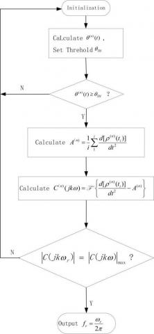
Figure 4 presents the overall structure of the spinning frequency estimation algorithm.
Figure 4. Flow chart of pseudorange-based spinning frequency estimation algorithm
In this paper, GNSS signals are baseband processed by the receiver during initialization phase to obtain real-time ephemeris, pseudorange, and Doppler frequency shift, and the least square method is employed to obtain the real-time speed vector of the antenna. The satellite position $s^{(n)}\left(x(t)^{(n)}, y(t)^{(n)}, z(t)^{(n)}\right)$, and receiver position $\left.O_{1}\left(x_{0}(t), y_{0}(t), z_{0}(t)\right)\right)$ were used to solve the LOS vector $\overrightarrow{O_{1} S^{(n)}}$, and then calculate the angle $\theta^{(n)}(t)$ between LOS vector $\overrightarrow{O_{1} S(n)}$ and speed vector $\overrightarrow{V\left(t_{0}\right)}$. The above analysis shows that the angle has a positive correlation with the spectral energy of the second-order differential of the pseudorange. Therefore, once the $\theta^{(n)}(t)$ of all visible satellites was calculated, the pseudorange observations were selected by the rule that $\theta^{(n)}(t)$ exceeds threshold $\theta_{T H}$. In epoches 1~i, the mean value $A^{(n)}$ of the second-order differential of $\theta^{(n)}(t)$ exceeds the threshold $\theta_{T H}$, which satisfy the above conditions, were solved. The i value was selected depending on the rotational period and signal sampling rate of the spinning vehicle.
In general, i should cover multiple epochs of the spinning vehicle. The more the covered epochs, the greater the spectral energy is obtained in the estimation of roll rate, and the more accurate the estimation of rolling frequency. Nevertheless, the number of epoch i must strike a balance between the real-timeliness of rolling frequency estimation, and the short constant period of matrix H. For each satellite in 1~i epochs, the mean value $A^{(n)}$ of the second-order differential of pseudorange was subtracted, leaving only the second-order differential of $P_{S}(t)$ shown in formula (11). The spectrum of the second-order differential of pseudorange was acquired by the FFT. Then, all the spectra of the second-order differentials of the pseudorange meeting the threshold $\theta_{T H}$ were added up, and the maximum of the sum $|C(j k \omega)|_{\max }$ was identified. Finally, the frequency point $\omega_{r}$ corresponding to the maximum spectrum $|C(j k \omega)|_{\max }$ was solved, and the estimated vehicle rolling frequency was outputted as $f_{r}=\frac{\omega_{r}}{2 \pi}$.
To verify the correctness of our algorithm, computer simulations were carried out to generate satellite ephemeris and receiver data. In the generated data, the diameter of the spinning vehicle is 155mm, the noise of pseudorange measurement is Gaussian white noise with a mean of zero, and a standard deviation of σ: $\mathrm{N}\left(0, \sigma^{2}\right)$. Empirical results show that the standard deviation $\sigma$ is less than 1m. This paper sets $\sigma \in[0,5]$.
Three motion states of the vehicle were simulated. In state 1, the vehicle moved uniformly with spinning. In state 2, the vehicle decelerated uniformly with spinning. In state 3, the vehicle first accelerated and then decreased uniformly, always with spinning. The pseudorange observations were sampled at 50Hz. The number of observed epochs surpasses 1,000. A 4,096-point FFT was used in the simulations.
The simulation approach involves the following steps:
Step 1. Set the motion state and pseudorange sampling frequency in the GNSS signal analog source, and output the pseudorange observations and Doppler frequency shift measurements in each epoch.
Step 2. Based on the output data from Step 1, calculate the real-time position and speed of the receiver antenna, the LOS vector $\overrightarrow{O_{1} S(n)}$, and speed vector $\overrightarrow{V\left(t_{0}\right)}$, and then derive the angle $\theta^{(n)}(t)$.
Step 3. Set the threshold $\theta_{T H}$ by experience, and compare $\theta^{(n)}(t)$ with the threshold. If $\theta^{(n)}(t)$ is greater than the threshold, retain the corresponding pseudorange observations $\rho^{(\mathrm{n})}(\mathrm{t})$ for further analysis.
Step 4. Compute the mean second-order differential of the corresponding pseudorange observations.
Step 5. Subtract the mean $A^{(n)}$, and calculate the spectra of the second-order differentials of the corresponding pseudorange observations.
Step 6. Find the maximum of the spectrum, and output the corresponding frequency point $f_{r}$, i.e., the vehicle rolling frequency.
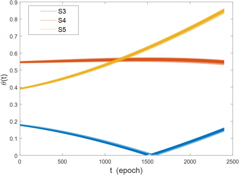
The performance of our algorithm was analyzed under different noises of pseudorange measurements. The LOS vector and speed vector of satellites No. 3, No. 4, and No. 5 were observed under the three different states above, and used to solve the variation of angle $\theta^{(n)}(t)$ within 2,400 epochs.
Figure 5. The angle $\theta^{(n)}(t)$ between the LOS vector $\overrightarrow{O_{1} S(n)}$ and speed vector $\overrightarrow{O_{1} S^{(n)}}$
As illustrated in Figure 5, the angle $\theta^{(n)}(t)$ between the LOS vector and speed vector (rotation axis vector of the vehicle) of three satellites presented different features. During the observation epochs, the angle $\theta^{(n)}(t)$ corresponding to satellite No. 3 was the smallest, that corresponding to satellite No. 4 remained at $\frac{\pi}{6}$, and that corresponding to satellite No. 5 rose from $\frac{\pi}{8}$ to $\frac{2 \pi}{7}$.
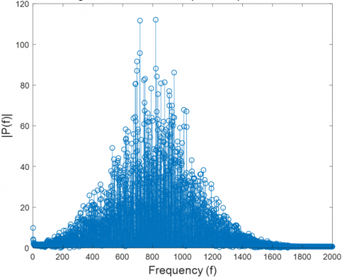
Figure 6 shows the second-order differential spectrum of pseudorange observations obtained by the receiver corresponding to each of the three satellites, when the vehicle roll rate was 10r/s. It can be observed that, large value points of the spectrum appeared at the rolling frequency of 10Hz, and the noise of other frequencies was contained in the spectrum due to the noise of pseudorange observations. However, the difference between this frequency point and other frequency points in terms of the amplitude of the frequency spectrum depends on the angle that directly affects the recognition of the rolling frequency of the vehicle.
In the second-order differential $P_{S}(t)$ specturm for the pseudorange observation corresponding to satellite No. 3, the spectral curve peaked at frequency point 820 ($f_{r}=\frac{\text { sample rate } \times \text { number of frequence }}{\text { number of } F F T}=\frac{50 \times 820}{4096}=10.00 \mathrm{~Hz}$), but the second-highest peak appeared at frequency point 715 ($f_{r}=8.72 \mathrm{~Hz}$), where the amplitude is very close to the peak amplitude. A slight change to the measurement error will cause incorrect identification of the peak frequency point. Consistent with the preorder analysis, in the second-order differential spectrum of the pseudorange observation of satellite No. 3, the projection of the rotation vector on the LOS vector fluctuated with a small amplitude, which hinders the identification of vehicle rolling frequency.
(a) Second-order differential spectrum of pseudorange observations corresponding to satellite No. 3
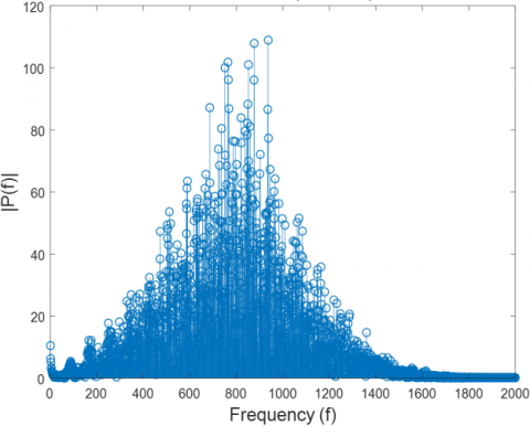
(b) Second-order differential spectrum of pseudorange observations corresponding to satellite No. 4
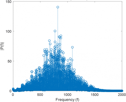
(c) Second-order differential spectrum of pseudorange observations corresponding to satellite No. 5
Figure 6. Spectrum of second-order differentials of pseudorange observations corresponding to the three satellites
Similar results can be obtained from the second-order differential $P_{S}(t)$ specturm for the pseudorange observation corresponding to satellite No. 4. When it comes to the second-order differential $P_{S}(t)$ specturm for the pseudorange observation corresponding to satellite No. 5, however, the spectrum peaked at frequency point 820, while the spectral amplitude of other frequency components was relatively small. Therefore, the main frequency component in the signal could be accurately identified by the spectral peak: the vehicle rolling frequency was 10.00Hz.
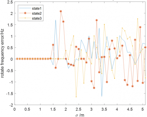
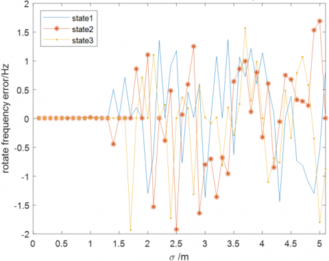
(a) Frequency identification error at roll rate 3r/s
(b) Frequency identification error at roll rate 10r/s
(c) Frequency identification error at roll rate 20r/s
Figure 7. Estimation results of vehicle rotation frequency under different errors of pseudorange measurement
Through the above analysis, the second-order differential spectrum of the pseudorange observation has a spectrum component related to the rotation frequency. Thus, it is possible to identify the vehicle rotation frequency using the spectrum. It can be learned from the second-order differential spectrum of the pseudorange observations of the three satellites that: With a large angle $\theta^{(n)}(t)$ between the LOS vector and speed vector, satellite No. 5 can identify the spectral peak point corresponding to vehicle rolling frequency more accurately than the other two satellites.
Furthermore, several experiments were conducted with different rotation speeds to analyze the performance of the roll rate estimation method. The experimental results are displayed in Figure 7.
The roll rates were estimated under the spinning vehicle speed of at 3r/s, 10r/s, and 20r/s, respectively. For pseudorange measurement noise, the standard deviation should fall in the range of $0 m \leq \sigma \leq 5 m$. As shown in Figure 7, our method could accurately estimate the roll rate when the standard deviations of pseudorange measurement noise were less than 1m. The estimation accuracy decreased, after the standard deviations reached and surpassed 1m. In practical application, the standard deviation of pseudorange observation noise in GNSS systems, such as GPS and the BeiDou Navigation Satellite System (BDS), is less than 0.4m. The pseudorange measurement noise can be further reduced through proper optimization. Hence, our approach is suitable for estimating the rotation speed of the cylindrical spinning vehicle in GNSS systems.
This paper proposes an estimation approach for the roll rate of the highly dynamic cylindrical spinning vehicle based on real-time pseudorange observations. Firstly, a single antenna was mounted on the side of the cylindrical spinning vehicle to receive GNSS signals. Then, the second-order differential of pseudorange was calculated. Assuming that the acceleration of the aircraft remains constant, the second-order differential of pseudorange would vary in the form of a sine curve. Then, the features of the frequency domain were analyzed. The roll rate of the cylindrical spinning vehicle was identified after extracting the peak of the spectrum. In addition, three vehicles with different roll rates were simulated and tested. The results show that the roll rate of cylindrical spinning vehicle can be accurately identified when the pseudorange measurement noise is less than 1m, which is suitable for the current mainstream GNSS systems. The main contributions of this paper are as follows:
Our approach estimates the rolling frequency of the vehicle based on the signals received by a single antenna of GNSS receiver. Compared with the multi-antenna mode, our approach reduces structural complexity, and weakens signal interference between antennas. Besides, the required pseudorange observations can be obtained through the pseudo-random code tracking loop, which is more robust, and less computationally intensive than the traditional carrier tracking loop. Moreover, the quantity of pseudorange observations is the conventional output of GNSS receiver. Our approach requires no customization, which is necessary in traditional schemes, which identify the rolling frequency according to the signal amplitude received by the customized receiver. The elimination of customization further reduces the cost of attitude measurement devices, and ensures the simplicity and lightweight of the algorithm.
This work is supported by the National Natural Science Foundation of China (Grant No.: 52077011), Youth Project of National Natural Science Foundation of China (Grant No.: 42001297), Major Project of Changsha Science and Technology Bureau, 2020 (Grant No.: kq2011001), and Key Research and Development Project of Science and Technology Department of Hunan Province, 2022 (Grant No.: 2022GK2026).
[1] Park, J.I., Yoon, J.Y., Kim, D.S., Yi, K.S. (2008). Roll state estimator for rollover mitigation control. Proceedings of the Institution of Mechanical Engineers, Part D: Journal of Automobile Engineering, 222(8): 1289-1312. https://doi.org/10.1243/09544070JAUTO803
[2] García-Fernández, M., Markgraf, M., Montenbruck, O. (2008). Spin rate estimation of sounding rockets using GPS wind-up. GPS Solutions, 12(3): 155-161. https://doi.org/10.1007/s10291-007-0074-8
[3] Lee, H.S., Park, H., Kim, K., Lee, J.G., Park, C.G. (2008). Roll angle estimation for smart munitions under GPS jamming environment. IFAC Proceedings Volumes, 41(2): 9499-9504. https://doi.org/10.3182/20080706-5-kr-1001.01606
[4] Lee, S.H., Ahn, H.S., Yong, K.L. (2009). Three-axis attitude determination using incomplete vector observations. Acta Astronautica, 65(7-8): 1089-1093. https://doi.org/10.1016/j.actaastro.2009.03.018
[5] Lee, J.Y., Kim, H.S., Choi, K.H., Lim, J., Chun, S., Lee, H.K. (2016). Adaptive GPS/INS integration for relative navigation. GPS solutions, 20(1): 63-75. https://doi.org/10.1007/s10291-015-0446-4
[6] Maus, S. (2008). The geomagnetic power spectrum. Geophysical Journal International, 174(1): 135-142. https://doi.org/10.1111/j.1365-246X.2008.03820.x
[7] Knight, J., Hatch, R. (1991). Attitude determination via GPS. Kinematic Systems in Geodesy, Surveying, and Remote Sensing, New York, US, pp. 168-177. https://doi.org/10.1007/978-1-4612-3102-8_16
[8] Wang, X., Yao, Y., Xu, C., Zhao, Y., Zhang, H. (2021). An improved single-epoch attitude determination method for low-cost single-frequency GNSS receivers. Remote Sensing, 13(14): 2746. https://doi.org/10.3390/rs13142746
[9] Chang, L., Qin, F., Li, A. (2014). A novel backtracking scheme for attitude determination-based initial alignment. IEEE Transactions on Automation Science and Engineering, 12(1): 384-390. https://doi.org/10.1109/TASE.2014.2346581
[10] Giorgi, G., Teunissen, P.J., Gourlay, T.P. (2012). Instantaneous global navigation satellite system (GNSS)-based attitude determination for maritime applications. IEEE Journal of Oceanic Engineering, 37(3):348-362. https://doi.org/10.1109/JOE.2012.2191996
[11] Leite, N.O., Walter, F. (2007). Flight test evaluation of a new GPS attitude determination algorithm. IEEE Aerospace and Electronic Systems Magazine, 22(12): 3-10. https://doi.org/10.1109/MAES.2007.4408595
[12] Hide, C., Pinchin, J., Park, D. (2007). Development of a low cost multiple GPS antenna attitude system. In Proceedings of the 20th International Technical Meeting of the Satellite Division of the Institute of Navigation (ION GNSS 2007), Fort Worth, TX, pp. 88-95.
[13] Doty, J.H., Anderson, D.A., Bybee, T.D. (2004). A demonstration of advanced spinning-vehicle navigation. In Proceedings of the 2004 National Technical Meeting of the Institute of Navigation, San Diego, CA, pp. 573-584.
[14] Doty, J.H., McGraw, G.A. (2003). U.S. Patent No. 6,520,448. Washington, DC: U.S. Patent and Trademark Office.
[15] Wierzbicki, D., Krasuski, K. (2015). Estimation of rotation angles based on GPS data from a UX5 Platform. Measurement Automation Monitoring, 61(11): 516-520.
[16] Jang, J., Kee, C. (2009). Verification of a real-time attitude determination algorithm through development of 48-channel GPS attitude receiver hardware. The Journal of Navigation, 62(3): 397-410. https://doi.org/10.1017/S0373463309005384
[17] Deng, Z., Shen, Q., Deng, Z. (2018). Roll angle measurement for a spinning vehicle based on GPS signals received by a single-patch antenna. Sensors, 18(10): 3479. https://doi.org/10.3390/s18103479
[18] Nguyen, B.M., Wang, Y., Fujimoto, H., Hori, Y. (2013). Advanced multi-rate Kalman filter for double layer state estimator of electric vehicle based on single antenna GPS and dynamic sensors. IFAC Proceedings Volumes, 46(5): 437-444. https://doi.org/10.3182/20130410-3-CN-2034.00015
[19] Zeng, G.Y. (2015). Navigation and roll atttidude determination technology by non-omnidirectional antenna under rotation condition. Doctor Thesis, Beijing Institute of Technology.
[20] Liu, Y., Li, H., Du, X. (2019). Roll attitude measurement technique based on GPS signal power. In 2019 IEEE International Conference on Unmanned Systems (ICUS), Beijing, China, pp. 280-284. https://doi.org/10.1109/ICUS48101.2019.8995938
[21] Kim, J.W., Cho, J.C., Hwang, D.H., Lee, S.J. (2008). A Roll rate estimation method using GNSS signals for spinning vehicles. Journal of Institute of Control, Robotics and Systems, 14(7): 689-694. https://doi.org/10.5302/J.ICROS.2008.14.7.689
[22] Lee, S., Jin, M., Choi, H.H., Lee, S.J. (2016). Design of roll rate estimator using GPS signal for spinning vehicle. Journal of Positioning, Navigation, and Timing, 5(3): 109-118. https://doi.org/10.11003/JPNT.2016.5.3.109
[23] Gan, Y., Sui, L., Xiao, G., Zhang, Q., Wang, L. (2021). Real-time GNSS attitude determination by a direct approach with efficiency and robustness. Measurement Science and Technology, 32(11): 115904. https://doi.org/10.1088/1361-6501/ac18a4
[24] Bevly, D.M., Gerdes, J.C., Wilson, C. (2002). The use of GPS based velocity measurements for measurement of sideslip and wheel slip. Vehicle System Dynamics, 38(2): 127-147. https://doi.org/10.1076/vesd.38.2.127.5619