Feroz Morab* | Rajeshwari Hegde | Veena N. Hegde
© 2022 IIETA. This article is published by IIETA and is licensed under the CC BY 4.0 license (http://creativecommons.org/licenses/by/4.0/).
OPEN ACCESS
The Electromagnetic (EM) waves are impinging on the base station from all the directions, Equally Spaced Uniform Linear Antenna Array (ESULA) are used to process these incoming EM waves to Detect and Estimate the directions of the mobile transmitters. After the process of Detection and Estimation, Electronic Beamforming is used to provide the narrow sharper beam towards the detected user. This Detection, Estimation and Beamforming plays a key role in variety of use cases like Radar, Wireless Communication and Sonar based systems. Smart Antenna Systems are implemented using two strategies namely Direction of Arrival (DoA) and Beamforming (BF). Direction of Arrival is a mechanism of Detecting and Estimating the directions of the mobile transmitters. Beamforming on the other hand is a process of transmission of the EM waves towards the source in a specific direction and providing the Spectral Nulls to other Interfering users. To increase the user capacity and to enhance the user experience Spatial Location based Spatial Division Multiple Access (SDMA) technology is used. To improve the overall performance of the smart antenna systems energy and packet delivery is majorly focused on specific source directions rather than using blind transmission strategy. In this paper performance analysis of algorithms for Direction of Arrival methods as well as the Beamforming methods have been performed. Experimental simulations are conducted and comparison is done with respect to Bias, Resolution and Time complexity for the Direction of Arrival methods. Noise Subspace Method (NSM) DoA algorithm consistently delivered the optimal bias, high resolution detection of the user location in spatial domain and provided lesser time complexity for both the scenarios which uses fewer antenna elements or larger number of antenna array elements at the base station. Similarly for the case of Beamforming methods the Mean Square Error and Beam-directions have been compared.
smart antennas, DoA, beamforming, phased antenna array, 5G, adaptive array antennas, array signal processing
In the legacy system the base station generally makes use of either parabolic dish or a horn antenna in order to send the signal towards the desired source, the efficiency of data transmission is low as each source uses different operating frequency [1]. Hence if there are ten users in the ecosystem then ten different frequencies are applied. As the number of users increases the capacity decreases, the improvement can be made by re-using the same frequency at different time.
This will increase the value of capacity to accommodate users within the same frequency band but has the limitation of latency. With the advent of spatial based systems it has to be noted that by making use of same frequency at the same time different beams can be radiated towards the users provided they are spatially separated.
Smart Antenna System combines two different processing strategies at the base station namely Detection Method and Radiation Formation Method. During Reception Phase, the incoming electromagnetic message signals are processed at the base station (BS) to perform the detection of the desired users location and during Transmission Phase; the Phase-Shifts are computed and applied to the antenna array elements in order to form the main beam towards the desired users and spectral nulls towards the interfering users.
Figure 1. Smart Antenna System
The Figure 1 shows the Set-up of Smart Antenna System which comprises a sequence of antenna array elements which are equally spaced from each other. Each of the antenna elements are connected to the Duplexer and Down Converter (D\C), the incoming electromagnetic message signals are always high frequency signals, which were upconverted during their transmission stage, the Down Converter (D\C) down coverts the high frequency signals and passes them to the Analog to Digital Converter (ADC) system. All the natural signals which are either transmitted or received are analog in nature, thus to perform the digital signal processing there is a need to convert analog signals to digital signals. This conversion task is carried out by the Analog to Digital Converter (ADC) system. Smart Antenna System makes use of Adaptive Mechanism, which takes these incoming digitized electromagnetic signals processes them and then generate the Weight Vector values, which are indeed attached to each antenna elements. This will produce a radiation, which forms the main beam towards the end user, unlike traditional beamforming in which antenna elements have fixed weights as an input.
The smart antenna based system will compute the weights based on the condition of the electromagnetic waves hitting the base station and appreciatively adjust the weight values.
There is an increasing demand for higher data rate, lower latency, more internet based mobile services bio detection applications, to fulfill these needs an efficient use of spectrum is need. This need can be fulfilled by the use of smart antenna system where energy and packet delivery is majorly focused on specific source directions rather than using blind transmission strategy.
The estimation of source directions is done using steering vector, which is extracted from actual signal along with the delayed version of same signal to have better efficiency. The detection of directions is labeled as baseline or subspace detection depending upon how the power spectrum is computed. The advantage of subspace is that it will have good resolution as well as lower amount of bias. Bias is a Performance Parameter of the Smart Antenna System, which informs the system about what was the Estimated Direction to the Actual Direction of the desire user Bias = |θEstimated – θActual|.
There are multiple ways in which the desired signal can be extracted due to the usage of multiple antenna elements at the base station. The first approach combines the original signal along with delayed version of the same signal. The second approach is used to select one of the signals which has high Signal to Noise Ration (SNR) among all the antenna elements. The first approach is termed as Maximal Ratio Combining and second approach is Diversity Combining.
The paper is organized as follows: Section II describes the Background. The design of proposed Direction of Arrival algorithm is discussed in Section III. Section IV deals with Beamforming algorithms. Experimental simulation results are presented in the Section V. Finally, Section VI Concludes the paper.
The incoming Electromagnetic signals are taken, amplitude computation is done along with phase vector computation, the advantage of using amplitude-based detection is that the computed direction will be more accurate. To further enhance the detection accuracy, the base station can implement the multi beam based uniformly excited linear antenna array arrangement [2].
The detection of sources underwater is done first computing the covariance matrix. The covariance matrix not only contains signal but also contains information on ambient noise. The subspace matrix is computed after finding out the eigenvalues, filtering them based on magnitude and then obtaining the lowest eigenvalues to get the noise space matrix. Ambient Noise Elimination is responsible for transforming the matrix to have lower noise magnitude with the help of Singular Value Decomposition (SVD) [3].
Direction of Arrival of a wideband acoustic signal is estimated using the maximal eigen-gap estimator which uses a single sensor vector. Computation of narrowband cross spectral density matrices are obtained by combining the optimal weights which produce signal subspaces which gives rise to maximal eigen-gap estimator. The detection scheme obtains the direction of the acoustic signal falling on the base station, it then performs the computation of cross-spectral density to find the optimal phase shifts. These phase shifts are then used for the radiation generation and data transmission. The Power Spectrum is computed using the Eigen-gap estimator which detects the directions of sources [4].
The source detection is done by computing the Discrete Fourier transform (DFT). Total Least Squares (TLS) is computed by making use of offsets values which perform execution of Taylor equation in order to reduce the noise value [5].
Hydro-acoustics and aeronautics applications also require the detection of sources. The closed-form equation of Cramer- Rao bound is used to detect the sources by making use of antenna used for measuring the attitude. The Gaussian noise is computed along with signal matrix in order to compute a real environment detection of directions [6].
The different variation of co-variance matrix is computed known as Augmented Co-Variance matrix. The argument matrix computation is done in order to reduce the noise effect using rank based minimization. The arrangement of antenna elements is done into two separate prime arrays with each array having the determination of directions of sources [7].
The spatial domain based system increases the capacity of communication model. If we make use of single element at the base station then we have no choice except to process the signal from the sources which are having higher signal strength but when we have an array of elements then we have signal along with them we have delayed version of the same signal so that the detection capacity is improved even if the signal is weak. The value of array manifold vector is computed in a linear fashion by making use of Bayesian learning (SBL). Size and computational complexity are the factors used for detection of direction based on likelihood functionality [8].
The detection of directions for the sources is done based on amplitude computation, the eigenvectors are found out for the correlation matrix. The eigenvalues for the correlation matrix are computed and then arranged in a descending order. If there are N antenna elements then N-Nsources value is computed where Nsources are the number of users to be detected. Once those are computed the subspace matrix is determined and then compute the power spectrum for detecting the sources [9].
Hybrid-ADC is used for multi user massive MIMO systems, which computes the spatial covariance matrix which forms the power spectrum using MUSIC method. The group of independent detection arrays are used which form the linear equations containing both the amplitude and directions from the sources. Detection, Estimation and Location is done on the basis of noise subspace [10].
The Bayesian inference method computes the detection for algorithms, IMUSIC method will compute the weight vector based on spatial computation using grid model and computation of steering vector using Taylor method [11].
This array is divided into two sections. The first section makes use of conjugate value and second section will perform the difference between signal amplitude values [12]. Amplitude and phase entities are computed from each of antenna elements. Lower Cost and bandwidth computations are achieved in order to perform the correlation between actual signal hitting the base station and its Hermitian transpose. Multi beams weights are computed and then radiation is formed on each source independently [13].
The measure of pressure and velocity are computed in order to determine the direction of sources. The detection process methods are divided into multiple types. The combination of histogram along with intensity computation is used for likelihood based methods. In the second type subspace is computed over the co-variance matrix in order to determine the directions of sources. The capability of the algorithms to determine the sources which are closely separated into distinct directions is better for second type as compared to first type [14]. The compressive based sensing is responsible for first detecting the direction of sources. Combination of beam space techniques are used for detection of single and multiple directions [15].
The computation of magnitude along with subspace matrix is constructed to derive the Power Spectrum, which uses the Co-Array MUSIC-Group Delay (Co-Array MGD) algorithm. This Co-Array MGD Algorithm is generated by forming a Product of Co-Array MUSIC Magnitude and Co-Array Group Delay Function. The Co-Array Group Delay Function is obtained by taking the negative differentials of the phases, this enables the effective detection of the closely-spaced sources in the spatial domain [16].
Long Term Evolution (LWA) array will execute the beam-forming on the applications which are used for indoor as well mobile based communication. The array is created using a feeding element along with four port based SIW. Different beam directions are determined by making use of phase shifts and then weights are attached to individual element in order to determine the directions of sources [17].
The detection of directions involves sequence of steps, the first step is to compute the steering vector followed by amplitude computation. The computation of array correlation matrix is done combining both signal impinging on the antenna elements and noise signals. The eigenvalues are computed and then decrease in the value of Eigen are performed in the sorted order. After that the eigenvectors are found for those eigenvalues and then noise subspace is found to detect the directions of signal. The beam-forming is done by computing the steering vectors, finding the mean square error along with step size in order to compute the phase shifts which can be applied to individual antenna elements and then form the main beam towards the radiation formation [18].
The channel state information (CSI) is computed by making use of antenna elements which can be applied to individual element in order to compute the phase shifts. The training data is first generated from the mobile signal that will be pure signal. The steering vector is computed for the pure signal direction along with other interference vector directions. The next step is to compute the error signal, compute the step size and finally the phase shift is applied to individual antenna element to form the main beam and side lobes towards the interference directions [19].
The communication is performed by making use of duplex approach at the base station. During the reception the antenna elements are used to receive the electromagnetic waves and process the waves in order to detect the directions. During the transmission phase the phase shifts are computed and then applied to individual antenna elements to form the beam and side lobes. The uplink transmission happens from the mobile source towards the base station. During the downlink process the transmission of data from the base station to the mobile source [20].
The antenna elements are arranged in a linear fashion with each element equally spaced between antenna elements. The phase shift vectors are computed by making use of previous phase shifts, step size, error computation along with phase shifts. The phase shifts are computed based on the value of maximum signal to noise ratio (SNR). The fading is computed based on gamma variables and then chi square computation is done to compute the updated values of weights. The weights are computed in order to form the main beam towards the source and then side lobes towards interference users [21].
The antenna will be configured in a smart and rewire elements configuration. The signal coming from sources are hopped on multi other elements and then send towards the base station. The relay based antenna elements can be used in middle in order to perform the reflection of transmitted beam so that it can be reflected towards the mobile user [22].
The detection of the desired users in the spatial domain is obtained by computing the Power Spectrum, wherever the peaks arises it denotes the location of the desired user. Thus the computation of Power Spectrum is done in multiple steps such as: The First step is to compute the steering vector in a specific direction, the Second step is to steer the beam towards the source. The accuracy is increased by making use of minimum variance distortion-less response, the pattern synthesis focuses on computing the phase shifts, which can be applied to individual antenna elements. The Peaks of the Power Spectrum represent the detection of the desired users in the spatial domain [23].
The estimation of angles for the mobile sources by performing the amplitude computation as well as phase computation. There are multiple ways in which phase shifts computation can happen based on either amplitude peak detection or correlation based method then phase shift will get applied to individual antenna elements [24]. The elements are arranged in a linear fashion with each element spaced at an equal distance The phase shifts are computed in such a way that main beam is formed towards the actual source direction and then side lobe radiation is formed towards the unwanted directions. Comparison of algorithms are done based on computation of mean square error values and NLMS has the low error [25].
The elements are arranged in a uniform linear array (ULA) fashion. There is an error due to difference obtained between original signal and signal received at the base station and the error can be reduced by making use of MVDR based processing [26].
Long Term Evolution (LTE) along with Wimax technology are responsible for making use of beam formation process by applying the phase shifts to individual elements. The generation of main beam in a specific direction is done based on phase shifts which have been applied. Beam Division Multiple Access (BDMA) is used to form the beam towards the source by applying the phase shifts to antenna elements [27].
The beam-forming based co-efficient are computed by making use of Capon spatial spectrum Signal by computing the co- variance matrix which contains the steering vector of all the directions where sources are available. The phase shifts are computed and then applied to each of the antenna elements in order to form the main beam towards the desired user direction and have side lobe towards the interference direction [28].
Digital based phase shifts are computed in an adaptive fashion and then applied to the individual antenna elements. Classic approach makes use of library of weights which does not take into consideration the noise present in electromagnetic wave as well as noise present within the antenna elements. The adaptive approach will take the noise also into consideration and then adjust them to take of cancellation of interference [29].
The beam which are narrow in nature towards the source can be utilized for larger amount of data transfer. The steering of beam across the directions at mmWave frequencies help in finding the location of resource and then follow the resource by applying dynamic phase shift based on changing location of the resource. Bayesian method which can predict the mobility nature of the resource and then target the beam towards detection of resource [30]. The transmission of data in the Sensing Data Network consists of base station (BS) which makes use of array of antenna elements there by increasing the throughput in the entire area. Energy Source along with hybrid based system is used to apply the phase shifts to the individual antenna elements [31].
The Direction of Arrival (DoA) algorithms are responsible for detecting the directions of the sources, the DoA algorithms are classified as Conventional Methods and Subspace Methods. In the Conventional Methods, the detection of the users is directly computed by finding the Power Spectrum without performing any complex signal processing techniques.
For the Subspace Methods, the detection of the users is determined by generating the Subspaces which act like Basis Functions, which enables to perform complex signal processing techniques to get optimal Bias and High Resolution Detection.
3.1 Total Correlation Detection Method (TCD)
The Total Correlation Detection Method will find the auto- correlation of the signal amplitudes along with its Hermitian Transpose. The auto-correlation vector is then used in the power spectrum to form the spectrum ranging from -90 to 90 and then the directions in which peaks are maximum are the detected directions.
$\begin{aligned}
&S P_{T C D M}=\frac{E M S v^{H}(\theta) S C E M S v(\theta)}{N_{e l e}^{2}}\\
&\text { Where, }\\
&E M S v(\theta)=\text { directionvectorforanangle } \theta\\
&E M S v^{H}(\theta)=\text { hermitiantransposeofdirectionvector }\\
&S C=\text { signalcorrelationmatrix }\\
&N_{\text {ele }}=\text { NumberofElements }
\end{aligned}$ (1)
3.2 Lang and McClellan Method (LANG)
Lang and McClellan will find the co-relation matrix. From each of the columns of the co-relation matrix the column which has the highest magnitude is chosen as the maximum vector.
$P_{L M M}=\frac{1}{E M S v(\theta)^{H} M C_{C} M C_{C}^{H} E M S_{v}(\theta)}$
Where,
$E M S v(\theta)^{H}$=hermitiantransposefordirectionvector
$E M S_{v}(\theta)=$ directionvector
$M C_{C}=M$ MximumCo - relation
$M C_{C}^{H}=$ hermitianMaximumCo - relation (2)
3.3 Correlation Inverse Likelihood (CIL)
Each time during the detection of the directions only one direction is treated as the direction and other directions are treated as belonging to disturbance. The inverse of co-relation matrix is used for the computation of power spectrum.
$P S_{C I L}=\frac{1}{E M S v^{H}(\theta) T S N C_{i n v} \operatorname{EMSv}(\theta)}$
where,
$E M S v^{H}(\theta)=$ hermitiantransposeofdirectionvector
$E M S v(\theta)=$ directionvector
$T S N C_{i n v}=$ computinginversefortotal
co - relationmatrix (3)
3.4 Noise Subspace Method (NSM)
The electromagnetic waves which are incident on the array elements get a multiple version with first original signal hitting the first antenna element along with them delayed versions of the same electromagnetic wave at each subsequent antenna elements. The signal correlation matrix is computed along with Hermitian transpose of correlation matrix. The eigenvalues of the correlation matrix are found and then the eigenvalues are arranged in the ascending order by taking first number of sources. For each of the eigen values eigenvector is found and combined to form noise vector space and then power spectrum is computed.
$P S_{C I L}=\frac{1}{E M S v^{H}(\theta) N S * N S_{i n v} E M S v(\theta)}$
where,
$E M S v^{H}(\theta)=$ hermitiantransposeofdirectionvector
$E M S v(\theta)=$ directionvector
$N S=$ noisesubspace
$N S_{i n v}=$ noisesubspaceinverse (4)
The emitting signals from the antenna elements produce main radiation, side lobes for disturbance signal and null values. All the elements are spaced at equal intervals with a spacing of distance (d). The main radiation is formed towards the actual direction of mobile with side lobes towards disturbance. The beam is shifted in different directions with phase shifts applied to each antenna elements.
The antenna elements used in the base station are attached to individual array elements with each element applied with a phase vector which is computed based on incoming electromagnetic waves along with noise vector. The phase vector must be computed in an intelligent manner with the help of a software algorithm which can be embedded on a device present at the base station.
4.1 Weighted Linear Method (WLM)
The phase shifts are computed and used in the communication based use cases. The algorithm is robust in nature along with low complexity value. During the computation of weight vector the training signal knowledge is important for computation of phase shifts. The phase shifts are computed using the following.
$P S_{W L}(k+1)=P S_{W L}(k)+$
$\frac{A C i n v * E M S_{v}(\theta)}{E M S v^{H}(\theta) * A C_{i n v} * E M S_{v}(\theta)}$
$+\sum_{k=1}^{N_{\text {disturb }}} \frac{A \operatorname{Cinv} * E M S_{v}\left(\theta_{k}\right)}{E M S v^{H}\left(\theta_{k}\right) * A C_{i n v} * E M S_{v}\left(\theta_{k}\right)}$
Where,
$P S_{W L}(k)=$ previousphaseshifts
$P S_{W L}(k+1)=$ phaseshiftsofnextiteration
$E M S_{v}(\theta)=$ directionalvector
$E M S v^{H}(\theta)=$ inversefordirectionalvector
$A C_{i n v}=c o-$ relationinverse
$N_{\text {disturb }}=$ numberofdisturbances
$E M S_{v}\left(\theta_{k}\right)$=directionalvectorforkthdisturbance $\theta_{k}$
$E M S v^{H}\left(\theta_{k}\right)=$hermitiantransposeforEM $S_{v}\left(\theta_{k}\right)$ (5)
4.2 Widely Linear Conjugate Gradient Method (WLCG)
$w p s(k+1)=\left[w p s^{T}(k) * w p s^{H}(k)\right]^{T}$
Where,
$w p s(k)=\frac{\text { Where }}{2 R\left\{E M S^{H}\left(\theta_{o}\right) * v v(k)\right\}}$
$v v(k)=v v(k-1)+\alpha w(k) * p w k(k)$
$\alpha w(k)=\frac{R\left\{g w_{k}^{H}(k-1)+p w k(k-1)\right\}}{R\left\{p w_{k}^{h}(k) * u w k(k)\right\}}$
$P w(k)=g w_{k}(k)+\beta w(k)+p w k(k-1)$
$\beta w(k)=\frac{R\left\{g w_{k}^{H}(k) * g w_{k}(k)\right\}}{R\left\{g w_{k}^{H}(k-1) * g w_{k}(k-1)\right\}}$
$g w_{k}(k)=g w_{k}(k-1)-\alpha w(k) * u w_{k}(k)$
$u w_{k}(k)=A C(k) * P w(k)+C w(k) * P^{*} w(k)$
$C w(k)=\lambda C w(k-1)+x w(k) * x w^{H}(k)$
$\lambda=$ operatingwavelength
$A C(k)=\lambda A C(k-1)+x w(k) * x w^{H}(k)$
$\beta w(k)=\frac{R\left\{g w_{k}^{H}(k) * g w_{k}(k)\right\}}{R\left\{g w_{k}^{H}(k-1) * g w_{k}(k-1)\right\}}$
$g w_{o}(k)=E M S\left(\theta_{o}\right)-A C(k) * v w_{o}(k)-C w(k)$ * $v w^{*}{ }_{o}(k)$
$\operatorname{EMS}\left(\theta_{o}\right)=$ desireddirectionvector
$E M S^{H}\left(\theta_{o}\right)=$ hermitiandirectionvector (6)
The complexity of WL method can be future reduced based on usage of co-variance block on the input signal. The method is built on top of MVDR method so that better performance, low complexity and very high stability can be achieved. The phase shifts are computed using the following.
4.3 Low Complexity – WLCG Method (LCWLCG)
The method is created by the amalgamation of WL and WLCG methods, the auto-correlation of the signals is measured by using the training signal with its Hermitian Transpose helps in building the signal which is used for improving the accuracy of phase shifts which have been computed. The adjustment of the phase shifts based on noise computation along with step size rate adjustment helps in reducing the mean square error and helps in performing better convergence. Step size is also adjusted dynamically by making use of optimum value.
$P S_{L C W L C G}=\frac{v_{w}(k)}{2 * R\left\{E M S^{H}\left(\theta_{o}\right) * v_{w}(k)\right\}}$
Where,
$E M S^{H}\left(\theta_{o}\right)$ = hermitian transpose direction vectorfor $\theta_{o}$
$v_{w}(k)=$correlation between two signals with step
$v_{w}(k)=v_{w}(k-1)+\alpha w(k) * p w(k)$
$\alpha w(k)=$ stepsize
$\alpha w(k)=$ $\frac{R\left\{p w^{H}(k) * g w(k-1)\right\}(\lambda-\eta) R\left\{p w^{H}(k) E M S\left(\theta_{o}\right)\right\}}{R\left\{p w^{H}(k) * u w(k)\right\}}$
$\eta$ varied between 0 to $0.5$
$p w(k+1)=g w(k)+\beta w(k) * p w(k)$
$p w(k)=E M S\left(\theta_{o}\right)$
$u w(k)=A C(k) * p w(k)+C w(k) * p^{*}(k)$
$R w(k)=\lambda R w(k-1)+x w(k) * x w^{*}(k)$
$C w(k)=\lambda C w(k-1)+x w(k) * x w^{*}(k)$
$R w(0)=\delta w I$
$\delta=0.5$
$\operatorname{EMS}\left(\theta_{o}\right)=$ desired angle direction vector
$\lambda=$ wavelength
$x w(k)=$ signal
$x w^{*}(k)=$ conjugatetransposeofsignal (7)
This section describes the results of detection of sources as well as phase shifts for directing the radiation towards the desired direction.
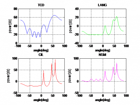
Table 1 shows the experiment setup of detection for Case-1. Figure 2 illustrates the resolution comparison for the algorithms TCD, LANG, CIL and NSM. For TCD algorithm unable to detect the sources, LANG, CIL and NSM are able to detect the sources at directions 10, 45 and 60 degree.
Table 1. Detection experiment setup for Case-1
|
Experimental Parameter |
Value |
|
Number of Array Elements |
8 |
|
Distance of Separation |
λ/2 |
|
Type |
Linear array |
|
Number of Sources |
3 |
|
Actual Direction of Sources |
[10 45 60] degree |
Table 2 depicts the Bias Comparison for Case-1 and Table 3 shows the time comparison with CIL having the lowest time followed by NSM, LANG and TCD.
Figure 2. Resolution comparison Case-1
Table 2. Bias comparison for Case-1
|
Algorithm |
Computed Bias |
|
TCD |
3.3228 |
|
LANG |
0.4580 |
|
CIL |
0.2286 |
|
NSM |
0.0258 |
Table 3. Time comparison for Case-1
|
Algorithm |
Time Taken (ms) |
|
TCD |
0.7411 |
|
LANG |
0.7400 |
|
CIL |
0.7369 |
|
NSM |
0.7386 |
Table 4. Detection experiment setup for Case-2
|
Experimental Parameter |
Value |
|
Number of Array Elements |
8 |
|
Distance of Separation |
λ/2 |
|
Type |
Linear array |
|
Number of Sources |
3 |
|
Actual Direction of Sources |
[10 15 20] degree |
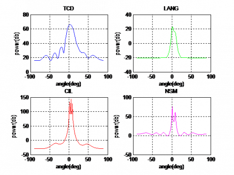
Figure 3. Resolution comparison Case-2
Table 4 represents the experiment setup for Case-2 and Figure 3 shows the shows the resolution comparison for Case-2. TCD and LANG are able to detect a single direction as compared to CIL and NSM. CIL and NSM algorithms are having higher resolution with the methods capable of detecting three directions.
Table 5. Bias comparison for Case-2
|
Algorithm |
Computed Bias |
|
TCD |
3.3228 |
|
LANG |
0.4580 |
|
CIL |
0.2286 |
|
NSM |
0.0258 |
Table 5 shows the bias comparison. As shown in the Figure 3. NSM has the lowest bias followed by CIL, TCD and LANG for low array elements and closely spaced directions.
Table 6. Time comparison for Case-2
|
Algorithm |
Time Taken (ms) |
|
TCD |
0.7411 |
|
LANG |
0.7400 |
|
CIL |
0.7369 |
|
NSM |
0.7386 |
Table 6 shows the time comparison with CIL having the lowest time followed by NSM, LANG and TCD and Table 7 defines the experiment setup of detection for Case-3.
Bias is the difference between the Estimated Direction and the Actual Direction, it provides the information about the system on how efficiently and effectively the Smart Antenna System is able to detect the user in the spatial domain.
Table 7. Detection experiment setup for Case-3
|
Experimental Parameter |
Value |
|
Number of Array Elements |
100 |
|
Distance of Separation |
λ/2 |
|
Type |
Linear array |
|
Number of Sources |
3 |
|
Actual Direction of Sources |
[10 45 60] degree |
Figure 4. Resolution comparison Case-3
Table 8. Bias comparison for Case-3
|
Algorithm |
Computed Bias |
|
TCD |
0.1149 |
|
LANG |
0.1149 |
|
CIL |
0.3539 |
|
NSM |
0.1170 |
For an efficient Detection Scheme the Bias values should to be very less, this is seen from the Table 8 which shows the bias comparison between different DoA Algorithms. The Figure 4 shows the different bias values that were computed TCD 0.1149, LANG 0.1149 and NSM 0.1170 had the lowest bias values followed by CIL 0.3539 which had the highest bias value amongst these algorithms. Noise Subspace Method (NSM) Algorithm provides consistent performance for Time complexity, High Resolution and maintains an Optimal Bias Level.
Table 9. Time comparison for Case-3
|
Algorithm |
Time Taken (ms) |
|
TCD |
0.8180 |
|
LANG |
0.8350 |
|
CIL |
0.9426 |
|
NSM |
0.8134 |
Noise Subspace Method (NSM) Algorithm generates the Subspace vectors, which enables the system to perform more complex signal processing techniques to achieve quick detection rate which takes less time duration and provides Optimal Bias values with High Resolution Detection. The Table 9 shows the Time complexity comparison (ms) between different DoA Algorithms, NSM 0.8134 took the shortest time duration to detect the user followed by TCD 0.8180, LANG 0.8350 and CIL 0.9426.
Table 10. Detection experiment setup for Case-4
|
Experimental Parameter |
Value |
|
Number of Array Elements |
100 |
|
Distance of Separation |
λ/2 |
|
Type |
Linear array |
|
Number of Sources |
3 |
|
Actual Direction of Sources |
[10 15 20] degree |
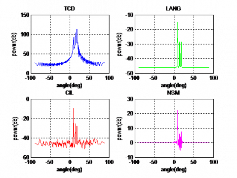
Figure 5. Resolution comparison Case-4
Table 10 shows the experimental set up for the case in which large antenna elements are used for detecting sources which are closely spaced.
The Figure 5 shows the resolution comparison. All four algorithms are capable of detecting the directions of sources. TCD, LANG, CIL and NSM are able to detect directions of 10, 15, 20 degrees.
Table 11. Bias comparison for Case-4
|
Algorithm |
Computed Bias |
|
TCD |
0.2839 |
|
LANG |
8.8783 |
|
CIL |
5.2008 |
|
NSM |
0.2286 |
Table 11 shows the bias comparison. As shown in the Figure 5, TCD has lowest bias as compared to other algorithms.
Table 12. Time comparison for Case-4
|
Algorithm |
Time Taken (ms) |
|
TCD |
0.7975 |
|
LANG |
0.8034 |
|
CIL |
0.9403 |
|
NSM |
0.8253 |
Table 12 shows the time comparison with TCD having lower time taken followed by LANG, then NSM and last is CIL.
Table 13. Beamforming experiment setup for Case-1
|
Experimental Parameter |
Value |
|
Number of Array Elements |
8 |
|
Number of Directional Element |
45 degree |
|
Number of Interference Elements |
3 |
|
Interference Directions |
[5 10 15] degree |
Table 13 is the input configured for the experiment with less number of array elements.
Figure 6. MSE comparison with lesser antenna array elements Case-1
The Figure 6 shows the MSE comparison. As shown in the Figure 7, LCWLCG has the lowest MSE as compared to WLM and WLCGM. The LCWLCG is getting converged at 45 iterations, WLM and WLCGM are getting converged at around 80 iterations.
Figure 7. Beamforming for Case-1
Table 14. Beamforming experiment setup for Case-2
|
Experimental Parameter |
Value |
|
Number of Array Elements |
100 |
|
Number of Directional Element |
45 degree |
|
Number of Interference Elements |
3 |
|
Interference Directions |
[5 10 15] degree |
For Case-2: Larger number of antenna array elements are used at the base station, the direction of the source is 45 degree with interference directions of 5, 10 and 15 degree, as shown in Table 14.
Figure 8. MSE comparison with larger antenna array elements Case-2
Figure 8 shows the MSE comparison for large number of antenna array elements that are used at the base station (BS). LCWLCG has the lowest error followed by WLCGM and WLM with LCWLCG converging at 25 iterations. 25 full Iterations are required to obtain the complete convergence of the signal, at the 24th iteration the signal has already entered into the convergence zone.
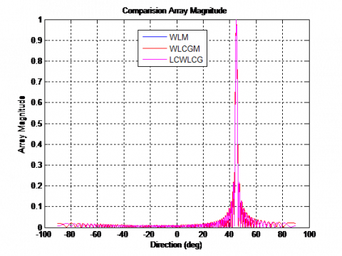
The Figure 9 shows the Beamforming when large number of antenna array elements are used at the base station a sharp narrow beam is produced towards the desired user present at 45 degree and spectral nulls towards the other interfering directions, this highly focused beamforming can be used for better data transmissions with less noise and interference in its way.
Figure 9. Beamforming for Case-2
In this paper performance analysis of algorithms for Direction of Arrival (DoA) methods as well as the Beamforming (BF) methods have been performed.
Experimental simulations are conducted and comparison is done for multiple cases with respect to the Bias, Resolution and Time complexity of each algorithm for the Direction of Arrival (DoA) methods, NSM DoA algorithm consistently delivered the following Bias [0.0258, 0.0258, 0.1170, 0.2286] and Time (ms) [0.7386, 0.7386, 0.8134, 0.8253], thus it is better for both the scenarios which uses smaller as well as larger number of antenna array elements.
Similarly for the case of Beamforming (BF) methods the Mean Square Error and Beam-directions have been computed and compared. The following comparison results were found: The MSE when working with fewer number of antenna array elements, the Low Complexity-Widely Linear Conjugate Gradient Method (LCWLCG) Algorithm provided the fast convergence rate of 45 iterations, whereas Weighted Linear Method (WLM) and Widely Linear Conjugate Gradient Method (WLCGM) got converged at 80 iterations.
When the large number of antenna array elements are used at the base station, the Mean Square Error (MSE) gets reduced and fast convergence rate of 25 Iterations is obtained by using the Low Complexity-Widely Linear Conjugate Gradient Method (LCWLCG) Algorithm. When LCWLCG Algorithm is compared with other algorithms such as Weighted Linear Method (WLM) and Widely Linear Conjugate Gradient Method (WLCGM) the signal convergence rate is very slow it almost takes around 80 iterations to get converged thus has higher mean square error value.
Beamforming using Smart Antenna System produces narrow sharp pencil-line main beam towards the desired user and deep spectral nulls are pointed towards other interfering users who are present at different angular directions in the spatial field, thus suppressing these unwanted interfering users improves the overall system throughput and efficiency.
The work reported in this research paper is supported by the college through the TECHNICAL EDUCATION QUALITY IMPROVEMENT PROGRAMME (TEQIP-III) of the MHRD, Government of India.
[1] Balanis, C.A. (2015). Antenna Theory: Analysis and Design. John Wiley & Sons.
[2] Prince, T.J., Elmansouri, M.A., Filipovic, D.S. (2021). A framework for design of multibeam antenna systems used for amplitude-only direction finding based on correlation method. In 2021 IEEE-APS Topical Conference on Antennas and Propagation in Wireless Communications (APWC), pp. 109-109. https://doi.org/10.1109/APWC52648.2021.9539529
[3] Liu, A., Shi, S., Wang, X. (2021). Efficient DOA estimation method with ambient noise elimination for array of underwater acoustic vector sensors. In 2021 IEEE/CIC International Conference on Communications in China (ICCC Workshops), pp. 250-255. https://doi.org/10.1109/ICCCWorkshops52231.2021.9538869
[4] Bassett, R., Foster, J., Gemba, K.L., Leary, P., Smith, K. B. (2021). The maximal eigengap estimator for acoustic vector-sensor processing. In 2021 Sensor Signal Processing for Defence Conference (SSPD), pp. 1-5. https://doi.org/10.1109/SSPD51364.2021.9541420
[5] Zhang, Q., Li, J., Li, Y., Li, P. (2021). A DOA tracking method based on offset compensation using nested array. IEEE Transactions on Circuits and Systems II: Express Briefs. https://doi.org/10.1109/TCSII.2021.3114025
[6] Lu, D., Duan, R., Yang, K. (2021). Closed-form hybrid Cramer-Rao bound for DOA estimation by an acoustic vector sensor under orientation deviation. IEEE Signal Processing Letters, 28: 2033-2037. https://doi.org/10.1109/LSP.2021.3114125
[7] Zheng, Z., Huang, Y., Wang, W.Q., So, H.C. (2021). Augmented covariance matrix reconstruction for DOA estimation using difference coarray. IEEE Transactions on Signal Processing, 69: 5345-5358. https://doi.org/10.1109/TSP.2021.3113468
[8] Mao, Y., Guo, Q., Ding, J., Liu, F., Yu, Y. (2021). Marginal likelihood maximization based fast array manifold matrix learning for direction of arrival estimation. IEEE Transactions on Signal Processing, 69: 5512-5522. https://doi.org/10.1109/TSP.2021.3112922
[9] Wang, S., Nie, K., He, M., He, Y. (2021). DOA estimation aided by magnitude measurements. IEEE Transactions on Vehicular Technology, 70(11): 12197-12202. https://doi.org/10.1109/TVT.2021.3113136
[10] Liu, Y., Yan, Y., You, L., Wang, W., Duan, H. (2021). Spatial covariance matrix reconstruction for DOA estimation in hybrid massive MIMO systems with multiple radio frequency chains. IEEE Transactions on Vehicular Technology, 70(11): 12185-12190. https://doi.org/10.1109/TVT.2021.3113018
[11] Xu, X., Shen, M., Zhang, S., Wu, D., Zhu, D. (2021). Off-grid DOA estimation of coherent signals using weighted sparse Bayesian inference. In 2021 IEEE 16th Conference on Industrial Electronics and Applications (ICIEA), pp. 1147-1150. https://doi.org/10.1109/ICIEA51954.2021.9516237
[12] Li, J., Zhao, J., Ding, Y., Li, Y., Chen, F. (2021). An improved co-prime parallel array with conjugate augmentation for 2-D DOA estimation. IEEE Sensors Journal, 21(20): 23400-23411. https://doi.org/10.1109/JSEN.2021.3106382
[13] Yin, B., Liu, Q. (2021). Direction-of-arrival estimation using joint sparse reconstruction based on acoustic vector array. In 2021 OES China Ocean Acoustics (COA), pp. 811-815. https://doi.org/10.1109/COA50123.2021.9519943
[14] Zhou, W., Wang, Z., Xie, Z. (2021). High-resolution DOA estimation algorithm of vector hydrophone based on preselected filter. In 2021 OES China Ocean Acoustics (COA), pp. 946-949. https://doi.org/10.1109/COA50123.2021.9520068
[15] Salama, A.A., Morsy, M.E., Darwish, S.H. (2021). A novel low complexity CS-based DOA estimation technique. In 2021 International Telecommunications Conference (ITC-Egypt), pp. 1-4. https://doi.org/10.1109/ITC-gypt52936.2021.9513925
[16] Yadav, S.K., George, N.V. (2021). Coarray MUSIC-group delay: High-resolution source localization using non-uniform arrays. IEEE Transactions on Vehicular Technology, 70(9): 9597-9601. https://doi.org/10.1109/TVT.2021.3101254
[17] Li, X.W., Wang, J.H., Li, Z., Li, Y.J. Chen, M., Zhang, Z. (2021). Leaky-wave antenna array with bilateral beamforming radiation pattern and capability of flexible beam switching. IEEE Transactions on Antennas and Propagation, 70(2): 1535-1540. https://doi.org/10.1109/TAP.2021.3111157
[18] Belay, H., Kornegay, K., Ceesay, E. (2021). Energy efficiency analysis of RLS-MUSIC based smart antenna system for 5G network. In 2021 55th Annual Conference on Information Sciences and Systems (CISS), pp. 1-5. https://doi.org/10.1109/CISS50987.2021.9400325
[19] Kim, J., Lee, H., Park, S.H. (2021). Learning robust beamforming for MISO downlink systems. IEEE Communications Letters, 25(6): 1916-1920. https://doi.org/10.1109/LCOMM.2021.3063707
[20] Da Silva, J.M.B., Ghauch, H., Fodor, G., Skoglund, M., Fischione, C. (2021). Smart antenna assignment is essential in full-duplex communications. IEEE Transactions on Communications, 69(5): 3450-3466. https://doi.org/10.1109/TCOMM.2021.3059463
[21] Qian, X., Di Renzo, M., Liu, J., Kammoun, A., Alouini, M.S. (2020). Beamforming through reconfigurable intelligent surfaces in single-user MIMO systems: SNR distribution and scaling laws in the presence of channel fading and phase noise. IEEE Wireless Communications Letters, 10(1): 77-81. https://doi.org/10.1109/LWC.2020.3021058
[22] Mei, W., Zhang, R. (2020). Cooperative beam routing for multi-IRS aided communication. IEEE Wireless Communications Letters, 10(2): 426-430. https://doi.org/10.1109/LWC.2020.3034370
[23] Komeylian, S. (2020). Performance analysis and evaluation of implementing the MVDR beamformer for the circular antenna array. In 2020 IEEE Radar Conference (RadarConf20), 1-6. https://doi.org/10.1109/RadarConf2043947.2020.9266505
[24] Krishnamoorthi, S., Macwan, A., Oh, P., Kwon, S.S.C. (2020). Interference-aware multi-user, multi-polarization superposition beamforming (MPS-beamforming). In 2020 IEEE Green Energy and Smart Systems Conference (IGESSC), pp. 1-6. https://doi.org/10.1109/IGESSC50231.2020.9284988
[25] De Cordova, P.P.F., Orozco-Tupacyupanqui, W. (2020). Comprehensive intelligent optimization of an N-element uniform linear array using genetic algorithms and adaptive filtering. In 2020 IEEE ANDESCON, pp. 1-6. https://doi.org/10.1109/ANDESCON50619.2020.9272086
[26] Reza, M.F., Hossain, M.S., Rashid, M.M. (2020). Performance study of NVL technique based robust uniform concentric circular array beamformer under mismatch condition. In 2020 IEEE Region 10 Symposium (TENSYMP), pp. 953-956. https://doi.org/10.1109/TENSYMP50017.2020.9230711
[27] Sasi, A., Jaya, J. (2020). Multilevel optimized beam forming technique for 5G. In 2020 6th International Conference on Advanced Computing and Communication Systems (ICACCS), pp. 957-960. https://doi.org/10.1109/ICACCS48705.2020.9074419
[28] Zheng, Z., Yang, T., Jiang, D., Wang, W.Q. (2019). Robust and efficient adaptive beamforming using nested subarray principles. IEEE Access, 8: 4076-4085. https://doi.org/10.1109/ACCESS.2019.2963356
[29] Gaydos, D., Nayeri, P., Haupt, R. (2019). Adaptive beamforming in high-interference environments using a software-defined radio array. In 2019 IEEE International Symposium on Antennas and Propagation and USNC-URSI Radio Science Meeting, pp. 1501-1502. https://doi.org/10.1109/APUSNCURSINRSM.2019.8888670
[30] Choi, J. (2011). Opportunistic beamforming with single beamforming matrix for virtual antenna arrays. IEEE Transactions on Vehicular Technology, 60(3): 872-881. https://doi.org/10.1109/TVT.2011.2113197
[31] Mishra, D., Johansson, H. (2019). Optimal channel estimation for hybrid energy beamforming under phase shifter impairments. IEEE Transactions on Communications, 67(6): 4309-4325. https://doi.org/10.1109/TCOMM.2019.2901790