Muhammad Shoaib* | Nasir Sayed
© 2022 IIETA. This article is published by IIETA and is licensed under the CC BY 4.0 license (http://creativecommons.org/licenses/by/4.0/).
OPEN ACCESS
For a range of medical analysis applications, the localization of brain tumors and brain tumor segmentation from magnetic resonance imaging (MRI) are challenging yet critical jobs. Many recent studies have included four modalities: i.e., T1, T1c, T2 & FLAIR, it is because every tumor causing area can be detailed examined by each of these brain imaging modalities. Although the BRATS 2018 datasets give impressive segmentation results, the results are still more complex and need more testing and more training. That’s why this paper recommends operated pre-processing strategies on a small part of an image except for a full image because that’s how an effective and flexible segmented system of brain tumor can be created. In the first phase, an ensemble classification model is developed using different classifiers such as decision tree, SVM, KNN etc. to classify an image into the tumor and non-tumor class by using the strategy of using a small section can completely solve the over-fitting problems and reduces the processing time in a model of YOLO object detector using inceptionv3 CNN features. The second stage is to recommend an efficient and basic Cascade CNN (C-ConvNet/C-CNN), as we deal with a tiny segment of the brain image in each and every slice. In two independent ways, the Cascade-Convolutional Neutral Network model extracts learnable features. On the dataset of BRATS 2018, BRATS 2019 and BRATS 2020, the extensive experimental task has been carried out on the proposed tumor localization framework. The IoU score achieved of three datasets are 97%, 98% and 100%. Other qualitative evaluations & quantitative evaluations are discussed and presented in the manuscript in detail.
brain tumor, magnetic resonance imaging, YOLO detector, inception-V3, segmentation
The most common brain tumor is glioma, which also has the highest rates of mortality and highest rates of morbidity. For the diagnosis and curing of glioma, the accuracy of segmentation is very critical. The treatment and diagnosis of brain tumor can be caused by using the necessary tool known as magnetic resonance imaging (MRI) [1]. Various MRI sequences can present various tissue structures of brain tumor, and multimodal MRI of brain tumors is usually used to segment brain tumors. As there is a complex structure of brain tumor, individual differences and uncertainty in the boundaries of the tumor, the segmentation of the brain is not an easy task to do [2]. A lot of time is required by doctors in order to complete the manual segmentation, and the accuracy of the segmentation is poor. During the last years, deep learning-based automatic segmentation methods have demonstrated promising results in the segmentation of medical imaging [3]. The classification, object detection, and segmentation are computer vision tasks; these tasks by the deep learning process, if based on CNN, will perform much better. A CNN can learn complex data features without depending on manual feature extractions during the training process, improving brain tumor segmentation accuracy [4, 5].
A fully convolutional neural network (FCN) was proposed by Long et al. [6], which used the upsampling for restoring the map of the output to the same size as the image input and achieved semantical end-to-end image segmentation by converting the full connection layer into convolutionary layer. A U-net technique is proposed by Ronneberger et al. [7] to segment biological cells, consisting of two paths, i.e. contraction and expansion.
A contraction path includes max pooling used for down-sampling and convolution block used for the extraction of features. An expanding path includes the up-sampling instead of the down-sampling and a convolution block. If the connection is skipped between these two paths (i.e. contracting path & expanding path), then the features of exact resolution will be fused. U-net consists of simple structures and can achieve better segmentation results in medical images with a small sample size. Contrary to this, image segmentation of brain tumors based on U-net applications should be improved [8]. The U-contracting net's path, on the other hand, employs the shrinking of feature map by pooling layer and thus, cause the expansion of the receptive field.
Continuous pooling can result in providing no details of the image and have an impact on segmentation results. On the other hand, the essential problems are the differences in the size, shape, and location of brain tumors, as well as in obtaining more detailed segmentation target features and multiscale features [9]. The residual network [10] was proposed for solving the problems of gradient disappearance and network degradation as network depth increases. The addition of identity mapping b/w the input & the output of numerous convolutional layers makes the network converge easier and prevents network degradation [11].
A DeepLab model is proposed by Chen et al. [12], which is used to obtain multiscale features. The final pooling layer was removed in this model, and atrous convolutions expanded the receptive field. The input is sampled in parallel position by atrous spatial pyramid pooling (ASPP) with atrous convolutions of many different dilation rates; then, the results are spliced together. The extraction of multiscale features is better with ASPP. An inception network was proposed by Szegedy et al. [13]. The network's width can be increased by using the inception module. In the ILSVRC 2014 competition, GoogLeNet, which included the inception module, had outstanding classification results and detection results. To reduce image data loss, this paper proposes extending the receptive field by utilizing atrocious convolution and decreasing pooling layers. An atrous convolution is a process that involves the insertion of holes in a standard convolution kernel for expanding the feature extraction’s receptive field with no additional parameters [14].
We discovered some issues in the automatic segmentation of brain tumors by looking through the literature: (a) Highly Imbalanced Tumor over Background, (b) Inconsistency in Appearance, and (c) Similarity between tumor and healthy tissue. The difficulty in segmenting brain tumors is primarily due to the wide range of sizes, shapes, regularity, location, and appearance of brain tumors. Segmenting tumors from background is a highly imbalanced dense prediction task because the tumor area only accounts for a small portion of the whole slice image in some benchmark datasets, usually less than 1%. When using a machine learning model to perform automatic segmentation, it's important to keep such issues in mind. Even if they belong to the same connected component, different parts of a tumor can have different appearances. The appearance of different slices of brain tumors is usually quite different. The difficulty of methods based on appearance models is exacerbated by the fact that some tumors have inconsistent appearances. Also, when using machine learning techniques, the features extracted should account for this type of variation in appearance. Surrounding healthy tissues can sometimes resemble tumors. The tumor and the background have a similar appearance in this case. Even if strong contrast boundaries exist between the tumor and healthy tissue, the intensity contrast information can still be used to segment the tumor. Otherwise, it is difficult for an untrained human to locate a tumor. A tumor can look a lot like other parts of the brain in many cases. This type of tissue can make the segmentation process even more difficult. It will be difficult to distinguish tumor from background and correctly predict labels using a machine learning model.
This paper represents the combination of inception and atrous convolution to form the A-Inception module, and new U-net-based network architecture is proposed. To increase the network’s depth & width and then obtain different sizes of the receptive field, the encoder of the network uses a module of A-inception. At the same time, the network is enhanced with atrous spatial pyramid pooling for extracting the image's multiscale features.
The proposed brain tumor segmentation model is trained on three benchmark datasets. The performance achieved by the best model is (a) mean Dice score: Enh = 0.923, Whole 0.931, Core = 0.886, (b) mean sensitivity score: Enh = 0.937, Whole 0.943, Core = 0.982, and (c) HAUSDORFF99: Enh = 1.76, Whole 1.57, Core = 2.48.
Section 2 consists of a detailed literature review and its summary; section 3 is the research methodology section in which the framework of the proposed model is discussed along with the mechanism of extracting learnable features and Yolo version 3 architecture for tumor segmentation, the section 4 contains information about the experimentation performed, performance evaluation and comparison of segmentation results with state-of-the-art. The article finishes with Section 5, which serves as a summary of the article and future directions of the research.
In the computer vision field, approaches that rely on convolutional neural networks have done well in recent years. In contrast to traditional methods, convolutional neural network algorithms may learn the complicated features of actual data and do not depend on the extraction of annual features that improve image segmentation accuracy [15]. In the segmentation of an image, the encoder-decoder structure is prevalent. The image pixels are mapped in a higher-dimensional distribution during the encoding approach, and the process of decoding gradually recovers the image's detailed information and spatial dimensions. As a result, the encoder-decoder structure can achieve comprehensive image semantic segmentation [16]. SegNet [17] in image segmentation is typically a framework of encoder-decoder. SegNet's encoder community contains the same type of topology as VGG16's convolution layer, without the completely connected layers. The max-pooling is a technique used for reducing the dimensions of feature mappings—the decoder used nonlinear upsampling in its input map by using max-pooling indices received by the equivalent encoder. The U-net is a type of encoder-decoder that was used extensively in the segmentation of the medical image. It introduces skip connections b/w the encoder and the decoder that can combine the feature map with the encoder and decoder's exact resolution. Attention gates were introduced by Oktay et al. [18] to the conventional U-internet architecture, which regularly focuses on the targeted structures of all shapes & sizes. By introducing a dense connection and replacing the basic convolution module with a dense connection module in U-internet, Shaikh et al. [19] improved the network's segmentation performance. At some point during the training process, the attention weight of the target region progressively shifted to the target region. In contrast, the attention weight of the targeted region progressively declined, improving the accuracy of segmentation.
CNN employs pooling for achieving down-sampling that reduces image length while increasing the receptive field. Then for restoring the original image length, up-sampling is done within the semantic segmentation of images. Some image details may be lost as a result of this procedure [20]. You may raise the receptive field, and it does not sacrifice image resolution with atrous convolution, which improves picture semantic segmentation accuracy. Zhao et al. [21] developed a pyramid scene parsing network (PSPNET) that improves the network's ability to gather global records by combining the context of different locations using a pyramid pooling module.
DeepLabv3 [22] proposes connecting multiple atrous convolutions, including different rates of dilation in series & parallel to segment’s multiscale objects, resulting in large receptive fields of cascade mode & diff. Receptive fields for the same input in the parallel mode, allowing for more multiscale feature extraction.
DenseASPP [23] uses dense connections to integrate atrous convolution with diff. Rates of dilation. The field of receptive of output neurons is expanded without a pooling operation, leading to output features that cover a wide range of semantic information and acquire multiscale features. ASPP is a fully spatial pyramid pooling-based development. DeepLabv3+ [24] is a DeepLabv3 version with a simple decoder module for better details of object boundary. For the segmentation of multiscale objects, parallel pooling modules are used to extract multiscale features.
Automated brain tumor segmentation has sparked a lot of interest in the scientific community, and it's still being researched. Maximum medical image researchers utilized traditional standard image processing techniques before 2010, threshold value based grouping of pixel [25] and seed point selection based region growing segmentation [26]. Suzuki and Toriwaki performed ROI (lesion) segmentation using an adaptive threshold segmentation [25], but optimal threshold value selection for image with reduced contrast is a serious issue for the proposed technique. Region growth was proven to be an effective brain tumor segmentation method in 2005. The amount of computation is less when compared to other non-region-based methods, especially for homogeneous tissues and regions [26]. Achieving higher accuracy on segmenting medical images never touch the radiologist expectation, even though they are simple to implement and require little computation. As a result, it is primarily used for two-dimensional segmentation [27]. Artificial Intelligence particularly machine learning technology [28] has gradually been implemented to analyse biomedical images since the 2005. Segmentation of brain lesions have also been performed using various supervised learning (classification) and unsupervised learning (clustering) approaches [29-31]. Fletcher-Heath et al. applied Fuzzy C Means cluster to group the MRI pixel, the pixel belonging to the tumor region are all grouped to the same cluster and using image processing techniques the segmentation image is further process to detect the entire tumor with greater accuracy [29]. Zhou et al. developed a novel framework for MRI images based tumor segmentation using support vector classifier [30]. Based on multi-window Gabor high pass filters and an adapted technique develop through Markov Random Field, Subbanna et al. developed a probabilistic brain and tumor automatic segmentation model [31]. These methods can improve accuracy when compared to traditional segmentation methods. In clinical practice, however, more accurate methods are still required. Deep learning methods have progressed over the last ten years as computing power has increased dramatically. Instead of using pre-defined manual features, deep neural networks can learn hierarchical features from input images. Convolutional Neural Networks and Recurrent Neural Networks are two of the most popular deep learnings approached that has been extensively used for the segmentation and classification of medical images that ranges from X-ray mammogram images [32] to chest CT DICOM image for COVID-19 analysis [33]. The same CNN deep learning approached are also used by several medical image analyst for tumor segmentation. which has piqued researchers' interest.
In 2014, Zikic et al. found that CNNs were more accurate than traditional machine learning methods for brain tumor segmentation [34]. Brosch et al. used a deep 3D convolutional encoder network with two interconnected routes: convolution and deconvolution, to perform segmentation in 2016. Each image has a different pattern and for training the network very less data was required [35]. Multiple routes based neural network for brain tumor segmentation was proposed in 2017 [36], which was an augmented version the conventional feed forward neural network. In 2019 and 2020, Sharif and Amin et al. proposed several brain tumor segmentation algorithms [37, 38] to improve segmentation accuracy and speed up processing. Our proposed brain tumor segmentation model is based on the U-Net [7, 39] deep learnings model, the only difference is the augmentation process where all 2D based filtering and processing is replaced by 3D operations. The proposed brain tumor segmentation framework incorporates a multi-path network which is capable of performing segmentation with higher accuracy.
Despite significant progress in brain tumor segmentation, there are still a number of issues and challenges to be addressed. Gliomas are first and foremost glial cell mutations. Gliomas can appear anywhere in the brain due to the wide spatial distribution of glial cells. Furthermore, because the shape and size of brain tumors vary greatly between patients, there is little a priori information about tumor shape and size available prior to segmentation. The combination of positional and morphologic uncertainty makes accurate brain tumor localization difficult. Second, an MRI that can image in multiple directions can provide tissue detail. Because 3D imaging methods are better for detecting brain tumors, we primarily use MRI to segment them. However, MRI calculations during automation are complex, and image analysis usually takes longer. Platforms for segmentation processing must meet stringent performance requirements. Deep learning methods can achieve high accuracy rates in brain tumor segmentation tasks, it can be concluded. However, the process of segmenting brain tumors can take a long time and require a lot of computing power. As a result, for high-precision brain tumor detection and efficient acquisition of detection results, speeding up CNN-based 3D brain tumor segmentation is critical. GPUs are currently used to speed up the segmentation process for brain tumors, but the speed and power consumption could be improved. CNN uses two methods for brain tumor segmentation: training and inference. The process of training is an iterative process of adjusting training parameters. During the training process, the model's output is compared to the expected result, and the parameters are updated to minimise the difference. This process is repeated until the output converges to a value that closes the gap to a safe level. Training is typically an offline process that can be planned ahead of time. Our work focuses on accelerating the inference process because it is a real-time process.
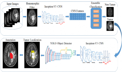
As shown in Figure 1, the proposed technique comprises four basic steps: (1) enhancement, (2) classification, (3) localization, and (4) segmentation. Homomorphic wavelet filers are used for enhancing the input images and inceptionv3 derived deep features are used for input image classification. The identified images are segmented using Kapur entropy and localised using the proposed YOLOv2-inceptionv3.
3.1 Noise elimination using homomorphic wavelet filter
The images obtained from an MRI procedure with adverse conditions may be affected by noise, lowering the disease detection rate. For noise reduction, there are several filters available. These filters are dependent on the sort of noise present in the photos. The images are represented in frequency domain using the wavelet transform. Image is divided into three bands via decomposition: high to high (i.e., HH), low to high (i.e., LH) & high to low (i.e., HL). This study looks into the homomorphic wavelet filter decomposition for removing speckle noise, which is described mathematically as follows:
$\log _{f(x, y)}=\log _{g(x, y)}+\log \eta_{m}(x, y)$ (1)
Figure 1 depicts the use of homomorphic filter for noise removing process and wavelet decomposition, with the image split into four bands: i.e., High-Low, Low-High, High-High, and Low to High-High to High. When compared to other bands like HL, LH & LH-HH, the HH bands improve the quality of image. As a result, the High-High band is used to accomplish accurate segmentation for further processing.
3.2 Extracted deep features using pre‑trained inceptionv3 architecture
The applications like deep learning, speech recognition and computer vision are commonly used in artificial intelligence applications. However, as the field of deep learning becomes more popular, categorization into corresponding categories has become a big issue. Because correct models & architecture are developed in the time-saving manners, this challenge might be handled through transfer learning. Instead, then learning new features from start, this method involves leveraging previously acquired patterns to address various challenges. For problem solving, transfer learning employs pre-trained models; these models have been learned over a large data.
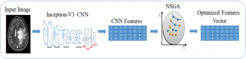
As a result, for feature learning, this study employs a pre-trained inceptionv3 transfer-learning model that includes 01 image, 094 batch-normalization (bn), 094 Convolutional, 14 max-pooling, 094 ReLU, softmax with the function of cross-entropy, 015 depth concatenation and fully connected layers. As shown in Figure 2, features are retrieved from completely connected layers termed prediction and then transferred to NSGA for improved feature selection.
In the first phase of our framework that is depicted in Figure 1, an ensemble supervised learning classification model is developed; using the bagging strategy, multiple classifiers are trained, and in the validation phase, a voting scheme is applied to the output achieved through several classifiers and predict whether the image is from the normal class or abnormal class containing single or multiple tumors. In the second phase, a Yolo-V3 based on inception-V3 CNN features is trained on tumor containing MRI image along with its annotated ground truth that has been provided by the radiologist, the ensemble classification method helps to only process the images that contain tumor without wasting time for detecting of tumor in normal images. In most Yolo architecture, Darknet CNN, which is 153 layers model, is used for features learning; in this framework, the Darknet model has been replaced with inception-V3 315 layers model to extract more robust features from images and improve the detection accuracy of the YOLO detector. In Table 1, the details of our proposed segmentation models are discussed as: in step 1, the homomorphic filter is applied to enhance the quality of medical images. Step 2 is the features extraction phase, where inception-V3 CNN architecture is used for feature learning from normal and tumors containing MRI images. In step 3, an ensemble classification model is used to detect tumor and non-tumor images. Finally, in step 4, the Inception-V3 features based YOLO object detector is used to localize and segment the brain tumor regions.
Figure 1. Our proposed brain tumor segmentation and classification models architectures
Figure 2. Learning based features extraction using inceptionv3 CNN model
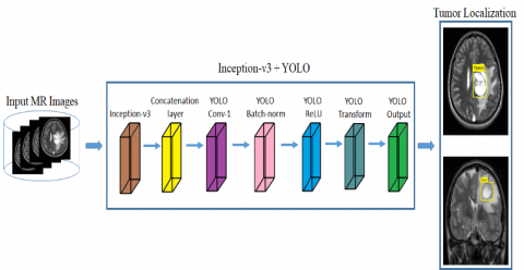
Figure 3. Localizing the tumor in MRI images using proposed model
Table 1. Proposed tumor segmentation framework details
|
Step No. |
Purpose |
Technique |
Output |
|
Step 1 |
Image Enhancement |
Homomorphic filtering
|
Enhance image |
|
Step 2 |
Features Extraction |
Inception-V3 CNN |
Feature Map |
|
Step 3 |
Ensemble Classification |
SVM, decision tree and KNN |
Classify into ‘Tumor’ or ‘Normal’ |
|
Step 4 |
Tumor Detection |
Inception-V3 Features + Yolo Object Detector |
Localization and Segmentation of Tumor |
3.3 Features selection
Using the inceptionv3 network, a deep feature vector (1 x 1000) is obtained. The engineering features are used to choose the best feature vector using NSGA II. As seen in Table 2, the NSGA parameters are as follows.
Table 2. The parameters about NSGA II
|
Maximum Number of Iterations |
200 |
|
Population size |
25 |
|
Crossover Percentage |
0.7 |
|
Number of offspring |
2 x round (crossover x 25/2) |
|
Proportion of mutation |
0.1 |
|
Mutation percentage |
0.4 |
|
Total Mutants No |
Mutation percentage x 25 |
3.4 Localization using YOLO‑inceptionv3 model
To locate the tumor location, a YOLO-inceptionv3 model is proposed which have 174 layers, with inceptionv3 having 165 layers with 01 input, 50 Conv, 50 bn, 50 activations ReLU, 06 mixed (depth concatenation), 03 max-pooling, 05 average pooling, and 09 layers of tinyYOLOv2 [40] model. Table 3 consists of several hyperparameters used to train our proposed tumor localization and segmentation framework. The model is also trained on some other hyperparameters as well, but the hyperparameters in the table listed are the most optimal through which the tumor is segmented with higher accuracy. As seen in Figure 3, the proposed model more precisely localises the tumor location. The MSE loss between predicted bounds and boxes of ground truth was optimised using the YOLOv2 model. Three main sorts of losses are used to train the model: localization, confidence, and classification. Localization loss computes error utilising location, estimating box size & ground truth among the expected and ground truth boxes. The objectiveness having error with detected objects in the jth limited box of grid I cell is computed using the confidence loss. The classification loss was used to compute probability for each grid cell class.
Table 3. Adjusts the hyper-parameters ofinceptionv3 CNN based YOLOv2 model
|
Epochs |
100 |
|
Mini Batch Size |
16 |
|
Initial Learning Rate |
0.1 |
|
Momentum |
0.7 |
|
Optimizer |
Adam |
Table 4. Details of the BRATS MRI images dataset
|
Dataset Year |
No. of Training Images |
No. of Testing Images |
|
2018 |
20515 |
20515 |
|
2019 |
21978 |
21978 |
|
2020 |
25692 |
25692 |
3.5 Lesion segmentation
Variability in medical data is a major difficulty in medical imaging. Different modalities, such as X-ray, MRI, CT, and PET, show variances in human anatomy. The illness severity levels are analysed using the segmentation region. McCulloch's Kapur entropy approach [41] is used to segment tumors in the proposed method. In this method, the foreground and background regions' likelihood of intensity values distributions are measured, and entropy is calculated independently for each region. To enhance the total of their entropies, the best threshold value is used. In Figure 4, four different images are visualized; Figure 4-a is the input of volumetric MRI series to the segmentation deep learning model, the Figure 4-b is the output of Kapur based entropy method for tumor localization. Figure 4-c is the segmented brain tumor (lesion) in multiple MRI slices, and Figure 4-d is the overlay images of the segmented tumor and original MRI images where the segmented and localized tumor can be seen in the red color.
3.6 Data and implementation details
The dataset of BRATS 2018 that comprises of brain tumor Multiview and multiseries MRI images along with ground-truth (segmented mask) by the domain experts, the brain tumor subjects have various histological subregions of heterogeneity, with a wide difference of aggressiveness & medical history. The MRI images of BRAT dataset is used for model training and model validation for performance analysis. These datasets Multi-Modal MR images details can be seen in the Figure 5, which are different from Computed Tomography (CT) images containing the dimensions of 240 240 150 and also were obtained clinically, utilising diverse strength of magnetic field, scanners, & varied protocols from several institutes. The MRI FLAIR series highlights the tumor region, whereas the cerebral spinal fluid, fat layer are not visible in this contrast level. The T2 weight series is consider to be the most appropriate and feasible for tumor analysis, the voxel contrast intensity of the tumor, cerebral spinal fluid and fat in the head region are almost the same, which makes it more challenging to detect and segment using an automatic diagnosis system. Other than FLAIR and T2 W MRI images, the T1 W and T1 Contrast series is also studied for tumor confirmation and treatment plans.
Figure 4. (a) Load Input Image (b) Kapur entropy-based image (c) segmentation of lesion (d) overlaying segmented tumor region over the original images
Figure 5. Overview of the benchmark BRATS dataset used for models validation
This dataset contains 75 LGG cases & 210 HGG cases that were divided randomly into the training data (i.e. 80%), validation data (ten percent), and test data (ten percent). In addition, neuroradiologists labelled images with tumor labels (necrosis is represented by 1, edema is represented by 2, non-enhancing tumor is represented by 3, and enhancing tumor is represented by 4). Also, a tissue with a value of zero is considered normal). The third label isn't used.
The proposed structure's experimental results were obtained using MATLAB 2020b on an Intel Core I7 9th generation CPU, with a 48 GB of RAM and a total of 15 L3 cache. To speed up the training processing by incorporating parallel computing CUDA framework was used with RTX 2070 super 8 GB NVIDIA GPU, the MATLAB was running on windows 10 64-bit operating system. For the training stage, we used Adaptive Moment Estimation (Adam) with 2 batch sizes, 10-5 weight decay and an initial rate of learning of 10-4. We spent a total of 13 hours training and 7 seconds testing each volume.
3.7 Evaluation measure
Metrics for the enhancing core, tumor core (TC, which includes necrotic core & non-enhancing core), and total tumor are used to evaluate the approach's success (WT, which includes all the classes/types of tumor structures). In case of image segmentation, the Dice Similarity Co-efficient (DSC) is used as an evaluation metric that help to compute the number of overlapped pixel between the actual pixel (ground-truth) and the pixel predicted by the model. Three criteria were used to generate the experimental results: HAUSDORFF99, the Dice similarity, and models achieved Sensitivity. Hausdorff score is a measure to calculate the distance b/w a predicted region and ground-truth region. The overlap between the ground truths and the predictions is computed using a dice score as the evaluation metric. The measure of correctly determined non-tumor pixels is called specificity (real negative rate). Sensitivity refers to the number of tumor pixels that were estimated accurately. These 3 criteria are as follows:
$\operatorname{DICE}\left(R_{p}, R_{a}\right)=2 * \frac{R_{p} \cap R_{a}}{R_{p}+R_{a}}$ (2)
Sensitivity $=\frac{\left(R_{p} \cap R_{a}\right)}{R_{a}}$ (3)
where, Rp demonstrated the predicted tumor regions, Ra demonstrated the actual labels and Rn demonstrated the actual non-tumor labels.
To gain a better understanding of the tumor segmentation performance and to make quantitative and qualitative comparisons, we used five different models (Multiple models Cascaded [42], Cascading of random forests classifier [43], Cross MRI imaging modality [44], Task Structure [45], and One-Pass Multi-Task [46]). Table 5 shows quantitative results for several types of segmentation algorithms proposed.
Table 5 shows that without applying a pre-processing technique, the two-route CNN model is unable to partition the tumor area effectively. When a mechanism of attention is added neural network model with multiple paths without employing some pre-processing or enhancement method, the segmentation results improve in all three criteria. Dice scores in three tumor locations increased from 0.2532, 0.2797 for Enh, 0.2143 to 0.8756 for core, and from 0.8551 to 0.8716 for Whole, after adopting the pre-processing strategy. Despite just having a single-route Convolutional Neutral Network model (global features or local features), the Convolutional Neutral Network model consistently improves the performance of segmentation in all tumor regions because to the pre-processing strategy. Furthermore, it has been discovered that applying the pre-processing method has a greater impact than simply by the use of attention mechanism. It can also be stated as that when we deal with only a small portion of an input image that has been recovered by pre-processing method, the attention mechanism which was proposed would be more useful. When the effects of local and global features are compared, it is clear that local features outperform global features.
Table 6 lists the HAUSDORFF99 values, Dice values and sensitivity values for all of the input images by using all structures. The greatest Dice values, Sensitivity values, and the smallest values of HAUSDORFF99 are indicated in bold for each index in Table 6. Table 6 shows that our technique achieves the maximum Sensitivity values in the Enh & Whole tumor areas, with the Core area of highest value being 10.
There is also a minimal variation between the HAUSDORFF99 values when the researches [46, 47] are used.
For all three criteria, there are significant improvements in Enh area [44]. Also, on the HAUSDORFF99 measure, had the worst outcomes in the Whole and Core areas [45]. Not only were all criteria improved when utilising the proposed method compared to the previous approaches discussed, but the value of sensitivity in Core area using [47] is still greater. There are three explanations, as far as we know. First, before applying the four modalities to the CNN model, the proposed technique pays special attention to deleting inconsequential regions within them. Second, our method investigates the richer context tumor segmentation by combining local information and global information with varying numbers of convolutional layers. Third, the network can be biassed to an appropriate output class by taking into account the influence of the dissimilarity between the tumor's centre and the projected area. Furthermore, by simply using a simple CNN structure, our approach achieves very promising performances and reduces running time when compared to state-of-the-art algorithms using heavier networks, such as [45, 46]. Furthermore, as shown in Table 8, the proposed approach is faster than other evaluated models at segmenting the tumor.
In Table 7, the tumor segmentation time of various detection models is listed. The time for 50 images segmentation has been calculated in seconds, and then by taking the mean of the 50 images times, the average segmentation time of each model is calculated. The above table shows that using the YOLO model on MRI images for tumor segmentation enhances detection and localization efficiency by outperforming other state-of-the-art methods.
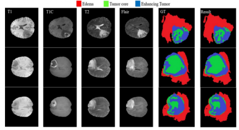
In Figure 6, three brain tumor cases are visualized where each of the tumor cases consists of T1W, T1C, T2W, FLAIR and ground truth images which are annotated by the domain expert manually. The final images in Figure 6 are the segmented results of three cases; the red region in the lesion indicates the edema region, the green region represents the tumor core area, and the blue region is the enhanced tumor segmentation results. Every region has a common border with every other region, as illustrated. The border between tumor core & enhancing area inside the T1C pictures (3rd column) may be easily differentiated with high accuracy rate with no use of other modalities because of the difference in value of enhancing areas & tumor core. When dealing with the border of a tumor core, edoema areas, or exacerbated edoema areas, however, this is not the case. Because of the aforementioned properties of each modality, we see that reducing the searching area eliminates the requirement for a highly deep CNN model.
Our model's DWA module can collect more related tumor and brain information, resulting in better segmentation results. As illustrated in Figure 7, the addition of the DWA module to the proposed techniques enhances segmentation, especially at the edge of tumor containing areas.
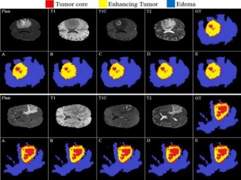
In Figure 8, the comparison of the baseline and our model demonstrates the efficiency of the proposed method in distinguishing between all four zones. Figure 8 shows the ground reality for all four modalities (GT). Although the Edema region are detected by the well performance of multi-cascade (Figure 8-A) and cascading random forests techniques (Figure 8-B), but minor Edema patches cannot be detected by them, outside of the main Edema body. The Cross-modality (Figure 8-C) and One-Pass Multi-Task (Figure 8-D) techniques show promise in detecting tumor Core and Enhancing areas, particularly tumor Core at the Enhancing area's outside border. The Crossmodality approach is used to show how some separated Edema zones get stuck together between the final segmentation. Applying the Cross-modality structure, as illustrated in Figure 8(C), achieves the lowest segmentation accuracy for recognising Edema zones when compared to others. The tumor Core areas are under-segmented in this model, whereas the Edema areas are over-segmented. In comparison to Figure 8(A–C), the One-Pass Multi-Task technique has a better core matching with the ground-truth, but it still has insufficient accuracy, notably in the Edema areas. According to our findings, utilising an attention-based mechanism to estimate the three separate regions of a brain tumor is an excellent technique to assist specialists and doctors in evaluating tumor stages, which is a hot topic in computer-aided diagnosis systems.
Table 5. Evaluation of results with pipelines, of different configurations on the BRATS 2018 dataset
|
Method |
Dice score (mean) |
Sensitivity (mean) |
||||
|
Enh |
Whole |
Core |
Enh |
Whole |
Core |
|
|
Multi-Path CNN |
0.2532 |
0.2797 |
0.2144 |
0.2457 |
0.2569 |
0.2008 |
|
Convolutional Neutral Network + Attention mechanism |
0.3128 |
0.3410 |
0.3026 |
0.3344 |
0.2948 |
0.2897 |
|
Local route Convolutional Neutral Network + Attention mechanism |
0.3412 |
0.3672 |
0.3626 |
0.3357 |
0.3819 |
0.3809 |
|
Bi-Path Convolutional Neutral Network + Attention mechanism |
0.4137 |
0.3755 |
0.3989 |
0.3910 |
0.3952 |
0.3823 |
|
Convolutional Neutral Network + Pre-processing Data |
0.7869 |
0.7916 |
0.7868 |
0.7427 |
0.7966 |
0.7449 |
|
Local route Convolutional Neutral Network + Pre-processing |
0.8603 |
0.8344 |
0.8517 |
0.8752 |
0.8569 |
0.8486 |
|
Two-route Convolutional Neutral Network + Pre-processing |
0.8757 |
0.8550 |
0.8716 |
0.8942 |
0.9037 |
0.8513 |
|
Proposed method |
0.9114 |
0.9204 |
0.8727 |
0.9218 |
0.9387 |
0.9713 |
Table 6. The comparison b/w proposed method & other baseline approach on the dataset of BRATS 2018
|
Technique |
Dice Score (mean) |
Sensitivity (mean) |
HAUSDORFF99 |
||||||
|
Enh |
Whole |
Core |
Enh |
Whole |
Core |
Enh |
Whole |
Core |
|
|
Multi-Casecade [47] |
0.709 |
0.894 |
0.748 |
0.868 |
0.762 |
0.9947 |
2.80 |
4.48 |
7.07 |
|
Ensemble Cascade [43] |
0.760 |
0.871 |
0.79 |
0.83 |
0.91 |
0.86 |
- |
- |
- |
|
Multi-modality [45] |
0.893 |
0.801 |
0.836 |
0.919 |
0.846 |
0.835 |
4.998 |
3.992 |
6.639 |
|
Task Structure [44] |
0.872 |
0.845 |
0.824 |
- |
- |
- |
3.567 |
5.733 |
9.270 |
|
One and Multiple Task [46] |
0.799 |
0.863 |
0.857 |
- |
- |
- |
2.881 |
4.884 |
6.932 |
|
Proposed model |
0.923 |
0.931 |
0.886 |
0.937 |
0.943 |
0.982 |
1.76 |
1.57 |
2.48 |
Table 7. The comparison of diff. technique’s execution time applied on the dataset of BRATS 2018 for one subject patient
|
Method |
Segmentation Time |
|
Multi-Cascaded [46] |
262 Seconds |
|
Ensemble Cascaded [42] |
315 Seconds |
|
Multi-modality [44] |
207 Seconds |
|
Task Structure [43] |
194 Seconds |
|
One & MultiTask [45] |
276 Seconds |
|
Proposed method |
85 Seconds |
Figure 6. Proposed model Tumor and edema segmentation results with enhance and core region
Figure 7. The performance comparison of proposed model for Tumor enhances and core region with DWA
Figure 8. Comparison of the proposed tumor segmentation model (E) with four state-of-the-art methods (A, B, C, D)
Table 8. Localization results of proposed method
|
Dataset Name |
Mean Average Precision |
Intersection Over Union |
|
BRATS 2018 |
98% |
97% |
|
BRATS 2019 |
99% |
98% |
|
BRATS 2020 |
100% |
100% |
A new brain tumor segmentation architecture is proposed in this manuscript, that takes advantage of the 4 MRI modalities' characterisation. It indicates that each and every modality contain its own set of properties that helps the network discern between the classes more effectively. We have shown that a CNN model may achieve performance comparable to the human observer by focusing just on brain image portion near the tumor tissue. Furthermore, an effective but simple cascade CNN models have been proposed for extracting features using state-of-the-art inceptionv3 315 layers models. After applying a robust preprocessing technique to enhance the quality of the MRI images, the MRI images along with its tumor ground truth are feeded in the inception+YOLO model for training purpose. As a result of YOLO model, the tumor detection is detected and localized with higher accuracy and improved efficiency, the computing time and capacity to make fast segmentation of tumor region in a clinical MRI image is reduced. When comparing the state-of-the-art alternatives, extensive experiments have demonstrated the usefulness of our proposed Attention mechanisms in our algorithm, in addition to the extraordinary capacity of the overall model.
Despite the proposed approach's superior outcomes when compared with the other recently published models, there are limits in our algorithms when dealing with tumor volumes more than 1/3rd of the total brain volume. This is due to an increase in the tumor's predicted region size, which causes the feature extraction performance to suffer.
The data used in this study for brain tumor segmentation model development and evaluation is openly available for researcher on the link: https://www.med.upenn.edu/sbia/brats2018/data.html. This a benchmark dataset and the details can be seen in the article [47] which is cited in our manuscript. The MATLAB code is available on local GPU workstation and it will be uploaded shortly on MATLAB file exchange where various researcher will have free access to the code.
[1] Despotović, I., Goossens, B., Philips, W. (2015). MRI segmentation of the human brain: Challenges, methods, and applications. Computational and Mathematical Methods in Medicine, 2015: 1-23. https://doi.org/10.1155/2015/450341
[2] Hesamian, M.H., Jia, W., He, X., Kennedy, P. (2019). Deep learning techniques for medical image segmentation: achievements and challenges. Journal of Digital Imaging, 32(4): 582-596. https://doi.org/10.1007/s10278-019-00227-x
[3] Işın, A., Direkoğlu, C., Şah, M. (2016). Review of MRI-based brain tumor image segmentation using deep learning methods. Procedia Computer Science, 102: 317-324. https://doi.org/10.1016/j.procs.2016.09.407
[4] Moeskops, P., Viergever, M.A., Mendrik, A.M., De Vries, L.S., Benders, M.J., Išgum, I. (2016). Automatic segmentation of MR brain images with a convolutional neural network. IEEE Transactions on Medical Imaging, 35(5): 1252-1261. https://doi.org/10.1109/TMI.2016.2548501
[5] Zhang, Y., Yin, C., Wu, Q., He, Q., Zhu, H. (2019). Location-aware deep collaborative filtering for service recommendation. IEEE Transactions on Systems, Man, and Cybernetics: Systems, 51(6): 3796-3807. https://doi.org/10.1109/TSMC.2019.2931723
[6] Long, J., Shelhamer, E., Darrell, T. (2015). Fully convolutional networks for semantic segmentation. IEEE Transactions on Pattern Analysis and Machine Intelligence, 39(4): 640-651. https://doi.org/10.1109/TPAMI.2016.2572683
[7] Ronneberger, O., Fischer, P., Brox, T. (2015). U-net: Convolutional networks for biomedical image segmentation. In International Conference on Medical Image Computing and Computer-Assisted Intervention, 234-241. https://doi.org/10.1007/978-3-319-24574-4_28
[8] Yogananda, C.G.B., Shah, B.R., Vejdani-Jahromi, M., Nalawade, S.S., Murugesan, G.K., Yu, F.F., Maldjian, J.A. (2020). A Fully automated deep learning network for brain tumor segmentation. Tomography, 6(2): 186-193. https://doi.org/10.18383/j.tom.2019.00026
[9] Kamnitsas, K., Ledig, C., Newcombe, V.F., Simpson, J.P., Kane, A.D., Menon, D.K., Glocker, B. (2017). Efficient multi-scale 3D CNN with fully connected CRF for accurate brain lesion segmentation. Medical Image Analysis, 36: 61-78. https://doi.org/10.1016/j.media.2016.10.004
[10] He, K., Zhang, X., Ren, S., Sun, J. (2016). Deep residual learning for image recognition. In Proceedings of the IEEE Conference on Computer Vision and Pattern Recognition, pp. 770-778. https://doi.org/10.1109/CVPR.2016.90
[11] He, K., Zhang, X., Ren, S., Sun, J. (2016). Identity mappings in deep residual networks. In European Conference on Computer Vision, pp. 630-645. https://doi.org/10.1007/978-3-319-46493-0_38
[12] Chen, L.C., Papandreou, G., Kokkinos, I., Murphy, K., Yuille, A.L. (2017). DeepLab: Semantic image segmentation with deep convolutional nets, atrous convolution, and fully connected CRFs. IEEE Transactions on Pattern Analysis and Machine Intelligence, 40(4): 834-848. https://doi.org/10.1109/TPAMI.2017.2699184
[13] Szegedy, C., Liu, W., Jia, Y., Sermanet, P., Reed, S., Anguelov, D., Rabinovich, A. (2015). Going deeper with convolutions. 2015 IEEE Conference on Computer Vision and Pattern Recognition (CVPR), pp. 1-9. https://doi.org/10.1109/CVPR.2015.7298594
[14] Yu, F., Koltun, V. (2015). Multi-scale context aggregation by dilated convolutions. arXiv preprint arXiv:1511.07122.
[15] Hoseini, F., Shahbahrami, A., Bayat, P. (2018). An efficient implementation of deep convolutional neural networks for MRI segmentation. Journal of Digital Imaging, 31(5): 738-747. https://doi.org/10.1007/s10278-018-0062-2
[16] Saouli, R., Akil, M., Kachouri, R. (2018). Fully automatic brain tumor segmentation using end-to-end incremental deep neural networks in MRI images. Computer Methods and Programs in Biomedicine, 166: 39-49. https://doi.org/10.1016/j.cmpb.2018.09.007
[17] Badrinarayanan, V., Kendall, A., Cipolla, R. (2017). Segnet: A deep convolutional encoder-decoder architecture for image segmentation. IEEE Transactions on Pattern Analysis and Machine Intelligence, 39(12): 2481-2495. https://doi.org/10.1109/TPAMI.2016.2644615
[18] Oktay, O., Schlemper, J., Folgoc, L.L., Lee, M., Heinrich, M., Misawa, K., Rueckert, D. (2018). Attention u-net: Learning where to look for the pancreas. arXiv preprint arXiv:1804.03999.
[19] Shaikh, M., Anand, G., Acharya, G., Amrutkar, A., Alex, V., Krishnamurthi, G. (2017). Brain tumor segmentation using dense fully convolutional neural network. In: Crimi A., Bakas S., Kuijf H., Menze B., Reyes M. (eds) Brainlesion: Glioma, Multiple Sclerosis, Stroke and Traumatic Brain Injuries. BrainLes 2017. Lecture Notes in Computer Science, vol 10670. Springer, Cham. https://doi.org/10.1007/978-3-319-75238-9_27
[20] Pereira, S., Pinto, A., Alves, V., Silva, C.A. (2016). Brain tumor segmentation using convolutional neural networks in MRI images. IEEE Transactions on Medical Imaging, 35(5): 1240-1251. https://doi.org/10.1109/TMI.2016.2538465
[21] Zhao, H., Shi, J., Qi, X., Wang, X., Jia, J. (2017). Pyramid scene parsing network. 2017 IEEE Conference on Computer Vision and Pattern Recognition (CVPR), pp. 6230-6239. https://doi.org/10.1109/CVPR.2017.660
[22] Chen, L.C., Papandreou, G., Schroff, F., Adam, H. (2017). Rethinking atrous convolution for semantic image segmentation. arXiv preprint arXiv:1706.05587.
[23] Yang, M., Yu, K., Zhang, C., Li, Z., Yang, K. (2018). DenseASPP for semantic segmentation in street scenes. 2018 IEEE/CVF Conference on Computer Vision and Pattern Recognition, pp. 3684-3692. https://doi.org/10.1109/CVPR.2018.00388
[24] Chen, L.C., Zhu, Y., Papandreou, G., Schroff, F., Adam, H. (2018). Encoder-decoder with atrous separable convolution for semantic image segmentation. In: Ferrari V., Hebert M., Sminchisescu C., Weiss Y. (eds) Computer Vision – ECCV 2018. ECCV 2018. Lecture Notes in Computer Science, vol 11211. Springer, Cham. https://doi.org/10.1007/978-3-030-01234-2_49
[25] Suzuki, H., Toriwaki, J.I. (1991). Automatic segmentation of head MRI images by knowledge guided thresholding. Computerized Medical Imaging and Graphics, 15(4): 233-240. https://doi.org/10.1016/0895-6111(91)90081-6
[26] Salman, Y.M., Assal, M.A., Badawi, A.M., Alian, S.M., El-Bayome, M.E.M. (2006). Validation techniques for quantitative brain tumors measurements. In 2005 IEEE Engineering in Medicine and Biology 27th Annual Conference, pp. 7048-7051. https://doi.org/10.1109/IEMBS.2005.1616129
[27] Vijayakumar, C., Gharpure, D.C. (2011). Development of image-processing software for automatic segmentation of brain tumors in MR images. Journal of medical physics/Association of Medical Physicists of India, 36(3): 147. https://doi.org/10.4103/0971-6203.83481
[28] Alpaydin, E. (2020). Introduction to Machine Learning. MIT press.
[29] Fletcher-Heath, L.M., Hall, L.O., Goldgof, D.B., Murtagh, F.R. (2001). Automatic segmentation of non-enhancing brain tumors in magnetic resonance images. Artificial Intelligence in Medicine, 21(1-3): 43-63. https://doi.org/10.1016/S0933-3657(00)00073-7
[30] Zhou, J., Chan, K.L., Chong, V.F.H., Krishnan, S.M. (2006). Extraction of brain tumor from MR images using one-class support vector machine. In 2005 IEEE Engineering in Medicine and Biology 27th Annual Conference, pp. 6411-6414. https://doi.org/10.1109/IEMBS.2005.1615965
[31] Subbanna, N.K., Precup, D., Collins, D.L., Arbel, T. (2013). Hierarchical probabilistic GABOR and MRF segmentation of brain tumors in MRI volumes. In: Mori K., Sakuma I., Sato Y., Barillot C., Navab N. (eds) Medical Image Computing and Computer-Assisted Intervention – MICCAI 2013. MICCAI 2013. Lecture Notes in Computer Science, vol 8149. Springer, Berlin, Heidelberg. https://doi.org/10.1007/978-3-642-40811-3_94
[32] Kooi, T., van Ginneken, B., Karssemeijer, N., den Heeten, A. (2017). Discriminating solitary cysts from soft tissue lesions in mammography using a pretrained deep convolutional neural network. Medical Physics, 44(3): 1017-1027. https://doi.org/10.1002/mp.12110
[33] Cicero, M., Bilbily, A., Colak, E., Dowdell, T., Gray, B., Perampaladas, K., Barfett, J. (2017). Training and validating a deep convolutional neural network for computer-aided detection and classification of abnormalities on frontal chest radiographs. Investigative Radiology, 52(5): 281-287. https://doi.org/10.1097/RLI.0000000000000341
[34] Zikic, D., Ioannou, Y., Brown, M., Criminisi, A. (2014). Segmentation of brain tumor tissues with convolutional neural networks. Proceedings MICCAI-BRATS, 36: 36-39.
[35] Brosch, T., Tang, L.Y., Yoo, Y., Li, D.K., Traboulsee, A., Tam, R. (2016). Deep 3D convolutional encoder networks with shortcuts for multiscale feature integration applied to multiple sclerosis lesion segmentation. IEEE Transactions on Medical Imaging, 35(5): 1229-1239. https://doi.org/10.1109/TMI.2016.2528821
[36] Sedlar, S. (2017). Brain tumor segmentation using a multi-path CNN based method. In International MICCAI Brainlesion Workshop, pp. 403-422. https://doi.org/10.1007/978-3-319-75238-9_35
[37] Amin, J., Sharif, M., Raza, M., Saba, T., Anjum, M.A. (2019). Brain tumor detection using statistical and machine learning method. Computer Methods and Programs in Biomedicine, 177: 69-79. https://doi.org/10.1016/j.cmpb.2019.05.015
[38] Sharif, M., Amin, J., Raza, M., Anjum, M.A., Afzal, H., Shad, S.A. (2020). Brain tumor detection based on extreme learning. Neural Computing and Applications, 32: 15975-15987. https://doi.org/10.1007/s00521-019-04679-8
[39] Çiçek, Ö., Abdulkadir, A., Lienkamp, S.S., Brox, T., Ronneberger, O. (2016). 3D U-Net: Learning dense volumetric segmentation from sparse annotation. In International Conference on Medical Image Computing and Computer-Assisted Intervention, pp. 424-432. https://doi.org/10.1007/978-3-319-46723-8_49
[40] Kapur, J.N., Sahoo, P.K., Wong, A.K. (1985). A new method for gray-level picture thresholding using the entropy of the histogram. Computer Vision, Graphics, and Image Processing, 29(3): 273-285. https://doi.org/10.1016/0734-189X(85)90125-2
[41] Chen, G., Li, Q., Shi, F., Rekik, I., Pan, Z. (2020). RFDCR: Automated brain lesion segmentation using cascaded random forests with dense conditional random fields. NeuroImage, 211: 116620. https://doi.org/10.1016/j.neuroimage.2020.116620
[42] Redmon, J., Farhadi, A. (2017). YOLO9000: Better, faster, stronger. 2017 IEEE Conference on Computer Vision and Pattern Recognition (CVPR), pp. 6517-6525. https://doi.org/10.1109/CVPR.2017.690
[43] Zhang, D., Huang, G., Zhang, Q., Han, J., Han, J., Wang, Y., Yu, Y. (2020). Exploring task structure for brain tumor segmentation from multi-modality MR images. IEEE Transactions on Image Processing, 29: 9032-9043. https://doi.org/10.1109/TIP.2020.3023609
[44] Zhang, D., Huang, G., Zhang, Q., Han, J., Han, J., Yu, Y. (2021). Cross-modality deep feature learning for brain tumor segmentation. Pattern Recognition, 110: 107562. https://doi.org/10.1016/j.patcog.2020.107562
[45] Zhou, C., Ding, C., Wang, X., Lu, Z., Tao, D. (2020). One-pass multi-task networks with cross-task guided attention for brain tumor segmentation. IEEE Transactions on Image Processing, 29: 4516-4529. https://doi.org/10.1109/TIP.2020.2973510
[46] Bakas, S., Reyes, M., Jakab, A., Bauer, S., Rempfler, M., Crimi, A., Jambawalikar, S.R. (2018). Identifying the best machine learning algorithms for brain tumor segmentation, progression assessment, and overall survival prediction in the BRATS challenge. arXiv preprint arXiv:1811.02629.
[47] Hu, K., Gan, Q., Zhang, Y., Deng, S., Xiao, F., Huang, W., Gao, X. (2019). Brain tumor segmentation using multi-cascaded convolutional neural networks and conditional random field. IEEE Access, 7: 92615-92629. https://doi.org/10.1109/ACCESS.2019.2927433