Ayyappa Chakravarthi Metlapalli* | Thillaikarasi Muthusamy | Bhanu Prakash Battula
© 2022 IIETA. This article is published by IIETA and is licensed under the CC BY 4.0 license (http://creativecommons.org/licenses/by/4.0/).
OPEN ACCESS
Image identification and classification is a basic issue in the fields of mainframe visualization and pattern recognition. In today’s world, a great deal of unwanted material is distributed via the Internet. The unwanted information contained inside images, i.e., image spam, endangers email-based communication systems. Unlike textural spam, image spam is difficult to be detected by many machine learning (ML) techniques. This paper intends to investigate and evaluate four deep learning (DL) methods that may be useful for image spam identification. Firstly, neural networks, especially deep neural networks, were trained on various image features. Their resilience was measured on an enhanced dataset, which was created specifically to outwit existing image spam detection methods. Next, a convolution neural network (CNN) was designed, and verified through experiments. Experimental results show that our novel approach for image spam identification outshines other current techniques in the field.
spam data, convolutional neural network (CNN), deep learning (DL), classification, Dredze dataset
In the past decade, the Internet and emails were inundated with spam material, i.e., the unsolicited information delivered mostly via email. To cope with the proliferation of spam emails, various techniques have been developed to differentiate spam from genuine content. Symantec [1, 2] detected spam content in 90.4% of all emails. Spam emails may include phishing links and viruses, as well as advertising and pornographic content, posing a serious threat to user privacy.
Originally, spam was only accessible in the form of text messages. Thanks to the advancement of machine learning (ML), many classifiers have emerged recently to filter spam based on the content of the email. According to the contents of the received emails, Kim et al. [3-5] applied four ML techniques to filter spam emails, including k-nearest neighbors (k-NN), support vector machine (SVM), and naïve bayes (NB), and found that these classifiers can distinguish between 95% of text-based spam from other kinds of spam.
With the passage of time, it is increasingly easy and straightforward to detect content-based spam emails. Google, Microsoft, and Yahoo employed techniques that are very accurate in distinguishing spam emails from genuine ones. However, spammers never give up in designing new techniques to deceive the content-based classifiers. This is how image spam comes into being. Image spam delivers unwanted textual material to the receiver in the guise of images.
There has been a significant technical progress in the extraction of text from images. For example, optical character recognition (OCR) can identify and detect various kinds of image text [6-11]. The general procedure of image text extractors is to segment the textural areas inside the target image, and extract the text from these areas, using various methods [12-15]. However, image spam cannot be effectively identified by a single text-based classifier [16-22]. One reason lies in the difficulty in segmenting textural [23-29] areas within the target image. To make matters worse, spammers began to resort to obfuscation to reduce the effectiveness of OCR [24-32] tools.
Wang and Cloete [1] and Baziotis et al. [6] were the first to detect spam images by directly classifying the images, in the light of image features. Their research combines image processing techniques with multiple ML models. Drawing on their findings, this paper trained multiple deep neural networks on image features, as an alternative of the previously used ML techniques. These DL techniques, such as image-centered convolutional neural networks (CNNs), were evaluated on an expanded spam dataset produced by Wang and Cloete [1].
The remainder of this paper is organized as follows: Section 2 explains the research problem and its underlying rationale, and reviews the relevant work in this field. Section 3 gives the background information, topics, and terminology. Section 4 introduces the experimental datasets, the training architecture for ML and DL models, and analyzes the experimental results. Section 5 concludes the research, and looks forward to future research.
Spam email detection has piqued the interest of academics. Many efforts have been done to identify spam emails. This section reviews the previous studies that categorize spam with ML and DL techniques.
Srinivasan et al. [10] relied on embeddings in DL to improve the detection accuracy of spam emails, and developed a method that outperforms the traditional email representation techniques. To detect and classify phishing communications, Soni [11] built Themis, a DL model, on an enhanced region-based CNN (RCNN). The model can distinguish between email headers and email content, at both the character level and the word level. Experimental results show that Themis has an accuracy of 99.84%, much higher than that of long-short term memory network (LSTM) and CNN.
In contrast to prior work, Hassanpur et al. [12] transformed emails to vectors using the word2vec package rather than rule-based methods. The vector representations were fed into a neural network, which acts as the learning model of neural network representations. Their approach achieved an accuracy higher than 96%, compared to standard ML techniques.
After processing email content and extracting email features, Egozi and Verma [13] evaluated the efficiency of natural language processing (NLP) in distinguish phishing emails. The evaluation metrics include the number of words, the number of stop words, the number of punctuation marks, and the number of uniqueness factors in email samples. Based on linear kernel-SVM, an ensemble learning model was trained using the 26 extracted features, and proved capable of pinpointing more than 81% phishing emails and 96% of ham emails in the real world.
With the aid of a hybrid CNN, Seth and Biswas [14] analyzed the visual and linguistic information of an email, and determined whether the email is spam or a ham message. Their model realized a high precision, as it accurately recognized 98.87% of email samples. Ezpeleta et al. [15] demonstrated that the sentiment analysis of emails facilitates the detection of spam emails, and found that using polarity score, which reflects the semantics of email content, increased the accuracy of spam classification by up to 99.21%. Bibi et al. [16] compared the accuracy of earlier spam filtering systems on various datasets.
The advancements in Earth observation technology bring an exponential growth of spam images, signals the advent of the era of the big data. One of the most recent issues is to accurately capture the enormous volumes of spam data that are generated. DL provides a cutting-edge method for analyzing the spam data. As a typical DL model, CNNs can extract features directly from large volumes of image data, and excel in exploiting the semantic components of visual data.
CNNs have achieved remarkable success in computer vision. They could be adopted to analyze spam data, and extract features, making it possible to accomplish fast, affordable, and accurate analysis and extraction. Therefore, this paper aims to overview CNN-based DL classifiers of spam images, and discuss their future prospects.
To begin with, CNNs and their basic concepts and properties were introduced concisely. Then, the recent breakthroughs and structural improvements in CNN models were combed through, which make CNNs more suitable for spam image classification. Data augmentation and spam image classification were tackled with publicly accessible datasets. Next, three common CNN applications in spam image classification were discussed: scene classification, spam image detection, and spam image segmentation. The authors identified the issues of CNN-based spam image classification, and explored the possible ways to solve these issues. The exploration will assist spam scientists in handling classification challenges with the most up-to-date DL algorithms and approaches.
On this basis, this paper provides an end-to-end technique employing CNNs to classify satellite images densely and pixel-by-pixel. When images are sent into the system, CNNs are automatically trained to build classification maps. The authors firstly set up a fully convolutional architecture, and demonstrated its application in dense classification. Next, a two-step approach was adopted to overcome the poor quality of training data: an initial training set was prepared from data that may or may not be accurate, and subsequently refined with more accurate training data. Finally, a multi-scale neuron module was designed to strike a balance between recognition accuracy and positioning effect. Several studies have shown that our networks can produce fine-grained classification maps.
3.1 CNN model
3.1.1 Convolution
So far, the authors have specified the fundamental components in the creation and training of fully connected neural networks. To apply neural networks to image processing, it is important to define convolutional layers.
For layer k, the width $\left(U_{m}\right)$ and height $\left(V_{m}\right)$ depend on stride $\left(t_{m}\right)$, which can be expressed as a rectangle.
$U_{m}=\frac{U_{m-1}}{t_{m}}$
$V_{m}=\frac{V_{m-1}}{t_{m}}$
This connection between output dimensions may be used to create a convolutional layer:
$\mu_{\mathrm{m}}^{\mathrm{con}}: \mathrm{S}^{\mathrm{V}_{\mathrm{m}-1}\quad\times \mathrm{U}_{\mathrm{m}-1} \quad\times \mathrm{n}^{\mathrm{m}-1}} \rightarrow \mathrm{S}^{\mathrm{V}_{\mathrm{m} x\quad} \mathrm{u}_{\mathrm{mxn}} \mathrm{m}}$
To implement convolution, it is necessary to firstly specify and construct a patch at the desired position (E, F):
$Q_{(e, f)}^{(m-1)} \in S^{m X m X n^{m-1}}$
$Q_{(e, f)}^{(m-1)} \subset p^{m-1}$
The sub-indices (I; j) of patch $Q_{(e, f)}^{(m-1)}$ consist of a direct reference to the features located at sub-index (c,d) of the result. The elements of the patch can be described by these indices:
$Q_{(E, F)(e, f)}^{(m-1)} \in S^{n(m-1)}, 0<e \leq m, 0<f \leq M$
$\left.j_{(c, d)}^{(m-1)} \in S^{n(m-1)}, 0<c \leq_{V_{m-1}}, 0<d \leq U_{(} m-1\right)$
This direct reference can be expressed as:
$Q_{(E, F)(e, f)}^{(m-1)}=j_{(c, d)}^{(m-1)}$
where, the connection between sub-indices of the output layer (c, d) and the patch ((E,F), (e, f)) can be defined as:
$c=E_{u m}+\left(e-\left[\frac{p}{2}\right]\right)$
$d=F_{u m}+(f-[p / 2])$
If $\mathrm{c}$ and $\mathrm{d}$ are smaller than 0 , i.e., $\mathrm{e}=0$ and $\mathrm{E}=0$, or $\mathrm{c}$ and $\mathrm{d}$ are greater than 0 , i.e., $\mathrm{c}=0$ and $\mathrm{d}=0$, then $U_{m-1}$ and $v_{m-1}$. Similarly, zero is allocated to the comparative standards of the covers, and vice versa. This technique is called the identical padding method.
Considering the meaning of a covering $Q_{(E, F)}^{(m-1)}$ and the directories connected to it, the following deposit can be produced as:
$\mu_{\mathrm{m}}^{\mathrm{con}} Q_{.}^{(m-1)}=Q^{m}=Q_{(E, F)}^{(m-1)} / \forall(E, F)$
The weight and the bias can be defined as:
$p^{m} \in S^{m X m X n_{\cdot}^{m-1 X n_{\cdot}^{m}}}$
$c^{m}=U^{n(m)}$
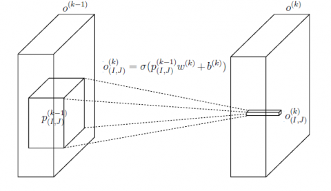
Each patch $Q_{(E, F)}^{(m-1)}$ defined by the outputs of the preceding layer exists for each brace of directories (E, F). To compute the set Q, the weight, the bias, and the activation function need to be applied to these coverings Q (m). On this account, it is possible to estimate the complexity of the convolution operation, which is visualized in Figure 1.
$\emptyset \mu_{\mathrm{m}}^{\mathrm{con}}=\emptyset\left(u_{m} V_{m M^{2}} n_{.}^{m-1 \times n_{\cdot}^{m}}\right)$
Figure 1. Visualization of convolution operation
3.2 Pooling
Like stride, pooling is a way to reduce the dimensionality of a layer’s width ( $U_{m}$) and height ( $V_{m}$) by reducing the number of sub-layers in the layer. There are various pooling techniques serving different objectives. Similarly to the convolution operation, pooling is compatible with patches $Q_{(E, F)(e)}^{(m-1)} \in S^{n X n}$. The only difference is that pooling uses simpler functions, instead of applying weight, bias, and activation function.
Max pooling considers the maximum in a channel within the patch. The first sub-index of a patch refers to a node defined as:
$Q_{(E, F)(e)}^{(m-1)} \in S^{n X n}, 0<e \leq n^{m-1}$
On this basis, max pooling can be defined as:
$\left.\mu_{\mathrm{m}}^{(\text {maxpool })} Q_{.}^{(m-1)}=Q^{m}=Q_{(E, F), e}^{(m-1)} / \forall(E, F), \mathrm{e}\right)\left(\exists Q_{(E, F), e}^{(m-1)}\right)$
$j_{(E, F), e}^{(m-1)}=\sum_{c=1}^{m} \sum_{d=1}^{m} \frac{Q_{(E, F) e, c . d}^{(m-1)}}{M^{2}}$
In other words, there is a M×M matrix for any index (E, F). The mean of a matrix refers to the output at index (E, F), e in the example above.
3.3 Fully connected layers
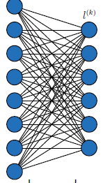
As its name suggests, fully connected layers link all the inputs from one layer to every activation unit of the next layer. In most fully connected layers, the bias is included to explain the system coefficients after completing a full connection operation. Figure 2 illustrates two fully connected layers.
The full convolution operation $\alpha_{m}^{G H}$ can be expressed as a function of the weight and the bias:
$j^{m}=\alpha_{m}^{G H} j^{(m-1)}=\left(j^{(m-1)}\right)^{S} U^{m}+C^{m}$
The computational complexity of $\alpha_{m}^{G H}$ can be obtained by:
$\mu\left(\alpha_{m}^{G H}\right)=\mu\left(n^{(m-1)} n^{(m)}\right)$
Figure 2. Two fully connected layers, $l^{(m-1)}$ and $l^{(m)}$, associated by $n^{(m)}$
3.4 Average pooling
Average pooling refers to the standards inside the covering per station. The sub-indices of covering $Q_{(E, F)}^{(m-1)}$ can be defined as:
$Q_{(E, F)(e, c, d)}^{(m-1)} \in S$
Thus, average pooling can be defined as:
$\left.\mu_{\mathrm{m}}^{(\text {avgpool })} Q_{.}^{(m-1)}=Q^{m}=Q_{(E, F), e}^{(m-1)} / \forall(E, F), \mathrm{e}\right)\left(\exists Q_{(E, F), e}^{(m-1)}\right)$
$j_{(E, F), e}^{(m-1)}=\sum_{c=1}^{m} \sum_{d=1}^{m} \frac{Q_{(E, F) e, c . d}^{(m-1)}}{M^{2}}$
That is, for every index (E, F), e, there exists an equivalent matrix of size m×m. When the output is at index (E, F), e, the value of the output is the mean the corresponding matrix.
4.1 Datasets
4.1.1 Dredze dataset
Wang and Cloete [4] developed an image spam dataset, which includes lots of original files in various formats, e.g., gif, txt, and jpg. The dataset was pre-processed to expand its size. Then, experiments were carried out using a mix of Dreze spam dataset and Dreze customised dataset. A subset of the latter dataset is the subjects of Wang and Cloete [1] and Baziotis et al. [6]. In total, the preprocessing produced 3,165 customised spam images, including 1,760 ham images, and 10,937 spam dataset images.
4.1.2 Image Spam Hunter (ISH) dataset
The ISH dataset contains both ham and spam images. For our experiments, 922 spam images and 820 ham images were extracted from the ISH dataset.
4.2 Performance metrics
True positive (TP) refer to the data points whose actual class is 1 (True), and projected class is also 1 (True).
True negative (TN) refer to the data points whose actual class is 0 (False), and projected class is also 0 (False).
False positive (FP) refer to the data points whose actual class is 0 (False), and projected class is 1 (True).
False negative (FN) refer to the data points whose actual class is 1 (True), and projected class is 0 (False).
Accuracy refers to the correct number of predictions out of total number of predictions.
Accuracy = True Positive / (True Positive+True Negative)*100
Precision refers to the ratio of TP to the sum of TP and FP.
Precision = TruePositives / (TruePositives + FalsePositives)
Recall refers to the ratio of TP to the sum of TP and FN. The correct identification, collection, and classification of image patterns (knowledge) depend on the recall.
Recall = TruePositives / (TruePositives + FalseNegatives)
F-score is the harmonic mean between precision and recall.
F-Measure = (2 * Precision * Recall) / (Precision + Recall)
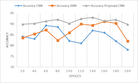
Figure 3. Accuracy on Dredze dataset
The detection accuracy of our model and several current models was tested on Dredze dataset. The results are reported in Figure 3. Obviously, our model was more accurate than the other models in the accuracy of detecting spam images in Dredze dataset.
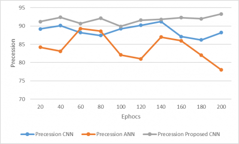
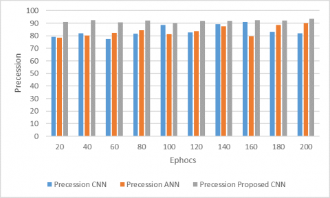
Figure 4. Precession on Dredze dataset
Figure 4 presents the precision of our model and several current models on Dredze dataset. It is clear that our model outshines the other models in the precision of detecting spam images in Dredze dataset.
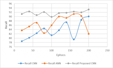
Figure 5. Recall on Dredze dataset
Figure 5 displays the recall of our model and several current models on Dredze dataset. It can be learned that our model worked better than the other models in the recall of detecting spam images in Dredze dataset.
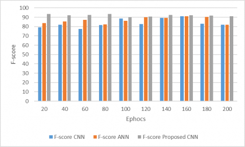
Figure 6. F-score on Dredze dataset
Figure 6 shows the F-measure of our model and several current models on Dredze dataset. It can be observed that our model did better than the other models in the F-measure of detecting spam images in Dredze dataset.
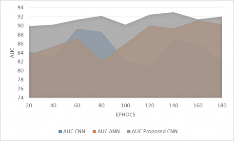
Figure 7. AUC on Dredze dataset
Figure 7 shows the area under the curve (AUC) of our model and several current models on Dredze dataset. It was found that the other models performed worse than our model in the AUC of detecting spam images in Dredze dataset.
Figure 8. Accuracy ISH dataset
Figure 9. Precession ISH dataset
Figures 8 and 9 shows the accuracy and precision of our model and several current models on ISH dataset. The two figures testify that our model realized the best performance in terms of accuracy and precision on various spam images in the dataset.
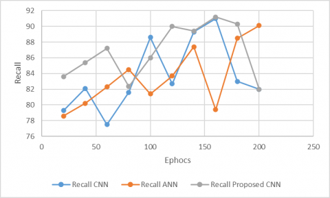
Figures 10 and 11 shows the recall and F-measure of our model and several current models on ISH dataset. The two figures reflect that our model surpassed the other models in terms of both measures on various spam images in the dataset.
Figure 10. Recall ISH dataset
Figure 11. F-score ISH dataset
Figure 12. AUC ISH dataset
Finally, Figure 12 shows the AUC of our model and several current models on ISH dataset. It is clear that our model accomplished the spam image detection task better than the other models.
Image spam is a hot topic among researchers. Many spam images are almost photo-quality images with various colours, and are composed of several photos. As a result, it is immensely difficult to classify spam images, not to mention differentiating between them and photos. This paper presents a powerful CNN-based classifier, and tests its performance on real-world spam image datasets. The CNN receives input in the form of images, and classifies them as spam or legitimate. Compared to state-of-the-art techniques, our model achieved an accuracy of nearly 98% and a FP of 0.03%. The future research will refine the algorithm, and create a comprehensive classification system, capable of identifying textual spam images.
[1] Wang X.L., Cloete. (2005). Learning to classify email: A survey. 2005 International Conference on Machine Learning and Cybernetics, pp. 5716-5719. https://doi.org/10.1109/ICMLC.2005.1527956
[2] Saad, O., Darwish, A., Faraj, R. (2012). A survey of machine learning techniques for spam filtering. International Journal of Computer Science and Network Security (IJCSNS), 12(2): 66-73.
[3] Kim, Y. (2014). Convolutional neural networks for sentence classification. Proceedings of the 2014 Conference on Empirical Methods in Natural Language Processing (EMNLP), pp. 1746-1751. https://doi.org/10.3115/v1/D14-1181
[4] Huang, Z., Xu, W., Yu, K. (2015). Bidirectional LSTM-CRF models for sequence tagging. arXiv preprint arXiv:1508.01991.
[5] Zhou, P., Shi, W., Tian, J., Qi, Z., Li, B., Hao, H., Xu, B. (2016). Attention-based bidirectional long short-term memory networks for relation classification. Proceedings of the 54th Annual Meeting of the Association for Computational Linguistics (Volume 2: Short Papers), pp. 207-212. https://doi.org/10.18653/v1/P16-2034
[6] Baziotis, C., Pelekis, N., Doulkeridis, C. (2017). DataStories at semeval-2017 task 4: Deep LSTM with attention for message-level and topic-based sentiment analysis. Proceedings of the 11th International Workshop on Semantic Evaluation (SemEval-2017), pp. 747-754. https://doi.org/10.18653/v1/S17-2126
[7] Devlin, J., Chang, M.W., Lee, K., Toutanova, K. (2018). Bert: Pre-training of deep bidirectional transformers for language understanding. Proceedings of the 2019 Conference of the North American Chapter of the Association for Computational Linguistics: Human Language Technologies, Volume 1 (Long and Short Papers), pp. 4171-4186. https://doi.org/10.18653/v1/N19-1423
[8] Narayana, V.L., Gopi, A.P., Khadherbhi, S.R., Pavani, V. (2020). Accurate identification and detection of outliers in networks using group random forest methodoly. Journal of Critical Reviews, 7(6): 381-384.
[9] Del Vigna, F., Cimino, A., Dell'Orletta, F., Petrocchi, M., Tesconi, M. (2017). Hate me, hate me not: Hate speech detection on Facebook. Proceedings of the First Italian Conference on Cybersecurity (ITASEC17), pp. 86-95.
[10] Srinivasan, S., Ravi, V., Alazab, M., Ketha, S., Al-Zoubi, A.M., Padannayil, S.K. (2021). Spam emails detection based on distributed word embedding with deep learning. In: Maleh Y., Shojafar M., Alazab M., Baddi Y. (eds) Machine Intelligence and Big Data Analytics for Cybersecurity Applications. Studies in Computational Intelligence, vol 919. Springer, Cham. https://doi.org/10.1007/978-3-030-57024-8_7
[11] Soni, A.N. (2019). Spam e-mail detection using advanced deep convolution neural network algorithms. Journal For Innovative Development in Pharmaceutical and Technical Science, 2(5): 74-80.
[12] Hassanpour, R., Dogdu, E., Choupani, R., Goker, O., Nazli, N. (2018). Phishing e-mail detection by using deep learning algorithms. Proceedings of the ACMSE 2018 Conference. https://doi.org/10.1145/3190645.3190719
[13] Egozi, G., Verma, R. (2018). Phishing email detection using robust NLP techniques. 2018 IEEE International Conference on Data Mining Workshops (ICDMW), pp. 7-12. https://doi.org/10.1109/ICDMW.2018.00009
[14] Seth, S., Biswas, S. (2017). Multimodal spam classification using deep learning techniques. 2017 13th International Conference on Signal-Image Technology & Internet-Based Systems (SITIS), pp. 346-349. https://doi.org/10.1109/SITIS.2017.91
[15] Ezpeleta, E., Zurutuza, U., Hidalgo, J.M.G. (2016). Does sentiment analysis help in Bayesian spam filtering? In: Martínez-Álvarez F., Troncoso A., Quintián H., Corchado E. (eds) Hybrid Artificial Intelligent Systems. HAIS 2016. Lecture Notes in Computer Science, vol 9648. Springer, Cham. https://doi.org/10.1007/978-3-319-32034-2_7
[16] Bibi, A., Latif, R., Khalid, S., Ahmed, W., Shabir, R.A., Shahryar, T. (2020). Spam mail scanning using machine learning algorithm. Journal of Computers, 15(2): 73-84. 2020. https://doi.org/10.17706/jcp.15.2.73-84
[17] Awad, W., ELseuofi, S. (2011). Machine learning methods for spam e-mail classification. International Journal of Computer Science & Information Technology (IJCSIT), 3(1): 173-184. https://doi.org/10.5121/ijcsit.2011.3112
[18] Saab, S.A., Mitri, N., Awad, M. (2014). Ham or spam? A comparative study for some content-based classification algorithms for email filtering. MELECON 2014-2014 17th IEEE Mediterranean Electrotechnical Conference, pp. 339-343. https://doi.org/10.1109/MELCON.2014.6820574
[19] Shajideen, N.M., Bindu, V. (2018). Spam filtering: A comparison between different machine learning classifiers. 2018 Second International Conference on Electronics, Communication and Aerospace Technology (ICECA), pp. 1919-1922. https://doi.org/10.1109/ICECA.2018.8474778
[20] Dua, D., Graff, C. UCI machine learning repository, 2017. [Online]. Available: http://archive.ics.uci.edu/ml, accessed on 12 June 2021.
[21] Veerakumar, K. Spam filter, 2017. [Online]. Available: https://www.kaggle.com/karthickveerakumar/spam-filter, accessed on 12 June 2021.
[22] Albon, C. (2018). Machine Learning with Python Cookbook: Practical Solutions from Preprocessing to Deep Learning. O'Reilly Media, Inc.
[23] Ketkar, N. (2017). Introduction to Keras. In: Deep Learning with Python. Apress, Berkeley, CA. https://doi.org/10.1007/978-1-4842-2766-4_7
[24] Liu, G., Guo, J. (2019). Bidirectional LSTM with attention mechanism and convolutional layer for text classification. Neurocomputing, 337: 325-338. https://doi.org/10.1016/j.neucom.2019.01.078
[25] Schmidt-Hieber, J. (2020). Nonparametric regression using deep neural networks with ReLU activation function. Annals of Statistics, 48(4): 1875-1897. https://doi.org/10.1214/19-AOS1875
[26] Hartmann, J., Huppertz, J., Schamp, C., Heitmann, M. (2019). Comparing automated text classification methods. International Journal of Research in Marketing, 36(1): 20-38. https://doi.org/10.1016/j.ijresmar.2018.09.009
[27] Tenney, I., Das, D., Pavlick, E. (2019). BERT rediscovers the classical NLP pipeline. Proceedings of the 57th Annual Meeting of the Association for Computational Linguistics, pp. 4593-4601. https://doi.org/10.18653/v1/P19-1452
[28] Rajapakse, T. [Online]. Available: https://simpletransformers.ai/, accessed on 12 June 2021.
[29] Wolf, T., Debut, L., Sanh, V., et al. (2019). Transformers: State-of-the-art natural language processing. Proceedings of the 2020 Conference on Empirical Methods in Natural Language Processing: System Demonstrations, pp. 38-45. https://doi.org/10.18653/v1/2020.emnlp-demos.6
[30] Zhu, Y., Kiros, R., Zemel, R., Salakhutdinov, R., Urtasun, R., Torralba, A., Fidler, S. (2015). Aligning books and movies: Towards story-like visual explanations by watching movies and reading books. 2015 IEEE International Conference on Computer Vision (ICCV), pp. 19-27. https://doi.org/10.1109/ICCV.2015.11
[31] Fan, G., Zhu, C., Zhu, W. (2019). Convolutional neural network with contextualized word embedding for text classification. 2019 International Conference on Image and Video Processing, and Artificial Intelligence, International Society for Optics and Photonics, 11321. https://doi.org/10.1117/12.2544614
[32] Gopi, A.P., Jairam Naik, K. (2021). A model for analysis of IoT based aquarium water quality data using CNN model. 2021 International Conference on Decision Aid Sciences and Application (DASA).