Lokesh Bhardwaj* | Ritesh Kumar Mishra
© 2022 IIETA. This article is published by IIETA and is licensed under the CC BY 4.0 license (http://creativecommons.org/licenses/by/4.0/).
OPEN ACCESS
This article shows the heterogeneous network of Massive Multiple-Input Multiple-Output (mMIMO) system and Non-Orthogonal Multiple Access (NOMA) scheme in Downlink (DL) scenario. The performance of mMIMO systems using Maximal Ratio Transmission (MRT) and Zero-Forcing (ZF) precoding techniques has been investigated and compared with mMIMO-NOMA systems. The problem of Pilot Contamination (PC) arises when the channel is estimated at the Base Station (BS) due to the reuse of the same pilot matrix in co-channel cells. To reduce the co-channel interference, it has been shown that the Cell Sectoring (CS) of 120 degree and 60 degree can be employed. Sum-Rate (SR) capacities have been derived for the mMIMO and the mMIMO-NOMA systems for un-sectored and sectored cells considering both Perfect Channel State Information (PCSI), and Imperfect Channel State Information (ICSI). In a multi-cell scenario, it has been shown that the mMIMO-NOMA system exploits the precoding advantage along with successive interference cancellation and outperforms the standalone mMIMO system. Further, the ZF precoded mMIMO-NOMA system with 60 degree CS has been observed to be the most appropriate candidate amongst all three systems viz. 120 degree CS, 60 degree CS, and un-sectored system in terms of reduced interference.
cell sectoring, channel state information, massive multiple-input multiple-output, non-orthogonal multiple access, pilot contamination, spectral efficiency
In this era of dynamic global communication, where the applications require high data rates, Spectral Efficiency (SE), very low latency, and high energy efficiency, the systems that can be employed to serve the said purposes are mMIMO and NOMA systems which has been explained by Chataut and Akl [1] and Ngo et al. [2]. To handle the increased data rates, multiple antennas are installed at the BS which can reduce the multi-user interference as well as the energy of the user mobile units. In the DL scenario, the segregated symbols of the users are precoded by the BS using MRT and ZF precoders for efficient reception by the user terminals. Zhang et al. [3] proposed an algorithm using which more spatial diversity gain has been employed using MRT precoding. Lv et al. [4] proposed an effective channel model which can increase the DL SE of mMIMO system having phase and thermal noise. Further, Sheikh et al. [5] proposed an efficient algorithm for user selection such as semi-orthogonal and random techniques with linear precoding which can maximize the SR capacity. Shalmashi et al. [6] demonstrated the increase in SR as the precoding gain is achieved with the increase in the BS antennas in DL. Isabona and Srivastava [7] proposed an energy-efficient system that employs non-linear successive interference cancellation precoding at the BS in DL for a microcellular environment. Further, You et al. [8] presented an algorithm based on the distribution of power which can reduce the inter-cell interference due to reduced signaling overhead that leads to limited sharing of information among the cells using the same resource. Jin et al. [9] introduced a technique using the beamforming training with MRT for improving the DL SR in multi-cell mMIMO systems. Boulouird et al. [10] suggested that the PC can erode the estimated channel due to the overlapping of pilot symbols, and hence, it reduces the performance of multi-cell mMIMO systems. Liu et al. [11] proposed a precoding scheme that is capable of reducing the interference when a considerably large number of antennas are used at the BS. Further, Bhardwaj and Mishra [12] proposed a scheme that can mitigate the effect of PC using low-density parity-check codes for improvement in the performance of multi-cell mMIMO in terms of SR, and bit error rate. Ashikhmin et al. [13] proposed a precoding scheme based on large-scale fading that is capable of eliminating the inter-cell interference through a linear combination of messages targeted for users from those cells that use the same pilot sequences. Zuo et al. [14] proposed a scheme-based on beamforming training and PC precoding for a multi-cell mMIMO system that can reduce the PC, and increase the SE through limited communication among the base stations. Hussain and Rasheed [15] studied that NOMA also increases the SE as the same resource is given to the multiple users present in a cell. Lim and Ko [16] proposed a user grouping scheme to reduce the degradation in the performance of NOMA caused due to an increase in the number of subscribers. Further, Zhang et al. [17] employed a stochastic approach to model a DL multi-cell wireless cellular system that uses the NOMA technique based on a group pairing scheme which provides considerable gain and SE. With power domain NOMA, SR increases as successive interference cancellation can mitigate the intra-cell interference in DL. Wang and Chen [18] suggested that the interference can be further reduced in DL NOMA networks through coordinated multi-point transmission, and load balancing that includes coordinated beamforming, and joint transmission techniques. Sun et al. [19] proposed a cluster-based grouping of users in which the user symbols are precoded with the same weighting factors depending on their location to enhance the SR. Sena et al. [20] proposed a mMIMO-NOMA scheme which can enhance the performance of the system if the power allocation coefficients are optimized under imperfect successive interference cancellation. Huang [21] proposed a mMIMO-NOMA scheme using the approach of random matrix theory for achieving SE, and energy efficiency in Fifth Generation (5G) communication systems. Mandawaria et al. [22] showed the improvement in the energy efficiency of mMIMO-NOMA systems by jointly allocating the power to multiple relays, and the BS of the cell. Further, Kudathanthirige and Baduge [23] showed the improvement in the SR for mMIMO-NOMA systems by reducing the effect of PC through the usage of linearly independent covariance matrices of those users who are sharing the pilot symbols in different clusters [23]. Hu et al. [24] proposed semi-blind Channel Estimation (CE) technique for mMIMO-NOMA systems which uses group successive interference cancellation assisted method to reduce the effect of PC in a multi-cell scenario. Ding and Cai [25] proposed a two-sided coalitional matching approach that is capable of enhancing the data rate through optimization of clustering, and BS selection in the mMIMO-NOMA system. Ali et al. [26] proposed that the SE gain can be achieved using NOMA in a multi-cell scenario through coordinated multipoint transmission in DL. Shahsavari et al. [27] proposed that sectoring in multi-cell mMIMO systems increases the data rate as the received signal power at the user terminal is increased, and the interference due to PC is decreased. Shankar et al. [28] proposed the integration of mMIMO and NOMA for a single cell for increasing the SE, and energy efficiency. Kudathanthirige and Amarasuriya [29] proposed a mMIMO-NOMA system by exploiting the pilot training in DL which enables the users to estimate their respective DL channels for implementation of successive interference cancellation. The mMIMO system includes a large antenna array at the BS due to which the small-scale fading effects can be easily averaged out resulting in the channel hardening. Further, signal processing by a simple matched filter is possible to reduce the complexity of the system. The interference among the users of the same cell reduces with an increase in the number of BS antennas. The mMIMO system enables the user devices to transmit the signals with less power.
On the other hand, NOMA is a main scheme to design a system based on radio access. The conceptualization of NOMA lies in providing an orthogonal resource to more than one user which makes NOMA a better scheme than Orthogonal Multiple Access technique (OMA). Thereby, SE increases in NOMA. However, merging NOMA with OMA such as orthogonal frequency division multiple access subcarriers can further improve its efficiency. NOMA also ensures fairness among the users as both strong and weak users can be served by the same bandwidth resource. So, NOMA provides a massive connectivity which is very crucial for Internet of Things usage in 5G and critical applications which require grant free access. The principle of successive interference cancellation in NOMA can reduce the interference at the weaker user terminal in DL and hence, this advantage has been exploited in this work to increase the SR of the users.
Based on the work done by the authors in the domain of mMIMO and NOMA systems, this paper has been drafted as follows: In section 2, the system model of the mMIMO-NOMA system for both single-cell, and sectored cell has been explained. In sections 3 and 4, models of mMIMO and mMIMO-NOMA systems in DL have been explained following which the modeling of un-sectored mMIMO and mMIMO-NOMA systems has been presented. In section 6, the proposed approach of 120° and 60° sectoring has been shown for both mMIMO and mMIMO-NOMA systems. The mMIMO-NOMA scheme is located in physical layer of 5G technology. The main challenge to be resolved is to overcome the effect of PC and the interference caused due to usage of same frequency in multi-cell scenario which has a consequential impact on the performance of 5G. The problem of interference seriously hampers the SINR at the user terminal which increases with the user base as well as with the number of cells using the same resource.
In this work, it has been shown that the interference received by a user in DL can be reduced using NOMA. However, the main novelty of this work studies the CS-based hybrid mMIMO-NOMA networks that can mitigate the co-channel interference in the presence of PC since less interfering power is received by a user from the co-channel BSs.
Contributions of the paper:
The system configuration of the mMIMO-NOMA network has been shown in Figure 1 for a single cell. Consider that there are two users U1 and U2 present in the cell who are receiving signals from the M BS antennas. The channel gain of U1 is less than U2 due to which U1 and U2 are considered as weak and strong users, respectively. Considering a1 and a2 as the symbols of U1 and U2, respectively, the power given to a1 is more than a2 due to difference in channel gains. The symbols a1 and a2 are then precoded using MRT and ZF precoding techniques for downlink transmission. The precoded symbols are linearly combined through superposition coding at the BS. Here, the superposition coding is implemented for power domain multiplexing. The resulting superposed symbols x1 x2 … xM are transmitted simultaneously by the corresponding transmitting antennas to U1 and U2 using the non-orthogonal resource.
The signals received by the users U1 and U2 are represented by y1 and y2, respectively. For precoding, the MRT and ZF precoders are considered as given below:
$\mathbf{R}=\mathbf{Q}^{*}$ for MRT (1)
$\mathbf{R}=\mathbf{Q} *\left(\mathbf{Q}^{T} \mathbf{Q}^{*}\right)^{-1}$ for ZF (2)
where, Q is the channel matrix between the users and the BS antennas.
Figure 1. Sum rate capacity of mMIMO-NOMA network for a single cell. U1 and U2 are weak and strong users, respectively
At U1 terminal, the symbol a1 is decoded considering the symbol a2 as interference. However, at U2 device, the symbol a1 is decoded first which is then removed through successive interference cancellation, and then a2 is decoded ensuring fairness among users. The rates corresponding to signal to interference ratio (SINR) at U1 and U2 terminals are given by R1 and R2. In a practical scenario, where multiple cells are given the same frequency for increasing the SE, users of the desired cell also receive the signals from the BS antennas of the interfering cells. The situation worsens when the number of co-channel cells increases. This number can be reduced by implementing CS where cells are divided into sectors of 120° and 60°. Figure 2 shows the general model of 120° CS where 7 sectors have the same frequency. S1, S2,…, S7 represent the co-channel sectors. Sector 1 (S1) is considered as the desired sector in which the BS antennas are receiving pilot symbols from the users present in all 7 sectors for (CE). PC arises due to the usage of the same pilot matrix in all sectors to reduce the overhead that degrades the performance as the estimated channel is erroneous. The estimated channel at every BS suffers from PC. However, the reception of interfering power by the users of S1 from the BS antennas of remaining co-channel sectors has been reduced in 120° sectoring as shown in Figure 3.
Figure 2. Channel estimation at the base station antennas of S1 in 120° sectoring. Dotted and bold arrows show the transmission of the same pilot symbols from the users of co-channel sectors and S1, respectively
The users of S1 are receiving the interfering power only from sector 2 (S2) and sector 3 (S3) which improves the performance of a multi-cell system. The coefficient qjm1irepresents the channel coefficient between the ith user of S1 and the mth BS antenna of the jth sector.
Figure 3. Signals received at the terminals of U1 and U2 in 120° sectoring
Figure 4 is depicting the scenario of 60° SC which further reduces the interference as S3 is the only sector from which interfering signals are received by the users of S1.
Figure 4. Signals received at the terminals of U1 and U2 in 60° sectoring
The system model presented in Figure 1 has been considered where the K×1 received signal vector is given in Eq. (3) [30].
$\mathbf{y}=\sqrt{\phi_{s}} \sqrt{p_{u}} \mathbf{Q}^{T} \mathbf{x}+\mathbf{n}=\sqrt{\phi_{s}} \sqrt{p_{u}}\left[\mathbf{q}_{1} \quad \mathbf{q}_{2}\right]^{T} \mathbf{x}+\mathbf{n}$ (3)
where, ϕs and pu represent the signal to noise ratio (SNR), and the average power given to the symbol of every user. q1 and q2 represent the channel vectors of U1 and U2, respectively.
n∼CN(0,1) is AWGN noise vector present at the user terminals. Further, the channel coefficient between the kth user and the mth antenna is qmk∼CN(0, ck), where E{qmk}=0 and $E\left\{\left|q_{m k}\right|^{2}\right\}=c_{k} \cdot c_{k}$. represents the large scaling fading that includes geometric attenuation, and shadow fading. The M×1 transmitted symbol vector from the BS is represented by x=Rb. Here R is a M×2 precoding matrix and b=$\left[\begin{array}{l}a_{1} \\ a_{2}\end{array}\right]$ is a 2×1 column vector having actual user symbols a1 and a2. The received signal y1 at U1 is given in Eq. (4).
$\begin{align} & {{y}_{1}}=\sqrt{{{\phi }_{s}}}\sqrt{{{p}_{u}}}{{\mathbf{q}}_{\mathbf{1}}}^{T}\mathbf{Rb}+{{n}_{1}} \\ & =\sqrt{{{\phi }_{s}}}\sqrt{{{p}_{u}}}{{\mathbf{q}}_{\mathbf{1}}}^{T}\left[ \begin{matrix} {{\mathbf{r}}_{\mathbf{1}}} & {{\mathbf{r}}_{\mathbf{2}}} \\ \end{matrix} \right]\mathbf{b}+{{n}_{1}} \\ \end{align}$ (4)
$=\sqrt{{{\phi }_{s}}}\sqrt{{{p}_{u}}}{{\mathbf{q}}_{\mathbf{1}}}^{T}{{\mathbf{r}}_{1}}{{a}_{1}}+\sqrt{{{\phi }_{s}}}\sqrt{{{p}_{u}}}{{\mathbf{q}}_{\mathbf{1}}}^{T}{{\mathbf{r}}_{\mathbf{2}}}{{a}_{2}}+{{n}_{1}}$ (5)
where, r1 and r2 are precoding vectors of U1 and U2, respectively.
SINR for U1 is thus given in Eq. (6).
$SIN{{R}_{U1}}=\frac{{{\phi }_{s}}{{p}_{u}}|{{\mathbf{q}}_{\mathbf{1}}}^{T}{{\mathbf{r}}_{1}}{{|}^{2}}}{{{\phi }_{s}}{{p}_{u}}|{{\mathbf{q}}_{\mathbf{1}}}^{T}{{\mathbf{r}}_{\mathbf{2}}}{{|}^{2}}+1}$ (6a)
Similarly, the SINR for U2 is
$SIN{{R}_{U2}}=\frac{{{\phi }_{s}}{{p}_{u}}|{{\mathbf{q}}_{\mathbf{2}}}^{T}{{\mathbf{r}}_{\mathbf{2}}}{{|}^{2}}}{{{\phi }_{s}}{{p}_{u}}|{{\mathbf{q}}_{\mathbf{2}}}^{T}{{\mathbf{r}}_{\mathbf{1}}}{{|}^{2}}+1}$ (6b)
The system shown in Figure 1 has been referred for the analysis. In power domain NOMA, the channel gain $\left|q_{1}\right|^{2}$ has been considered to be lesser than $\left|q_{2}\right|^{2}$ , so the power level P1 assigned to U1 is higher than the power level P2 given to U2. Here, $\left|q_{1}\right|^{2}$ and $\left|q_{2}\right|^{2}$ are the channel gains of U1 and U2, respectively.
The transmitted symbol from the $m^{t h}$ BS antenna as a result of superposition coding is given in Eq. (7).
${{x}_{m}}=\sqrt{{{p}_{1}}}\sqrt{{{\phi }_{s}}}{{a}_{1}}{{r}_{m1}}+\sqrt{{{p}_{2}}}\sqrt{{{\phi }_{s}}}{{a}_{2}}{{r}_{m2}}$ (7)
where, $r_{m i}$ is the element of precoding matrix R between the $i^{t h}$ user and the $m^{t h}$ BS antenna.
The received signal at the $i^{t h}$ user is given in Eq. (8).
${{y}_{i}}=\sum\limits_{j=1}^{M}{{{q}_{ji}}{{x}_{j}}}+{{n}_{i}}$, where i=1, 2 (8)
where, $q_{j i}$ is the channel coefficient between the $i^{t h}$ user and the $j^{t h}$ BS antenna.
$\Rightarrow y_{i}=\sum_{j=1}^{M} q_{j i}\left(\sqrt{p_{1}} \sqrt{\phi_{s}} a_{1} r_{j 1}+\sqrt{p_{2}} \sqrt{\phi_{s}} a_{2} r_{j 2}\right)+n_{i}$
$=\sum_{j=1}^{M} q_{j i} \sqrt{p_{1}} \sqrt{\phi_{s}} a_{1} r_{j 1}+\sum_{j=1}^{M} q_{j i} \sqrt{p_{2}} \sqrt{\phi_{s}} a_{2} r_{j 2}+n_{i}$ (9)
where, $\sum_{j=1}^{M} q_{j i} \sqrt{p_{2}} \sqrt{\phi_{s}} a_{2} r_{j 2}$ is the interfering part for the $i^{\text {th }}$ user in Eq. (9). As $U_{1}$ is the weak user, the symbol $a_{1}$ is decoded from the received signal as shown in Eq. (10).
$\begin{align} & {{y}_{1}}={{\mathbf{q}}_{\mathbf{1}}}^{T}\sqrt{{{p}_{1}}}\sqrt{{{\phi }_{s}}}{{a}_{1}}{{\mathbf{r}}_{1}} \\ & +{{\mathbf{q}}_{\mathbf{1}}}^{T}\sqrt{{{p}_{2}}}\sqrt{{{\phi }_{s}}}{{a}_{2}}{{\mathbf{r}}_{\mathbf{2}}}+{{n}_{1}} \\ \end{align}$ (10)
SINR for $U_{1}$ is thus given in Eq. (11).
$SIN{{R}_{U1}}=\frac{{{p}_{1}}{{\phi }_{s}}|{{\mathbf{q}}_{\mathbf{1}}}^{T}{{\mathbf{r}}_{1}}{{|}^{2}}}{{{p}_{2}}{{\phi }_{s}}|{{\mathbf{q}}_{\mathbf{1}}}^{T}{{\mathbf{r}}_{\mathbf{2}}}{{|}^{2}}+1}$ (11)
The received signal at $U_{2}$ is shown in Eq. (12) from which the symbol of $U_{1}$ is removed and then the desired symbol $a_{2}$ is decoded.
$\begin{align} & \Rightarrow {{y}_{2}}={{\mathbf{q}}_{\mathbf{2}}}^{T}\sqrt{{{p}_{2}}}\sqrt{{{\phi }_{s}}}{{a}_{2}}{{\mathbf{r}}_{\mathbf{2}}} \\ & +{{\mathbf{q}}_{\mathbf{2}}}^{T}\sqrt{{{p}_{1}}}\sqrt{{{\phi }_{s}}}{{a}_{1}}{{\mathbf{r}}_{\mathbf{1}}}+{{n}_{2}} \\ \end{align}$ (12)
After cancelling $a_{1}$, the signal and the corresponding SINR at $U_{2}$ have been shown in Eqns. (13) and (14), respectively.
$\Rightarrow {{y}_{2}}={{\mathbf{q}}_{\mathbf{2}}}^{T}\sqrt{{{p}_{2}}}\sqrt{{{\phi }_{s}}}{{a}_{2}}{{\mathbf{r}}_{\mathbf{2}}}+{{n}_{2}}$ (13)
$SIN{{R}_{U2}}={{p}_{2}}{{\phi }_{s}}|{{\mathbf{q}}_{\mathbf{2}}}^{T}{{\mathbf{r}}_{\mathbf{2}}}{{|}^{2}}$ (14)
Comparing Eqns. (6a), (6b) with Eqns. (11), (14), the SR has been found to be more for the later equations which makes the mMIMO-NOMA system perform better than the mMIMO system.
5.1 Downlink multi-cell massive MIMO system
In a multi-cell mMIMO system, multiple cells share the same frequency band. In this system, 7 cells have been considered in the first tier having 2 users in each cell. Further, the users of cell 1 are considered for the analysis, so the received signal vector at user terminals of cell 1 is given in Eq. (15).
${{\mathbf{y}}_{1}}=\sqrt{{{\phi }_{s}}}\sqrt{{{p}_{u}}}\sum\limits_{j=1}^{7}{{{\mathbf{Q}}_{j1}}^{T}}{{\mathbf{x}}_{j}}+{{\mathbf{n}}_{1}}$ (15)
where, $\boldsymbol{Q}_{j 1}$ represents the channel matrix between users of cell 1 and the BS antennas of the $j^{t h}$ cell. $\boldsymbol{x}_{j}=\boldsymbol{R}_{j j} \boldsymbol{b}_{j}$ represents the $M \times 1$ vector having transmitted symbols from the BS of the $j^{t h}$ cell. $\boldsymbol{R}_{j j}$ is the $M \times 2$ precoding matrix between the $j^{t h}$ cell users and the $j^{t h}$ cell BS. $b_{j}$ is the $2 \times 1$ column vector having user symbols of the $j^{t h}$ cell.
From Eq. (15), the received signal at $U_{1}$ in cell 1 is given in Eq. (16).
$y_{1}=\sqrt{\phi_{s}} \sqrt{p_{u}}$
$\left(\begin{array}{l}\mathbf{q}_{111}{ }^{T} \mathbf{R}_{11} \mathbf{b}_{1}+\mathbf{q}_{211}{ }^{T} \mathbf{R}_{22} \mathbf{b}_{2}+\mathbf{q}_{311}{ }^{T} \mathbf{R}_{33} \mathbf{b}_{3}+ \\ \mathbf{q}_{411}{ }^{T} \mathbf{R}_{44} \mathbf{b}_{4}+\mathbf{q}_{511}{ }^{T} \mathbf{R}_{55} \mathbf{b}_{5}+\mathbf{q}_{611}{ }^{T} \mathbf{R}_{66} \mathbf{b}_{6}+ \\ \mathbf{q}_{711}{ }^{T} \mathbf{R}_{77} \mathbf{b}_{7}\end{array}\right)+n_{1}$
$\begin{align} & \Rightarrow {{y}_{1}}=\sqrt{{{\phi }_{s}}}\sqrt{{{p}_{u}}} \\ & \left( \sum\limits_{j=1}^{7}{{{\mathbf{q}}_{j11}}^{T}}\left[ \begin{matrix} {{\mathbf{r}}_{jj1}} & {{\mathbf{r}}_{jj2}} \\ \end{matrix} \right]\left[ \begin{matrix} {{a}_{j1}} \\ {{a}_{j2}} \\ \end{matrix} \right] \right)+{{n}_{1}} \\ \end{align}$ (16)
where, $\boldsymbol{r}_{j j i}$ is the precoding vector between the $i^{t h}$ user of the $j^{t h}$ cell and the BS antennas of the $j^{t h}$ cell. $q_{j 1 i}$ is the channel vector between the $i^{t h}$ user of cell 1 and BS antennas of the $j^{t h}$ cell.
$\begin{align} & \Rightarrow {{y}_{1}}=\sqrt{{{\phi }_{s}}}\sqrt{{{p}_{u}}} \\ & \left( \sum\limits_{j=1}^{7}{{{\mathbf{q}}_{j11}}^{T}\left( {{\mathbf{r}}_{jj1}}{{a}_{j1}}+{{\mathbf{r}}_{jj2}}{{a}_{j2}} \right)} \right)+{{n}_{1}} \\ \end{align}$ (17)
Hence the SINR at $U_{1}$ of cell1 is given in Eq. (18).
$SIN{{R}_{U1}}=\frac{{{\phi }_{s}}{{p}_{u}}|{{\mathbf{q}}_{111}}^{T}{{\mathbf{r}}_{111}}{{|}^{2}}}{\begin{align} & {{\phi }_{s}}{{p}_{u}}|{{\mathbf{q}}_{111}}^{T}{{\mathbf{r}}_{112}}{{|}^{2}} \\ & +{{\phi }_{s}}{{p}_{u}}\sum\limits_{j=2}^{7}{\sum\limits_{i=1}^{2}{|{{\mathbf{q}}_{j11}}^{T}{{\mathbf{r}}_{jji}}{{|}^{2}}+1}} \\ \end{align}}$ (18)
where, $\boldsymbol{q}_{j 11}{ }^{T} \boldsymbol{r}_{j j i}$ is the interfering factor which represents the correlation between the channel vector of $U_{1}$ of cell 1 and the precoding vector of the $j^{t h}$ user of the $j^{t h}$ cell due to BS antennas of the $j^{t h}$ cell. Further, $\left|\boldsymbol{q}_{111}{ }^{T} \boldsymbol{r}_{112}\right|^{2}$ represents the interfering power at $U_{1}$ due to the precoding vector of $U_{2}$ of cell 1.
Similarly, the SINR at $U_{2}$of cell 1 is given in Eq. (19).
$SIN{{R}_{U2}}=\frac{{{\phi }_{s}}{{p}_{u}}|{{\mathbf{q}}_{112}}^{T}{{\mathbf{r}}_{112}}{{|}^{2}}}{\begin{align} & {{\phi }_{s}}{{p}_{u}}|{{\mathbf{q}}_{112}}^{T}{{\mathbf{r}}_{111}}{{|}^{2}} \\ & +{{\phi }_{s}}{{p}_{u}}\sum\limits_{j=2}^{7}{\sum\limits_{i=1}^{2}{|{{\mathbf{q}}_{j12}}^{T}{{\mathbf{r}}_{jji}}{{|}^{2}}+1}} \\ \end{align}}$ (19)
From Eqns. (18) and (19), it can be observed that the interfering power received at the user terminals of cell 1 is due to the transmission of signals from the 6 BS antennas.
5.2 Channel estimation
In the multi-cell system, every BS estimates the channel which is used for precoding the information. However, in data aided CE technique, the same pilot matrix is used in every cell to reduce the huge overhead that leads to PC. The CE model at cell 1 is given in Eq. (20).
$\mathbf{R}{{\mathbf{P}}_{1}}=\sqrt{{{P}_{pp}}}\sum\limits_{j=1}^{7}{{{\mathbf{F}}_{1j}}\mathbf{\Pi }}+{{\mathbf{N}}_{1}}$ (20)
where, $\boldsymbol{R} \boldsymbol{P}_{1}$ is the $M \times 2$ received matrix having pilot symbols at the BS of cell 1, and $F_{1 j}$ is also a $M \times 2$ channel matrix between the users of the $j^{t h}$ cell and the BS antennas of the cell 1. $\Pi$ is the $2 \times 2$ pilot matrix. $N_{1}$ is a noise matrix at the BS of cell 1. $P_{p p}$ is the power of the pilot matrix. Using the least-squares estimates, the estimated channel matrix at the BS of cell 1 is given in Eq. (21).
$\begin{align} & {{{\mathbf{\tilde{F}}}}_{11}}=\frac{1}{\sqrt{{{P}_{pp}}}}\mathbf{R}{{\mathbf{P}}_{1}}{{\mathbf{\Pi }}^{H}} \\ & =\frac{1}{\sqrt{{{P}_{pp}}}}(\sqrt{{{P}_{pp}}}\sum\limits_{j=1}^{7}{{{\mathbf{F}}_{1j}}}\mathbf{\Pi }+{{\mathbf{N}}_{1}}){{\mathbf{\Pi }}^{H}} \\ \end{align}$
$\begin{align} & =\sum\limits_{j=1}^{7}{{{\mathbf{F}}_{1j}}}+\frac{1}{\sqrt{{{P}_{pp}}}}{{\mathbf{N}}_{1}}{{\mathbf{\Pi }}^{H}} \\ & ={{\mathbf{F}}_{11}}+\sum\limits_{j=2}^{7}{{{\mathbf{F}}_{1j}}}+\frac{1}{\sqrt{{{P}_{pp}}}}{{\mathbf{N}}_{1}}{{\mathbf{\Pi }}^{H}} \\ \end{align}$ (21)
The estimated channel vector between user 1 and BS antennas of cell 1 is given in Eq. (22).
${{\mathbf{\tilde{f}}}_{111}}={{\mathbf{f}}_{111}}+\sum\limits_{j=2}^{7}{{{\mathbf{f}}_{1j1}}+{{{\mathbf{\tilde{n}}}}_{1}}}$ (22)
where, $\boldsymbol{f}_{1 j 1}$ is the channel vector corresponding to user 1 present in the $j^{t h}$ cell and the BS antennas of cell 1. Therefore, $\widetilde{f}_{111}$ is used in obtaining $\boldsymbol{r}_{111}$ for the calculation of SINR in (18).
Clearly $\sum_{j=2}^{7} f_{1 j 1}$ is the inter-cell interference due to PC. From Eq. (22), the desired estimated channel vector $\widetilde{f}_{111}$ also contains the channel vectors of user 1 present in the remaining 6 cells. This interference causes a huge problem as $\widetilde{f}_{111}$ will be used as the precoding vector for $U_{1}$ of cell 1. Further, $U_{1}$ of cell 1 also receives the signals from the BS antennas of 6 co-channel cells that add to interference caused due to PC. In a multi-cell system, this poses a challenge as SINR degrades with an increase in the number of cells.
5.3 Downlink multi-cell massive MIMO-NOMA system
In this system, $U_{1}$ and $U_{2}$ of every cell have been assumed as weak, and strong users, respectively. Therefore, the condition for assigning the power levels $p_{j 1}>p_{j 2}$ is uniform in every cell for all values of $j \cdot p_{j 1}$ and $p_{j 2}$ represent the power levels assigned to $U_{1}$ and $U_{2}$ of the $j^{t h}$ cell, respectively. The received signal model at the users of cell 1 is given in Eq. (23).
${{\mathbf{y}}_{1}}=\sqrt{{{\phi }_{s}}}\sum\limits_{j=1}^{7}{{{\mathbf{Q}}_{j1}}^{T}}{{\mathbf{x}}_{j}}+{{\mathbf{n}}_{1}}$ (23)
${{\mathbf{x}}_{j}}={{\mathbf{R}}_{jj}}{{\mathbf{b}}_{j}}=\left[ \begin{matrix} {{\mathbf{r}}_{jj1}} & {{\mathbf{r}}_{jj2}} \\ \end{matrix} \right]\left[ \begin{matrix} \sqrt{{{p}_{j1}}}{{a}_{j1}} \\ \sqrt{{{p}_{j2}}}{{a}_{j2}} \\ \end{matrix} \right]$ (24)
Referring to Eq. (17), the received signal at user 1 of cell 1 is given below:
$\Rightarrow {{y}_{1}}=\sqrt{{{\phi }_{s}}}\left( \sum\limits_{j=1}^{7}{{{\mathbf{q}}_{j11}}^{T}\left( \begin{align} & \sqrt{{{p}_{j1}}}{{\mathbf{r}}_{jj1}}{{a}_{j1}} \\ & +\sqrt{{{p}_{j2}}}{{\mathbf{r}}_{jj2}}{{a}_{j2}} \\ \end{align} \right)} \right)+{{n}_{1}}$ (25)
Thus, the SINR corresponding to $U_{1}$ of cell 1 is given in Eq. (26)
$SIN{{R}_{U1}}=\frac{{{\phi }_{s}}{{p}_{11}}|{{\mathbf{q}}_{111}}^{T}{{\mathbf{r}}_{111}}{{|}^{2}}}{\begin{align} & {{\phi }_{s}}{{p}_{12}}|{{\mathbf{q}}_{111}}^{T}{{\mathbf{r}}_{112}}{{|}^{2}} \\ & +{{\phi }_{s}}\sum\limits_{j=2}^{7}{{{p}_{j1}}|{{\mathbf{q}}_{j11}}^{T}{{\mathbf{r}}_{jj1}}{{|}^{2}}+} \\ & {{\phi }_{s}}\sum\limits_{j=2}^{7}{{{p}_{j2}}|{{\mathbf{q}}_{j11}}^{T}{{\mathbf{r}}_{jj2}}{{|}^{2}}+1} \\ \end{align}}$ (26)
The received signal at $U_{2}$ of cell 1 is given by:
$\Rightarrow {{y}_{2}}=\sqrt{{{\phi }_{s}}}\left( \sum\limits_{j=1}^{7}{{{\mathbf{q}}_{j12}}^{T}\left( \begin{align} & \sqrt{{{p}_{j1}}}{{\mathbf{r}}_{jj1}}{{a}_{j1}} \\ & +\sqrt{{{p}_{j2}}}{{\mathbf{r}}_{jj2}}{{a}_{j2}} \\ \end{align} \right)} \right)+{{n}_{2}}$ (27)
At $U_{2}$ terminal, the factor $\sqrt{p_{11}} \boldsymbol{q}_{112}{ }^{T} \boldsymbol{r}_{111} a_{11}$ corresponding to $U_{1}$ is removed as a part of the NOMA scheme and the resulting SINR is thus given in Eq. (28).
$SIN{{R}_{U2}}=\frac{{{\phi }_{s}}{{p}_{12}}|{{\mathbf{q}}_{112}}^{T}{{\mathbf{r}}_{112}}{{|}^{2}}}{{{\phi }_{s}}\sum\limits_{j=2}^{7}{\begin{align} & {{p}_{j1}}|{{\mathbf{q}}_{j12}}^{T}{{\mathbf{r}}_{jj1}}{{|}^{2}} \\ & +{{\phi }_{s}}\sum\limits_{j=2}^{7}{{{p}_{j2}}|{{\mathbf{q}}_{j12}}^{T}{{\mathbf{r}}_{jj2}}{{|}^{2}}+1} \\ \end{align}}}$ (28)
The SR due to Eqns. (27) and (28) yields better results than the SR due to Eqns. (18) and (19).
As $p_{11}>p_{12}$, the SINR in Eq. (26) is more than that of Eq. (18). Further, the factor corresponding to the interfering symbol of $U_{1}$ is canceled for calculating the SINR in Eq. (28) which results in increased SINR of $U_{2}$ as compared to SINR in Eq. (19).
The users of cell 1 under consideration receive the signals from all the 6 co-channel cells in an un-sectored system. However, in a CS system, the users present in a sector don’t receive the signals from all 6 sectors.
6.1 Multi-cell massive MIMO system with 120° sectoring
Considering the system having CS of 120° as shown in Figure 3, the number of interfering sectors is reduced to 2. Further, the CE at the desired sector 1 ($S_{1}$) considers the transmission of the pilot symbols from the users of all 6 co-channel sectors as shown in Figure 2. This means that the estimated channel vectors of $U_{1}$ and $U_{2}$ in $S_{1}$ contain the channel vectors of corresponding users of remaining co-channel sectors which has been explained in section 5.2.
The signal vector received at users of $S_{1}$ is given in Eq. (29).
${{\mathbf{y}}_{1}}=\sqrt{{{\phi }_{s}}}\sum\limits_{j=1}^{3}{{{{\mathbf{{Q}'}}}_{j1}}^{T}}{{\mathbf{{x}'}}_{j}}+{{\mathbf{n}}_{1}}$ (29)
where, $\boldsymbol{Q}_{j 1}^{\prime}$ represents the channel matrix between the users of $S_{1}$ and the BS antennas of the $j^{t h}$ sector. Also $\boldsymbol{x}_{j}^{\prime}=\boldsymbol{R}_{j j}^{\prime} \boldsymbol{b}_{j}^{\prime}$ represents the transmitted symbol vector from the BS antennas of the $j^{t h}$ sector.
The received signal at $U_{1}$ in $S_{1}$ is given in Eq. (30).
${{y}_{1}}=\sqrt{{{\phi }_{s}}}\sqrt{{{p}_{u}}}\left( \begin{align} & {{{\mathbf{{q}'}}}_{111}}^{T}{{{\mathbf{{R}'}}}_{11}}{{{\mathbf{{b}'}}}_{1}}+{{{\mathbf{{q}'}}}_{211}}^{T}{{{\mathbf{{R}'}}}_{22}}{{{\mathbf{{b}'}}}_{2}} \\ & +{{{\mathbf{{q}'}}}_{311}}^{T}{{{\mathbf{{R}'}}}_{33}}{{{\mathbf{{b}'}}}_{3}} \\ \end{align} \right)+{{n}_{1}}$ (30)
$\begin{align} & \Rightarrow {{y}_{1}}=\sqrt{{{\phi }_{s}}}\sqrt{{{p}_{u}}} \\ & \left( \sum\limits_{j=1}^{3}{{{{\mathbf{{q}'}}}_{j11}}^{T}}\left[ \begin{matrix} {{{\mathbf{{r}'}}}_{jj1}} & {{{\mathbf{{r}'}}}_{jj2}} \\ \end{matrix} \right]\left[ \begin{matrix} {{{{a}'}}_{j1}} \\ {{{{a}'}}_{j2}} \\ \end{matrix} \right] \right)+{{n}_{1}} \\ \end{align}$ (31)
$\Rightarrow y_{1}=\sqrt{\phi_{s}} \sqrt{p_{u}}$
$\left(\begin{array}{l}\mathbf{q}_{111}^{\prime}{ }^{T} \mathbf{r}_{111}^{\prime} a_{11}^{\prime}+\mathbf{q}_{111}^{\prime}{ }^{T} \mathbf{r}_{112}^{\prime} a_{12}^{\prime}+ \\ \mathbf{q}_{211}^{\prime}{ }^{T} \mathbf{r}_{221}^{\prime} a_{21}^{\prime}+\mathbf{q}_{211}^{\prime}{ }^{T} \mathbf{r}_{222}^{\prime} a_{22}^{\prime}+ \\ \mathbf{q}_{311}^{\prime}{ }^{T} \mathbf{r}_{331}^{\prime} a_{31}^{\prime}+\mathbf{q}_{311}^{\prime}{ }^{T} \mathbf{r}_{332}^{\prime} a_{32}^{\prime}\end{array}\right)+n_{1}$
where, $\boldsymbol{r}_{j j i}^{\prime}$ is the precoding vector between the $i^{t h}$ user of the $j^{t h}$ and the BS antennas of the $j^{t h}$ sector. $\boldsymbol{q}_{j 11}^{\prime}$ is the channel vector between $U_{1}$ of $S_{1}$ and $\mathrm{BS}$ antennas of the $j^{t h}$ sector. $a_{j i}^{\prime}$ represents the symbol of the$i^{t h}$ user present in the $j^{t h}$ sector.
Hence, the SINR at $U_{1}$ terminal of $S_{1}$ is given in Eq. (32).
$SIN{{R}_{U1}}=\frac{{{\phi }_{s}}{{p}_{u}}|{{{\mathbf{{q}'}}}_{111}}^{T}{{{\mathbf{{r}'}}}_{111}}{{|}^{2}}}{\begin{align} & {{\phi }_{s}}{{p}_{u}}|{{{\mathbf{{q}'}}}_{111}}^{T}{{{\mathbf{{r}'}}}_{112}}{{|}^{2}}+{{\phi }_{s}}{{p}_{u}}|{{{\mathbf{{q}'}}}_{211}}^{T}{{{\mathbf{{r}'}}}_{221}}{{|}^{2}}+ \\ & {{\phi }_{s}}{{p}_{u}}|{{{\mathbf{{q}'}}}_{211}}^{T}{{{\mathbf{{r}'}}}_{222}}{{|}^{2}}+{{\phi }_{s}}{{p}_{u}}|{{{\mathbf{{q}'}}}_{311}}^{T}{{{\mathbf{{r}'}}}_{331}}{{|}^{2}}+ \\ & {{\phi }_{s}}{{p}_{u}}|{{{\mathbf{{q}'}}}_{311}}^{T}{{{\mathbf{{r}'}}}_{332}}{{|}^{2}}+1 \\ \end{align}}$ (32)
Similarly, the SINR at $U_{2}$ terminal of $S_{1}$ is given in Eq. (33)
$SIN{{R}_{U2}}=\frac{{{\phi }_{s}}{{p}_{u}}|{{{\mathbf{{q}'}}}_{112}}^{T}{{{\mathbf{{r}'}}}_{112}}{{|}^{2}}}{\begin{align} & {{\phi }_{s}}{{p}_{u}}|{{{\mathbf{{q}'}}}_{112}}^{T}{{{\mathbf{{r}'}}}_{111}}{{|}^{2}}+{{\phi }_{s}}{{p}_{u}}|{{{\mathbf{{q}'}}}_{212}}^{T}{{{\mathbf{{r}'}}}_{221}}{{|}^{2}}+ \\ & {{\phi }_{s}}{{p}_{u}}|{{{\mathbf{{q}'}}}_{212}}^{T}{{{\mathbf{{r}'}}}_{222}}{{|}^{2}}+{{\phi }_{s}}{{p}_{u}}|{{{\mathbf{{q}'}}}_{312}}^{T}{{{\mathbf{{r}'}}}_{331}}{{|}^{2}}+ \\ & {{\phi }_{s}}{{p}_{u}}|{{{\mathbf{{q}'}}}_{312}}^{T}{{{\mathbf{{r}'}}}_{332}}{{|}^{2}}+1 \\ \end{align}}$ (33)
6.2 Multi-cell massive MIMO-NOMA system with 120° sectoring
The received signal model in Eq. (29) is referred for the 120° sectored mMIMO-NOMA system. The transmitted vector from BS antennas of the $j^{t h}$ sector is $\boldsymbol{x}_{j}^{\prime}=\boldsymbol{R}_{j j}^{\prime} \boldsymbol{b}_{j}^{\prime}=\left[\begin{array}{ll}\boldsymbol{r}_{j j 1}^{\prime} & \boldsymbol{r}_{j j 2}^{\prime}\end{array}\right]\left[\begin{array}{l}\sqrt{p_{j 1}^{\prime}} a_{j 1}^{\prime} \\ \sqrt{p_{j 2}^{\prime}} a_{j 2}^{\prime}\end{array}\right]$.
The received signal at $U_{1}$ terminal in $S_{1}$ is given in Eq. (34).
${{y}_{1}}=\sqrt{{{\phi }_{s}}}\left( \begin{align} & {{{\mathbf{{q}'}}}_{111}}^{T}{{{\mathbf{{R}'}}}_{11}}{{{\mathbf{{b}'}}}_{1}}+{{{\mathbf{{q}'}}}_{211}}^{T}{{{\mathbf{{R}'}}}_{22}}{{{\mathbf{{b}'}}}_{2}} \\ & +{{{\mathbf{{q}'}}}_{311}}^{T}{{{\mathbf{{R}'}}}_{33}}{{{\mathbf{{b}'}}}_{3}} \\ \end{align} \right)+{{n}_{1}}$ (34)
$\begin{align} & \Rightarrow {{y}_{1}}=\sqrt{{{\phi }_{s}}} \\ & \left( \sum\limits_{j=1}^{3}{{{{\mathbf{{q}'}}}_{j11}}^{T}}\left[ \begin{matrix} {{{\mathbf{{r}'}}}_{jj1}} & {{{\mathbf{{r}'}}}_{jj2}} \\ \end{matrix} \right]\left[ \begin{matrix} \sqrt{{{{{p}'}}_{j1}}}{{{{a}'}}_{j1}} \\ \sqrt{{{{{p}'}}_{j2}}}{{{{a}'}}_{j2}} \\ \end{matrix} \right] \right)+{{n}_{1}} \\ \end{align}$ (35)
$\Rightarrow y_{1}=\sqrt{\phi_{s}}$
$\left(\begin{array}{l}\sqrt{p_{11}^{\prime}} \mathbf{q}_{111}^{\prime} \mathbf{r}_{111}^{\prime} a_{11}^{\prime}+\sqrt{p_{12}^{\prime}} \mathbf{q}_{111}^{\prime} \mathbf{r}_{112}^{\prime} a_{12}^{\prime}+ \\ \sqrt{p_{21}^{\prime}} \mathbf{q}_{211}^{\prime} \mathbf{r}_{221}^{\prime} a_{21}^{\prime}+\sqrt{p_{22}^{\prime}} \mathbf{q}_{211}^{\prime} \mathbf{r}_{222}^{\prime} a_{22}^{\prime}+ \\ \sqrt{p_{31}^{\prime}} \mathbf{q}_{311}^{\prime}{ }^{T} \mathbf{r}_{331}^{\prime} a_{31}^{\prime}+\sqrt{p_{32}^{\prime}} \mathbf{q}_{311}^{\prime}{ }^{T} \mathbf{r}_{332}^{\prime} a_{32}^{\prime}\end{array}\right)+n_{1}$ (36)
where, $p_{j 1}^{\prime}$ and $p_{j 2}^{\prime}$ are the power levels assigned to $U_{1}$ and $U_{2}$ of the $j^{t h}$ sector. So, the SINR at $U_{1}$ terminal of $S_{1}$ is given in Eq. (37).
$SIN{{R}_{U1}}=\frac{{{\phi }_{s}}{{{{p}'}}_{11}}|{{{\mathbf{{q}'}}}_{111}}^{T}{{{\mathbf{{r}'}}}_{111}}{{|}^{2}}}{\begin{align} & {{\phi }_{s}}{{{{p}'}}_{12}}|{{{\mathbf{{q}'}}}_{111}}^{T}{{{\mathbf{{r}'}}}_{112}}{{|}^{2}} \\ & +{{\phi }_{s}}{{{{p}'}}_{21}}|{{{\mathbf{{q}'}}}_{211}}^{T}{{{\mathbf{{r}'}}}_{221}}{{|}^{2}} \\ & +{{\phi }_{s}}{{{{p}'}}_{22}}|{{{\mathbf{{q}'}}}_{211}}^{T}{{{\mathbf{{r}'}}}_{222}}{{|}^{2}} \\ & +{{\phi }_{s}}{{{{p}'}}_{31}}|{{{\mathbf{{q}'}}}_{311}}^{T}{{{\mathbf{{r}'}}}_{331}}{{|}^{2}} \\ & +{{\phi }_{s}}{{{{p}'}}_{32}}|{{{\mathbf{{q}'}}}_{311}}^{T}{{{\mathbf{{r}'}}}_{332}}{{|}^{2}}+1 \\ \end{align}}$ (37)
As $U_{1}$ is a weak user, $p_{11}^{\prime}>p_{12}^{\prime}$ due to which $a_{11}^{\prime}$ is decoded first whose SINR is given in Eq. (37). The symbol $a_{12}^{\prime}$ is decoded after the removal of the symbol $a_{11}^{\prime}$ from the received signal $y_{2}$ whose expression is given in Eq. (38).
$\Rightarrow y_{2}=\sqrt{\phi_{s}}$
$\left(\begin{array}{l}\sqrt{p_{11}^{\prime}} \mathbf{q}_{112}^{\prime} \mathbf{r}_{111}^{\prime} a_{11}^{\prime}+\sqrt{p_{12}^{\prime}} \mathbf{q}_{112}^{\prime}{ }^{T} \mathbf{r}_{112}^{\prime} a_{12}^{\prime}+ \\ \sqrt{p_{21}^{\prime}} \mathbf{q}_{212}^{\prime}{ }^{T} \mathbf{r}_{221}^{\prime} a_{21}^{\prime}+\sqrt{p_{22}^{\prime}} \mathbf{q}_{212}^{\prime}{ }^{T} \mathbf{r}_{222}^{\prime} a_{22}^{\prime}+ \\ \sqrt{p_{31}^{\prime}} \mathbf{q}_{312}^{\prime}{ }^{T} \mathbf{r}_{331}^{\prime} a_{31}^{\prime}+\sqrt{p_{32}^{\prime}} \mathbf{q}_{312}^{\prime}{ }^{T} \mathbf{r}_{332}^{\prime} a_{32}^{\prime}\end{array}\right)+n_{2}$ (38)
The factor $\sqrt{p_{11}^{\prime}} q_{112}^{\prime}{ }^{T} r_{111}^{\prime} a_{11}^{\prime}$ corresponding to $U_{1}$ of $S_{1}$ is removed at the terminal of $U_{2}$ of $S_{1}$, and the resulting SINR at $U_{2}$ is thus given in Eq. (39).
$SIN{{R}_{U2}}=\frac{{{\phi }_{s}}{{{{p}'}}_{12}}|{{{\mathbf{{q}'}}}_{112}}^{T}{{{\mathbf{{r}'}}}_{112}}{{|}^{2}}}{\begin{align} & {{\phi }_{s}}{{{{p}'}}_{21}}|{{{\mathbf{{q}'}}}_{212}}^{T}{{{\mathbf{{r}'}}}_{221}}{{|}^{2}} \\ & +{{\phi }_{s}}{{{{p}'}}_{22}}|{{{\mathbf{{q}'}}}_{212}}^{T}{{{\mathbf{{r}'}}}_{222}}{{|}^{2}} \\ & +{{\phi }_{s}}{{{{p}'}}_{31}}|{{{\mathbf{{q}'}}}_{312}}^{T}{{{\mathbf{{r}'}}}_{331}}{{|}^{2}} \\ & +{{\phi }_{s}}{{{{p}'}}_{32}}|{{{\mathbf{{q}'}}}_{312}}^{T}{{{\mathbf{{r}'}}}_{332}}{{|}^{2}}+1 \\ \end{align}}$ (39)
The SR obtained due to the SINRs in Eqns. (37) and (39) is inferred to be better than the SR due to SINRs in Eqns. (32) and (33). In Eq. (33), $a_{11}^{\prime}$ is providing interference to the SINR of $U_{2}$ while this interference is absent in Eq. (39).
6.3 Multi-cell massive MIMO system with 60° sectoring
Considering the system having CS of 60° as shown in Figure 4, the number of interfering sectors has been reduced to 1. The analysis of SR calculation is similar to the case of 120° sectoring as explained in section 6.1 except that now only ($S_{3}$) offers interference to the users of $S_{1}$. The signal vector received at users of $S_{1}$ is given in Eq. (40).
${{\mathbf{y}}_{1}}=\sqrt{{{\phi }_{s}}}\sqrt{{{p}_{u}}}\left( {{{\mathbf{{Q}'}}}_{11}}^{T}{{{\mathbf{{x}'}}}_{1}}+{{{\mathbf{{Q}'}}}_{31}}^{T}{{{\mathbf{{x}'}}}_{3}} \right)+{{\mathbf{n}}_{1}}$ (40)
$\Rightarrow \mathbf{y}_{1}=\sqrt{\phi_{s}} \sqrt{p_{u}}$
$\left(\begin{array}{l}\mathbf{Q}_{11}^{\prime T}\left[\begin{array}{ll}\mathbf{r}_{111}^{\prime} & \mathbf{r}_{12}^{\prime}\end{array}\right]\left[\begin{array}{l}a_{11}^{\prime} \\ a_{12}^{\prime}\end{array}\right]+ \\ \mathbf{Q}_{31}^{\prime T}\left[\begin{array}{ll}\mathbf{r}_{331}^{\prime} & \mathbf{r}_{332}^{\prime}\end{array}\right]\left[\begin{array}{l}a_{31}^{\prime} \\ a_{32}^{\prime}\end{array}\right]\end{array}\right)+n_{1}$ (41)
The signal received at user 1 is presented below:
${{y}_{1}}=\sqrt{{{\phi }_{s}}}\sqrt{{{p}_{u}}}\left( \begin{align} & {{{\mathbf{{q}'}}}_{111}}^{T}\left[ \begin{matrix} {{{\mathbf{{r}'}}}_{111}} & {{{\mathbf{{r}'}}}_{112}} \\ \end{matrix} \right]\left[ \begin{matrix} {{{{a}'}}_{11}} \\ {{{{a}'}}_{12}} \\ \end{matrix} \right]+ \\ & {{{\mathbf{{q}'}}}_{311}}^{T}\left[ \begin{matrix} {{{\mathbf{{r}'}}}_{331}} & {{{\mathbf{{r}'}}}_{332}} \\ \end{matrix} \right]\left[ \begin{matrix} {{{{a}'}}_{31}} \\ {{{{a}'}}_{32}} \\ \end{matrix} \right] \\ \end{align} \right)+{{n}_{1}}$ (42)
$\Rightarrow y_{1}=\sqrt{\phi_{s}} \sqrt{p_{u}}$
$\left(\begin{array}{l}\mathbf{q}_{111}^{\prime}{ }^{T} \mathbf{r}_{111}^{\prime} a_{11}^{\prime}+\mathbf{q}_{111}^{\prime}{ }^{T} \mathbf{r}_{112}^{\prime} a_{12}^{\prime}+ \\ \mathbf{q}_{311}^{\prime}{ }^{T} \mathbf{r}_{331}^{\prime} a_{31}^{\prime}+\mathbf{q}_{311}^{\prime}{ }^{T} \mathbf{r}_{332}^{\prime} a_{32}^{\prime}\end{array}\right)+n_{1}$ (43)
Hence the SINR at $U_{1}$ terminal of $S_{1}$ is given in Eq. (44).
$SIN{{R}_{U1}}=\frac{{{\phi }_{s}}{{p}_{u}}|{{{\mathbf{{q}'}}}_{111}}^{T}{{{\mathbf{{r}'}}}_{111}}{{|}^{2}}}{\begin{align} & {{\phi }_{s}}{{p}_{u}}|{{{\mathbf{{q}'}}}_{111}}^{T}{{{\mathbf{{r}'}}}_{112}}{{|}^{2}} \\ & +{{\phi }_{s}}{{p}_{u}}|{{{\mathbf{{q}'}}}_{311}}^{T}{{{\mathbf{{r}'}}}_{331}}{{|}^{2}} \\ & +{{\phi }_{s}}{{p}_{u}}|{{{\mathbf{{q}'}}}_{311}}^{T}{{{\mathbf{{r}'}}}_{332}}{{|}^{2}}+1 \\ \end{align}}$ (44)
Similarly, the SINR corresponding to $U_{2}$ terminal of $S_{1}$ is given in Eq. (45).
$SIN{{R}_{U2}}=\frac{{{\phi }_{s}}{{p}_{u}}|{{{\mathbf{{q}'}}}_{112}}^{T}{{{\mathbf{{r}'}}}_{112}}{{|}^{2}}}{\begin{align} & {{\phi }_{s}}{{p}_{u}}|{{{\mathbf{{q}'}}}_{112}}^{T}{{{\mathbf{{r}'}}}_{111}}{{|}^{2}} \\ & +{{\phi }_{s}}{{p}_{u}}|{{{\mathbf{{q}'}}}_{312}}^{T}{{{\mathbf{{r}'}}}_{331}}{{|}^{2}} \\ & +{{\phi }_{s}}{{p}_{u}}|{{{\mathbf{{q}'}}}_{312}}^{T}{{{\mathbf{{r}'}}}_{332}}{{|}^{2}}+1 \\ \end{align}}$ (45)
From Eqns. (44) and (45), the reduction in the interference has been observed if compared with the SINRs given in Eqns. (32) and (33) for 120° sectoring.
6.4 Multi-cell massive MIMO-NOMA system with 60° sectoring
It has already been discussed that $S_{3}$ is the only interferer for the users of $S_{1}$. Modifying Eq. (42), the received signal at $U_{1}$ of $S_{1}$ is given in Eq. (46).
$\Rightarrow y_{1}=\sqrt{\phi_{s}}$
$\left(\begin{array}{l}\mathbf{q}_{111}^{\prime}{ }^{T}\left[\begin{array}{ll}\mathbf{r}_{111}^{\prime} & \mathbf{r}_{112}^{\prime}\end{array}\right]\left[\begin{array}{c}\sqrt{p_{11}^{\prime}} a_{11}^{\prime} \\ \sqrt{p_{12}^{\prime}} a_{12}^{\prime}\end{array}\right]+ \\ \mathbf{q}_{311}^{\prime}{ }^{T}\left[\begin{array}{ll}\mathbf{r}_{331}^{\prime} & \mathbf{r}_{332}^{\prime}\end{array}\right]\left[\begin{array}{c}\sqrt{p_{31}^{\prime}} a_{31}^{\prime} \\ \sqrt{p_{32}^{\prime}} a_{32}^{\prime}\end{array}\right]\end{array}\right)+n_{1}$ (46)
$\Rightarrow y_{1}=\sqrt{\phi_{s}}$
$\left(\begin{array}{c}\sqrt{p_{11}^{\prime}} \mathbf{q}_{111}^{\prime}{ }^{T} \mathbf{r}_{111}^{\prime} a_{11}^{\prime}+\sqrt{p_{12}^{\prime}} \mathbf{q}_{111}^{\prime}{ }^{T} \mathbf{r}_{112}^{\prime} a_{12}^{\prime}+ \\ \sqrt{p_{31}^{\prime}} \mathbf{q}_{311}^{\prime}{ }^{T} \mathbf{r}_{331}^{\prime} a_{31}^{\prime}+\sqrt{p_{32}^{\prime}} \mathbf{q}_{311}^{\prime}{ }^{T} \mathbf{r}_{332}^{\prime} a_{32}^{\prime}\end{array}\right)+n_{1}$ (47)
SINR at $U_{1}$ of $S_{1}$ is given in Eq. (48).
$SIN{{R}_{U1}}=\frac{{{\phi }_{s}}{{{{p}'}}_{11}}|{{{\mathbf{{q}'}}}_{111}}^{T}{{{\mathbf{{r}'}}}_{111}}{{|}^{2}}}{\begin{align} & {{\phi }_{s}}{{{{p}'}}_{12}}|{{{\mathbf{{q}'}}}_{111}}^{T}{{{\mathbf{{r}'}}}_{112}}{{|}^{2}}+{{\phi }_{s}}{{{{p}'}}_{31}}|{{{\mathbf{{q}'}}}_{311}}^{T}{{{\mathbf{{r}'}}}_{331}}{{|}^{2}}+ \\ & {{\phi }_{s}}{{{{p}'}}_{32}}|{{{\mathbf{{q}'}}}_{311}}^{T}{{{\mathbf{{r}'}}}_{332}}{{|}^{2}}+1 \\ \end{align}}$ (48)
The symbol of $U_{1}$ is then decoded and removed at $U_{2}$ terminal. The expression of the received signal at $U_{2}$ is given below:
$\Rightarrow y_{2}=\sqrt{\phi_{s}}$
$\left(\begin{array}{l}\sqrt{p_{11}^{\prime}} \mathbf{q}_{112}^{\prime}{ }^{T} \mathbf{r}_{111}^{\prime} a_{11}^{\prime}+\sqrt{p_{12}^{\prime}} \mathbf{q}_{112}^{\prime}{ }^{T} \mathbf{r}_{112}^{\prime} a_{12}^{\prime}+ \\ \sqrt{p_{31}^{\prime}} \mathbf{q}_{312}^{\prime}{ }^{T} \mathbf{r}_{331}^{\prime} a_{31}^{\prime}+\sqrt{p_{32}^{\prime}} \mathbf{q}_{312}^{\prime}{ }^{T} \mathbf{r}_{332}^{\prime} a_{32}^{\prime}\end{array}\right)+n_{2}$ (49)
Now the factor $\sqrt{p_{11}^{\prime}} q_{112}^{\prime}{ }^{T} r_{111}^{\prime} a_{11}^{\prime}$ is removed at $U_{2}$ terminal of $S_{1}$, and the SINR corresponding to $U_{2}$ is thus given in Eq. (50).
$SIN{{R}_{U2}}=\frac{{{\phi }_{s}}{{{{p}'}}_{12}}|{{{\mathbf{{q}'}}}_{112}}^{T}{{{\mathbf{{r}'}}}_{112}}{{|}^{2}}}{\begin{align} & {{\phi }_{s}}{{{{p}'}}_{31}}|{{{\mathbf{{q}'}}}_{312}}^{T}{{{\mathbf{{r}'}}}_{331}}{{|}^{2}} \\ & +{{\phi }_{s}}{{{{p}'}}_{32}}|{{{\mathbf{{q}'}}}_{312}}^{T}{{{\mathbf{{r}'}}}_{332}}{{|}^{2}}+1 \\ \end{align}}$ (50)
Clearly, there are only two interfering factors in Eq. (50) as compared to the interfering factors in Eqns. (28) and (39). Hence the SR of the 60° CS mMIMO-NOMA system is found to be better than the 120° CS and un-sectored counterparts.
Algorithm: Sum-rate of Massive MIMO-NOMA system for sectored cells having ICSI
Initialize:
iter, $n_{R X}, n_{T X}, S N R, c a p, s_{u 1}, s_{u 2}$; number of iterations, number of receive antennas in a sector, number of transmit antennas in a sector, SNR range, capacity range, power levels of user 1 and user 2 respectively in a sector.
for it $=1:$ iter
for $i x=1: S N R$
for $k=1: 2$
end
end
end
$c a p=c a p / i t e r$
The results obtained for multi-cell mMIMO and multi-cell mMIMO-NOMA systems in DL have been discussed in this section. The MRT and ZF precoders have been used in forming the symbol vectors for the transmission from the BS to the users. First, the un-sectored case has been considered where the desired cell 1 is surrounded by 6 co-channel cells.
If BS of cell 1 has PCSI then the precoding vectors for $U_{1}$ and $U_{2}$ are $\boldsymbol{h}_{111}$ and $\boldsymbol{h}_{112}$, respectively. Here $\boldsymbol{h}_{111}$ is the actual channel vector between $U_{1}$ and the BS antennas of cell 1. The results have been obtained for 50 BS antennas, and the average power of 0.5 has been given to every user. Further, these users also receive the signals from the BS of the remaining 6 cells. For the mMIMO system, the variation in SR with SNR for PCSI has been shown in Figure 5.
The mMIMO-NOMA system improves the SR due to successive interference cancellation at the stronger user, and hence, this improvement is depicted in Figure 6.
At the BS, the power levels assigned to the symbols of $U_{1}$ and $U_{2}$ are 0.7 and 0.3 since the channel gains of $U_{1}$ and $U_{2}$ are 7 and 10, respectively. The MRT precoder performs better for low values of SNR while the rise in SR is limited by a further increase in SNR. ZF precoder has more ability to neutralize the multi-user interference. Considering the ICSI at the BS, the PC degrades the performance of both mMIMO and mMIMO-NOMA systems. The result of PC has a serious impact on the SINR at the user terminals. As the number of interferers in the un-sectored scenario is 6, the situation further worsens, and the variations in SRs with SNR have been shown in Figure 7 and Figure 8.
Figure 5. Sum rate of the un-sectored mMIMO system having PCSI
Figure 6. Sum rate of the un-sectored mMIMO-NOMA system having PCSI
Figure 7. Sum rate of the un-sectored mMIMO system having ICSI
From Figure 8, it can be seen that the SR improves for the mMIMO-NOMA system. However, the improvement in both systems can be further enhanced if the CS approach is employed where the number of interfering sectors can be reduced. The variation in SR for 120° CS for mMIMO and mMIMO-NOMA systems has been shown in Figure 9 and Figure 10, respectively for PCSI.
Figure 8. Sum rate of the un-sectored mMIMO-NOMA having ICSI
Figure 9. Sum rate of the 120° sectored mMIMO system having PCSI
Figure 10. Sum rate of the 120° sectored mMIMO-NOMA having PCSI
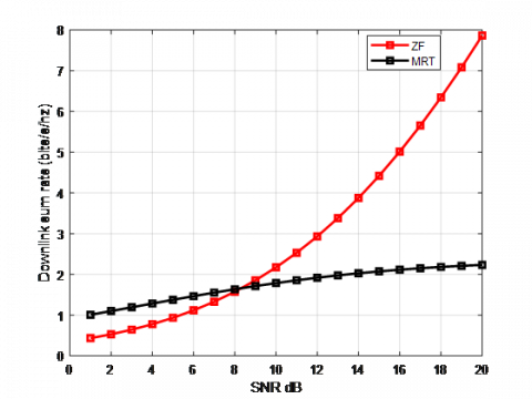
The SR in Figure 9 for ZF precoding increases by 3 times the SR shown in Figure 5 since the number of interferes for Figure 9 has now been reduced to 2. For MRT precoding, there is an increase by a factor of 2 for 120° sectoring in Figure 9. Further, the SR reduces with ICSI at the BS which has been depicted in Figures 11 and 12 for mMIMO and mMIMO-NOMA systems, respectively.
Figure 11. Sum rate of the 120° sectored mMIMO system having ICSI
Figure 12. Sum rate of the 120° sectored mMIMO-NOMA system having ICSI
Figure 13. Sum rate of the 60° sectored mMIMO system having PCSI
Figure 14. Sum rate of the 60° sectored mMIMO-NOMA system having PCSI
Figure 15. Sum rate of the 60° sectored mMIMO system having ICSI
Figure 16. Sum rate of the 60° sectored mMIMO-NOMA system having ICSI
From Figures 9-12, it is visible that the sectoring has increased the SINR. However, a high data rate is required in next-generation 5G technology for which CS of 60° can be employed.
Table 1. Maximum SR for un-sectored and sectored approaches with PCSI and ICSI for MRT and ZF precoders in mMIMO and mMIMO-NOMA systems
|
|
Maximum SR (bits/sec/Hz) |
|||
|
Approach |
MRT for PCSI |
MRT for ICSI |
ZF for PCSI |
ZF for ICSI |
|
Un-sectored (mMIMO) |
0.94 |
0.48 |
1.35 |
1.23 |
|
Un-sectored (mMIMO-NOMA) |
2.04 |
0.6 |
2.24 |
1.6 |
|
120° sectored (mMIMO) |
2.1 |
1 |
4.2 |
3.6 |
|
120° sectored (mMIMO-NOMA) |
3.7 |
1.1 |
4.4 |
5 |
|
60° sectored (mMIMO) |
2.2 |
1.4 |
8 |
4.8 |
|
60° sectored (mMIMO-NOMA) |
4.1 |
2.1 |
9.2 |
8 |
The frequency reuse in all the co-channel sectors also introduces the PC in 60° CS while estimating the channel but the number of interfering sectors is now reduced to 1. For 60° CS, the variation in the SR with SNR for mMIMO and mMIMO-NOMA systems has been shown in Figures 13 and 14 and Figures 15 and 16, respectively.
Table 1 shows the summary of the variation in SR with SNR for mMIMO and mMIMO-NOMA systems for un-sectored, 120° CS, and 60° CS approaches with PCSI and ICSI at the BS.
From Table 1, ZF overpowers the MRT precoder in all the approaches. Further, the mMIMO-NOMA system performs better than the mMIMO system. It can also be observed that there is an improvement of 3.4 bits/sec/Hz and 6.4 bits/sec/Hz in 120° and 60° CS mMIMO-NOMA systems, respectively, if compared with the un-sectored counterpart.
The article has studied the SR capacities of standalone mMIMO and mMIMO-NOMA systems for un-sectored and CS approaches. In mMIMO systems, SE increases as the same frequency can be used for multiple users in a cell. Further, SR of mMIMO systems can be increased if NOMA is also implemented simultaneously in the same cell. With the increase in the user base, the same frequency band is required to be allocated in the multiple cells but this increase in the SE comes at the cost of PC which reduces the performance of mMIMO-NOMA systems. In a multi-cell scenario, the interfering power received from the co-channel BSs at the users of the desired cell increases with an increase in the number of co-channel cells. This interfering power along with the interference due to PC seriously hampers the performance of both mMIMO and mMIMO-NOMA systems. It has been shown that if CS is employed, mMIMO-NOMA systems perform much better even under ICSI conditions. With 120° CS, the SR of mMIMO-NOMA systems has been observed to be thrice and, with 60° CS it is four times the SR of the un-sectored case when ZF precoder is used at the BS. Further, MRT can be employed for low SNRs and is useful for the CS of 60°. Finally, it can be concluded that the sectored mMIMO-NOMA systems can control the interference received by the users in a multi-cell scenario in presence of PC.
Further, SR can be enhanced if the techniques related to mitigation of PC can be employed as the interference free CE at the BS is a challenging task in a multi-cell scenario. So, the future work for this study is to obtain the SR capacities of mMIMO-NOMA systems using CS in the absence of PC.
Another optimization direction of the work done in this paper is to increase the number of users that could be served by the BSs since, CS reduces the coverage area of BSs thereby, lower number of users is accommodated by the BSs. So, the desired outcome can be hampered and there is a tradeoff here. The number of channels given to a cell in a cluster can be used by the users present anywhere in the coverage area of that cell if the un-sectored system is considered. However, the same number of channels in that cell is divided into a group of 3 and 6 for CS of 120° and 60° respectively. This results in a reduced number of channels for users present in any sector. Therefore, the trunking efficiency gets reduced in the case of CS. However, due to CS, the interference experienced by a user also gets reduced. The minimum SINR for a user should be approximately 18 dB, and with this SINR, the interference is within tolerable limits. Due to CS, the SINR gets increased for a user due to which the cluster size can be reduced keeping the cell size constant. The reduced cluster size results in the allotment of more channels to a cell that further leads to an increased number of channels in the sectors as well. Thus, the reduction of the interference due to CS leads to increase in the capacity of the system to some extent. Hence, there is a tradeoff between the capacity and the interference.
mMIMO technology can be widely used in cellular communications and real time applications such as vehicle to vehicle communications where signal processing with ultra-low latency is pivotal. In such applications, the data rate required is enormous which justifies the work done in this paper as the SR enhancement has been proposed for mMIMO systems using NOMA scheme for CS approach which can reduce the interference thereby, increasing the data rates for the end users.
[1] Chataut, R., Akl, R. (2020). Massive MIMO systems for 5G and beyond networks—overview, recent trends, challenges, and future research direction. Sensors, 20(10): 2753. https://doi.org/10.3390/s20102753
[2] Ngo, H.Q., Larsson, E.G., Marzetta, T.L. (2013). Energy and spectral efficiency of very large multiuser MIMO systems. IEEE Transactions on Communications, 61(4): 1436-1449. https://doi.org/10.1109/TCOMM.2013.020413.110848
[3] Zhang, Y., Gao, J., Liu, Y. (2016). MRT precoding in downlink multi-user MIMO systems. EURASIP Journal on Wireless Communications and Networking, 2016(1): 1-7. https://doi.org/10.1186/s 13638-016- 0738-6
[4] Lv, Q., Li, J., Zhu, P., Wang, D., You, X. (2018). Downlink spectral efficiency analysis in distributed massive MIMO with phase noise. Electronics, 7(11): 317. https://doi.org/10.3390/electronics7110317
[5] Sheikh, T.A., Bora, J., Hussain, M. (2021). Capacity maximizing in massive MIMO with linear precoding for SSF and LSF channel with perfect CSI. Digital Communications and Networks, 7(1): 92-99. https://doi.org/10.1016/j.dcan.2019.08.002
[6] Shalmashi, S., Björnson, E., Kountouris, M., Sung, K.W., Debbah, M. (2016). Energy efficiency and sum rate tradeoffs for massive MIMO systems with underlaid device-to-device communications. EURASIP Journal on wireless Communications and Networking, 2016(1): 1-18. https://doi.org/10.1186/ s13638-016-0678-1
[7] Isabona, J., Srivastava, V.M. (2017). Downlink massive MIMO systems: Achievable sum rates and energy efficiency perspective for future 5G systems. Wireless Personal Communications, 96(2): 2779-2796. https://doi.org/10.1007/s11277-017-4324-y
[8] You. L., Huang. Y., Zhang. D., Chang. Z., Wang. W., Gao. X. (2021). Energy efficiency optimization for multi-cell massive MIMO: Centralized and distributed power allocation algorithms. IEEE Transactions on Communications, 69(8): 5228-5242. https://doi.org/10.1109/TCOMM.2021.3081451
[9] Jin, S., Yue, D., Nguyen, H.H. (2019). Multicell massive MIMO: Downlink rate analysis with linear processing under Ricean fading. IEEE Transactions on Vehicular Technology, 68(4): 3777-3791. https://doi.org/10.1109/TVT.2019.2902014
[10] Boulouird, M., Riadi, A., Hassani, M.M. (2017). Pilot contamination in multi-cell massive-MIMO systems in 5G wireless communications. International Conference on Electrical and Information Technologies (ICEIT), Rabat, Morocco, Russia, pp. 1-4. https://doi.org/10.1109/EITech. 2017.8255299
[11] Liu, B., Cheng, Y., Yuan, X. (2015). Pilot contamination elimination precoding in multi-cell massive MIMO systems. IEEE 26th Annual International Symposium on Personal, Indoor, and Mobile Radio Communications (PIMRC), Hong Kong, pp. 320-325. https://doi.org/10.1109/PIMRC.2015.7343317
[12] Bhardwaj, L., Mishra, R.K. (2020). Mitigating the interference caused by pilot contamination in multi-cell massive multiple input multiple output systems using low density parity check codes in uplink scenario. Traitement du Signal, 37(6): 1061-1074. https://doi.org/10.18280/ts.370619
[13] Ashikhmin, A., Li, L., Marzetta, T.L. (2018). Interference reduction in multi-cell massive MIMO systems with large-scale fading precoding. IEEE Transactions on Information Theory, 64(9): 6340-6361. https://doi.org/10.1109/TIT.2018.2853733
[14] Zuo, J., Zhang, J., Yuen, C., Jiang, W., Luo, W. (2015). Multicell multiuser massive MIMO transmission with downlink training and pilot contamination precoding. IEEE Transactions on Vehicular Technology, 65(8): 6301-6314. https://doi.org/ 10.1109/TVT.2015.2475284
[15] Hussain, M., Rasheed, H. (2020). Nonorthogonal multiple access for next-generation mobile networks: A technical aspect for research direction. Wireless Communications and Mobile Computing. https://doi.org/10.1155/2020/8845371
[16] Lim, S., Ko, K. (2015). Non-orthogonal multiple access (NOMA) to enhance capacity in 5G. International Journal of Contents, 11(4): 38-43. https://doi.org/10.5392/IJoC.2015.11.4.038
[17] Zhang, Z., Sun, H., Hu, R.Q. (2017). Downlink and uplink non-orthogonal multiple access in a dense wireless network. IEEE Journal on Selected Areas in Communications, 35(12): 771-2784. https://doi.org/10.1109/JSAC.2017.2724646
[18] Wang, X., Chen, Y. (2017). An effective interference mitigation scheme for downlink NOMA heterogeneous networks. In 2017 3rd IEEE International Conference on Computer and Communications (ICCC), pp. 384-388. https://doi.org/10.1109/CompComm.2017.8322576
[19] Sun, X., Duran-Herrmann, D., Zhong, Z., Yang, Y. (2015). Non-orthogonal multiple access with weighted sum-rate optimization for downlink broadcast channel. In MILCOM 2015-2015 IEEE Military Communications Conference, pp. 1176-1181. https://doi.org/10.1109/MILCOM.2015.7357605
[20] de Sena, A.S., Lima, F.R.M., da Costa, D.B., Ding, Z., Nardelli, P.H., Dias, U.S., Papadias, C.B. (2020). Massive MIMO-NOMA networks with imperfect SIC: Design and fairness enhancement. IEEE Transactions on Wireless Communications, 19(9): 6100-6115. https://doi.org/ 10.1109/TWC.2020.3000192
[21] Huang, T.J. (2020). Theoretical analysis of NOMA within massive MIMO systems. Wireless Personal Communications, 112(2): 777-783. https://doi.org/10.1007/s11277 -020-07073-z
[22] Mandawaria, V., Sharma, E., Budhiraja, R. (2020). Energy-efficient massive MIMO multi-relay NOMA systems with CSI errors. IEEE Transactions on Communications, 68(12): 7410-7428. https://doi.org/10.1109/ TCOMM.2020.3019316
[23] Kudathanthirige, D., Baduge, G.A.A. (2019). NOMA-aided multicell downlink massive MIMO. IEEE Journal of Selected Topics in Signal Processing, 13(3): 612-627. https://doi.org/10.1109/JSTSP.2019.2908346
[24] Hu, C., Wang, H., Song, R. (2021). Group successive interference cancellation assisted semi-blind channel estimation in multi-cell massive MIMO-NOMA systems. IEEE Communications Letters, 25(9): 3085-3089. https://doi.org/10.1109/LCOMM.2021.3095119
[25] Ding, J., Cai, J. (2019). Two-side coalitional matching approach for joint MIMO-NOMA clustering and BS selection in multi-cell MIMO-NOMA systems. IEEE Transactions on Wireless Communications, 19(3): 2006-2021. https://doi.org/10.1109/TWC.2019.2961654
[26] Ali, M.S., Hossain, E., Kim, D.I. (2018). Coordinated multipoint transmission in downlink multi-cell NOMA systems: Models and spectral efficiency performance. IEEE Wireless Communications, 25(2): 24-31. https://doi.org/10.1109/MWC.2018.1700094
[27] Shahsavari, S., Hassanzadeh, P., Ashikhmin, A., Erkip, E. (2017). Sectoring in multi-cell massive MIMO systems. In 2017 51st Asilomar Conference on Signals, Systems, and Computers, pp. 1050-1055. https://doi.org/10.1109/ACSSC.2017.8335510
[28] Shankar, R., Nandi, S., Rupani, A. (2021). Channel capacity analysis of non-orthogonal multiple access and massive multiple-input multiple-output wireless communication networks considering perfect and imperfect channel state information. The Journal of Defense Modeling and Simulation, 15485129211000139. https://doi.org/10.1177/15485129211000139
[29] Kudathanthirige, D., Amarasuriya, G. (2020). Downlink training-based massive MIMO NOMA. In ICC 2020-2020 IEEE International Conference on Communications (ICC), pp. 1-6. https://doi.org/10.1109/ICC40277.2020.9149271
[30] Ngo, H.Q. (2015). Massive MIMO: Fundamentals and system designs. Linköping University Electronic Press. https://doi.org/10.3384/lic.diva-112780