Ji Zou | Chao Zhang | Zhongjing Ma* | Lei Yu | Kaiwen Sun | Tengfei Liu
© 2021 IIETA. This article is published by IIETA and is licensed under the CC BY 4.0 license (http://creativecommons.org/licenses/by/4.0/).
OPEN ACCESS
Footprint recognition and parameter measurement are widely used in fields like medicine, sports, and criminal investigation. Some results have been achieved in the analysis of plantar pressure image features based on image processing. But the common algorithms of image feature extraction often depend on computer processing power and massive datasets. Focusing on the auxiliary diagnosis and treatment of foot rehabilitation of foot laceration patients, this paper explores the image feature analysis and dynamic measurement of plantar pressure based on fusion feature extraction. Firstly, the authors detailed the idea of extracting image features with a fusion algorithm, which integrates wavelet transform and histogram of oriented gradients (HOG) descriptor. Next, the plantar parameters were calculated based on plantar pressure images, and the measurement steps of plantar parameters were given. Finally, the feature extraction effect of the proposed algorithm was verified, and the measured results on plantar parameters were obtained through experiments.
fusion feature extraction, plantar pressure, feature analysis, dynamic parameter measurement
Different people have different footprint features, due to the influence of congenital skeletal development, as well as living and labor habits [1, 2]. The identification of footprints and the measurement of parameters, e.g., foot length and foot width, are widely used in fields like medicine, sports, and criminal investigation. Plantar pressure images refer to the pressure images left by the human body walking on the footprint pressure acquisition system [3-10]. With the development and application of artificial intelligence (AI) and image processing technology, there are significant improvement to the data augmentation effect, feature extraction accuracy, plantar pressure measuring accuracy, and even height and weight prediction accuracy based on plantar pressure images [11-15].
In the imaging system based on the foot scanning system, the optical pressure sensors can directly and accurately reflect the elastic changes of the plantar tissue, and capture different pressure values in different areas. Wang et al. [16] developed a preprocessing and segmentation technique for plantar pressure images, and extracted the regions of interest (ROIs) from the images captured by optical pressure sensors. Li [17] applied the fast region-based convolutional neural network (Fast R-CNN) to the plantar pressure image set, introduced the ROI extraction to the model, and demonstrated the effectiveness of their approach. To disclose the influence of insole density on plantar pressure distribution during standing and walking, Tafti et al. [18] divided 10 diabetic patients into a pre-test group and a post-test group, measured their plantar pressure distributions during standing and walking, and concluded that the plantar pressure is more affected by the insole during walking than during standing.
Plantar pressure, an important indicator in gait analysis, has been widely used in clinical diagnosis and sports science. Zhang et al. [19] used a flexible force sensor to collect plantar pressure data, filtered the data with a self-designed filtering algorithm with time window, and proposed an 8-neighbor connected component labeling algorithm to segment and cluster plantar pressure images. To guide the design and produce highly comfortable shoes with plantar pressure image set, Wang et al. [20] developed a classification technology based on optical imaging dataset of plantar pressure, and improved the local binary mode algorithm. The improved algorithm was adopted to retrieve texture-based features and recognize patterns from the dataset. On this basis, they established a calculation model for the characteristic area of plantar pressure images. The distribution of plantar pressure is related to factors like weight, age, foot structure, and standing/walking. Sabry et al. [21] adopted a customized image processing algorithm to model plantar pressure distribution, according to the images captured by an EMED-X commercial plantar pressure measuring machine.
The common algorithms of image feature extraction often depend on computer processing power and massive datasets. In recent years, domestic and foreign scholars have paid much attention to the fusion between the histogram of oriented gradients (HOG) feature extraction algorithm and other feature extraction algorithms, owing to the excellent feature extraction effect of the fused approach. Therefore, this paper targets the auxiliary diagnosis and treatment of foot rehabilitation of foot laceration patients, and explores the image feature analysis and dynamic measurement of plantar pressure based on fusion feature extraction. Section 2 details the idea of extracting image features with a fusion algorithm, which integrates wavelet transform and HOG descriptor. Section 3 acquires the plantar parameters from plantar pressure images, and explains the three steps (visual calibration, automatic tracking of foot edges, and point selection and measurement) of the dynamic measurement of plantar parameters. The feature extraction effect of the proposed algorithm was verified, and the plantar parameters were obtained through experiments.
This paper firstly introduces the idea of image feature extraction based on wavelet transform and HOG descriptor, combines the two methods to process the plantar pressure image database, and completes the measurement of the relevant parameters.
Wavelet transform reduces the image resolution in the feature analysis of plantar pressure images, simplifies the feature extraction process, and eliminates interference information. It emphasizes the extraction of the low-frequency parts of the original image, which can fully illustrate the plantar pressure features.
Suppose there exists a finite energy space B2(E). For a function Ω(τ) satisfying ∫∞-∞Ω(τ)dτ=0, if Fourier transform Ω*(τ) satisfies the following formula:
$A{{D}_{\Omega }}=\int_{-\infty }^{\infty }{\frac{{{\left| \hat{\Omega }\left( \theta \right) \right|}^{2}}}{\theta }}d\theta <\infty $ (1)
Then, Ω(τ) is called the mother wavelet. For a given data sample g(τ) with limited energy, the scale factor and translation factor can be denoted by ρ1 and ρ2, respectively. Then, the one-dimensional (1D) continuous wavelet transform of g(τ) can be expressed as:
$\begin{align} & {{Q}_{g\left( \tau \right)}}\left( {{\rho }_{1}},{{\rho }_{2}} \right)=<g\left( \tau \right),{{\Omega }_{{{\rho }_{1}},{{\rho }_{2}}}}>=\int_{-\infty }^{\infty }{g\left( \tau \right)}{{{\hat{\Omega }}}_{{{\rho }_{1}},{{\rho }_{2}}}}\left( \tau \right)d\tau \\ & {{\Omega }_{{{\rho }_{1}},{{\rho }_{2}}}}\left( \tau \right)=\frac{1}{\sqrt{{{\rho }_{1}}}}\Omega \left( \frac{\tau -{{\rho }_{2}}}{{{\rho }_{1}}} \right){{\rho }_{1}},{{\rho }_{2}}\in E,{{\rho }_{1}}\ne 0 \\ \end{align}$ (2)
In practical applications, the image data processed by the computer are usually discretized. Thus, the above continuous wavelet transform needs to be further discretized. Based on the discretized mother wavelet Ωρ1,ρ2, the 1D discrete wavelet transform corresponding to g(τ) can be obtained through the wavelet transform of g(τ). Suppose ρ1=2n, and ρ2=m×2n. The discrete wavelet function can be expressed as:
${{\Omega }_{n,m}}\left( \tau \right)=\frac{1}{{{2}^{n}}}\Omega \left( \frac{\tau -m}{{{2}^{n}}} \right)$ (3)
In B2(E), g(τ) is subjected to the following discrete wavelet transform:
${{Q}_{a\left( \tau \right)}}\left( n,m \right)=<a\left( \tau \right),{{\Omega }_{n,m}}>=\int_{-\infty }^{\infty }{a\left( \tau \right)}{{\hat{\Omega }}_{n,m}}\left( \tau \right)d\tau $ (4)
Each given plantar pressure image can be viewed as a two-dimensional (2D) discrete signal DSj(n, m). Let f(a) and h(a) be the low-pass and high-pass filters, respectively. Then, the Mallat algorithm for 2D discrete wavelet can be described by formulas (5)-(8):
The approximate information of the original image is:
$D{{S}_{j+1}}\left( a,b \right)=\sum\limits_{n,m}{f\left( n-2a \right)f\left( m-2b \right)D{{S}_{j}}\left( a,b \right)}$ (5)
Figure 1. Principle of 2D discrete wavelet decomposition
The horizontal information of the original image is:
$L{{E}_{j+1}}\left( a,b \right)=\sum\limits_{n,m}{h\left( n-2a \right)f\left( m-2b \right)D{{S}_{j}}\left( a,b \right)}$ (6)
The vertical information of the original image is:
$P{{E}_{j+1}}\left( a,b \right)=\sum\limits_{n,m}{f\left( n-2a \right)h\left( m-2b \right)D{{S}_{j}}\left( a,b \right)}$ (7)
The diagonal information of the original image is:
$S{{L}_{j+1}}\left( a,b \right)=\sum\limits_{n,m}{h\left( n-2a \right)h\left( m-2b \right)D{{S}_{j}}\left( a,b \right)}$ (8)
The lower-dimensional low- and high-frequency components of the original plantar pressure image can be obtained through further Mallat decomposition of the 2D discrete signal DS. Figure 1 explains the 2D discrete wavelet decomposition process.
The representation of HOG, i.e., the HOG algorithm, is a descriptor of the features in the edge direction or intensity gradient of the target being detected. Taking the 56×48 window of plantar pressure images for example, the feature extraction by the HOG algorithm can be detailed as follows:
To improve image quality, the gray value of each plantar pressure image is adjusted by Gamma correction:
$g\left( XS\left( a,b \right) \right)=XS{{\left( a,b \right)}^{gamma}}$ (9)
where, XS(a,b) is the value of pixel (a, b). Then, the horizontal and vertical gradients of pixel (a, b) in the plantar pressure image can be respectively calculated by:
$T{{D}_{a}}\left( a,b \right)=XS\left( a+1,b \right)-XS\left( a-1,b \right)$ (10)
$T{{D}_{b}}\left( a,b \right)=XS\left( a,b+1 \right)-XS\left( a,b-1 \right)$ (11)
The amplitude and gradient angle of pixel (a, b) can be respectively calculated by:
$TD\left( a,b \right)=\sqrt{T{{D}_{a}}{{\left( a,b \right)}^{2}}+T{{D}_{b}}{{\left( a,b \right)}^{2}}}$ (12)
$\omega \left( a,b \right)=ta{{n}^{-1}}\left( \frac{T{{D}_{b}}\left( a,b \right)}{T{{D}_{a}}\left( a,b \right)} \right)$ (13)
During the calculation of the HOG of the plantar pressure image, if the step length is too small, the image blocks will overlap each other. To prevent this problem and increase the accuracy of feature extraction, it is necessary to normalized the features of overlapping image blocks. There are four common block normalization functions: L1-NO, L1-SQ, L2-HY, and L2-NO. Let o be the pre-normalization eigenvector; ||o||k be the k-norm operation, k=1, 2; σ be the infinitesimal quantity that prevents the denominator from being zero. Then, L1-norm and L1-sqrt can be respectively expressed as:
${{L}_{1-NO}}:o\to o/\left( {{\left\| o \right\|}_{1}}+\sigma \right)$ (14)
${{L}_{1-SQ}}:o\to \sqrt{o/{{\left\| o \right\|}_{1}}+\sigma }$ (15)
L2-HY and L2-NO have relatively good processing effects. L2-NO can be expressed as:
${{L}_{\text{2}-NO}}:o\to o/\sqrt{\left\| o \right\|_{\text{2}}^{\text{2}}+{{\sigma }^{\text{2}}}}$ (16)
The L2-HY operation consists of two L2-NO normalizations, with the range limit on eigenvector o. To reduce the complexity of the fusion algorithm, this paper synthetizes L2-NO normalization with wavelet transform, and relies on the synthetized method to obtain the fused features of plantar pressure images.
Based on the acquired features of plantar pressure images, this paper replaces manual operators with machine to obtain plantar parameters from plantar pressure images. The dynamic measurement of plantar parameters involves such three steps as visual calibration, automatic tracking of foot edges, and point selection and measurement (Figure 2).
The first step is to perform visual calibration of images. Let (a',b',1) and (a,b,1) be the homogenous coordinates of the corresponding points in the target plantar pressure image and the reference image, respectively. The transform matrix F can be expressed as:
$F=\left[ \begin{matrix} {{f}_{11}} & {{f}_{12}} & {{f}_{13}} \\ {{f}_{21}} & {{f}_{22}} & {{f}_{23}} \\ {{f}_{31}} & {{f}_{32}} & {{f}_{33}} \\ \end{matrix} \right]$ (17)
Both (a',b',1) and (a,b,1) satisfy:
$\left[\begin{array}{l}a^{\prime} \\ b^{\prime} \\ 1\end{array}\right] \sim\left[\begin{array}{lll}f_{11} & f_{12} & f_{13} \\ f_{21} & f_{22} & f_{23} \\ f_{31} & f_{32} & f_{33}\end{array}\right]\left[\begin{array}{l}a \\ b \\ 1\end{array}\right]$ (18)
Formula (18) can be expanded into three equations. Each two of these three equations can be combined to obtain:
$a'=\frac{{{f}_{11}}a+{{f}_{12}}b+{{f}_{13}}}{{{f}_{31}}a+{{f}_{22}}b+{{f}_{33}}}$ (19)
$b'=\frac{{{f}_{21}}a+{{f}_{22}}b+{{f}_{23}}}{{{f}_{31}}a+{{f}_{22}}b+{{f}_{33}}}$ (20)
Then, a constraint is added to F to make the modulus equal to 1:
$f_{11}^{2}+f_{12}^{2}+f_{13}^{2}+f_{21}^{2}+f_{22}^{2}+f_{23}^{2}+f_{31}^{2}+f_{32}^{2}+f_{33}^{2}=1$ (21)
Formulas (19) and (20) show that the transform matrix can be estimated, when the corresponding points between the target image and the reference image are already known:
${{f}_{11}}a+{{f}_{12}}b+{{f}_{13}}-{{f}_{31}}aa'-{{f}_{21}}ba'-{{f}_{33}}a'=0$ (22)
${{f}_{21}}a+{{f}_{22}}b+{{f}_{23}}-{{f}_{31}}ab'-{{f}_{21}}bb'-{{f}_{33}}b'=0$ (23)
If there are M pairs of corresponding points, a linear equation set (24) can be established based on formulas (22) and (23):
Figure 2. Steps of plantar parameter measurement
$\left[ \begin{matrix} {{a}_{1}} & {{b}_{1}} & 1 & 0 & 0 & 0 & -a_{1}^{'}{{a}_{1}} & -a_{1}^{'}{{b}_{1}} & -a_{1}^{'} \\ 0 & 0 & 0 & {{a}_{1}} & {{b}_{1}} & 1 & -b_{1}^{'}{{a}_{1}} & -b_{1}^{'}{{b}_{1}} & -b_{1}^{'} \\ {{a}_{2}} & {{b}_{2}} & 1 & 0 & 0 & 0 & -{{a}_{2}}{{a}_{2}} & -a_{2}^{'}{{b}_{2}} & -a_{2}^{'} \\ 0 & 0 & 0 & {{a}_{2}} & {{b}_{2}} & 1 & -b_{2}^{'}{{a}_{2}} & -b_{2}^{'}{{b}_{2}} & -b_{2}^{'} \\ {} & {} & {} & {} & {} & \vdots & {} & {} & {} \\ {} & {} & {} & {} & {} & \vdots & {} & {} & {} \\ {{a}_{M}} & {{b}_{M}} & 1 & 0 & 0 & 0 & -a_{M}^{'}{{a}_{M}} & -a_{M}^{'}{{b}_{M}} & -a_{M}^{'} \\ 0 & 0 & 0 & {{a}_{M}} & {{b}_{M}} & 1 & -b_{M}^{'}{{a}_{M}} & -b_{M}^{'}{{b}_{M}} & -b_{M}^{'} \\ \end{matrix} \right]\left[ \begin{align} & {{f}_{11}} \\ & {{f}_{12}} \\ & {{f}_{13}} \\ & {{f}_{21}} \\ & {{f}_{22}} \\ & {{f}_{23}} \\ & {{f}_{31}} \\ & {{f}_{32}} \\ & {{f}_{33}} \\ \end{align} \right]=0$ (24)
The least squares (LS) solution of the above equation is solved through singular value decomposition (SVD). The eigenvector fij corresponding to the smallest eigenvalue is rearranged and assembled into a matrix. Then, the extreme value of the function is solved iteratively. When the iterative process converges, the F is the required transform matrix.
For the accuracy of plantar parameter measurement, it is necessary to eliminate the influence of the foot activities on measuring accuracy, that is, to learn the foot position, gait, and edge information beforehand. Therefore, this paper designs the flow for automatic tracking of foot edges.
First, the Ostu’s binarization, a global thresholding strategy, is performed on the plantar pressure image, using the optimal segmentation threshold corresponding to the maximum between-class variance. Let GL be the mean gray value of an image. Based on the calculated GL value, the plantar pressure image can be divided into two parts: a part GL1 with gray values greater than GL, and the other part GL2 with gray values smaller than GL. Then, Ostu’s binarization is performed within the interval of [GL1, GL2] in search of the optimal threshold:
$GL=\frac{\sum\limits_{i=0}^{n-1}{\sum\limits_{j=0}^{m-1}{g\left( a,b \right)}}}{n\times m}$ (25)
$G{{L}_{1}}=\frac{\sum\limits_{i=0}^{GL}{i{{m}_{i}}}}{\sum\limits_{i=0}^{GL}{im}},G{{L}_{2}}=\frac{\sum\limits_{i=GL+1}^{GL}{i{{m}_{i}}}}{\sum\limits_{i=GL+1}^{GL}{{{m}_{i}}}}$ (26)
The global variance can be calculated by:
$\varepsilon _{y}^{2}=\sum\limits_{i=0}^{K-1}{{{\left( i-{{n}_{h}} \right)}^{2}}}F{{V}_{i}}$ (27)
Let nh be the global mean gray value; FVi be the probability of each class; n(l) be the cumulative mean. The final between-class variance can be calculated by:
$\varepsilon _{y}^{2}={{\left( {{n}_{h}}F{{V}_{1}}-n\left( l \right) \right)}^{2}}/\left( F{{V}_{1}}\left( l \right)\left( 1-F{{V}_{1}}\left( l \right) \right) \right)$ (28)
The optimal threshold is corresponding to the maximum ε2y. The cumulative mean n(l) can be calculated by:
$n\left( l \right)=\sum\limits_{i=0}^{l}{i*F{{V}_{i}}}$ (29)
After binarization, the plantar pressure image still contains noises. To remove the redundant noises, the binarized image is subjected to morphological operations like corrosion, and expansion (30). Once the defects are filled, more detailed features can be obtained from the plantar pressure image.
$WS\circ y=\left( A\otimes y \right)\oplus y\left( 315 \right)$ (30)
The foot contour image is composed of adjacent pixels with the same attributes. The point sets satisfying this criterion are labeled, and the primary and secondary relationships of the inner and outer contours are judged. All the point sets are traversed to find the outermost foot contour.
Based on the acquired foot edge image, the measuring points can be automatically selected from the edges. Contour functions are fitted separately based on the coordinates of the points selected from different parts. Through calculation, it is possible to obtain the desired measuring results.
The two points T1 and T2 on the foot edge image can be transformed into two points DT1 and DT2 on the actual foot plane through the transform matrix:
$D{{T}_{1}}=F\times {{T}_{1}}$ (31)
$D{{T}_{2}}=F\times {{T}_{2}}$ (32)
The straight-line distance between the two points DT1(a1,b1) and DT2(a2,b2) on the foot plane can be calculated by
$\zeta =\sqrt{{{\left( {{a}_{2}}-{{a}_{1}} \right)}^{2}}+{{\left( {{b}_{2}}-{{b}_{1}} \right)}^{2}}}$ (33)
Let PH be the actual length of each grid of the calibration board. Referring to the calibration board, the actual distance AS between DT1(a1,b1) and DT2(a2,b2) on the foot plane can be calculated by:
$AS=\zeta \times PH$ (34)
Let β be the correlation coefficient of toes with gender, age, and weight. Then, the perimeters of left and right toes GI1 and GI2 can be calculated by:
$G{{I}_{1}}=\left( AS-0.65 \right)\times T\cdot XS+1.35+\beta $ (35)
$\begin{align} & G{{I}_{2}}=3.1\times T\cdot XS\times 0.88\times 0.42\times AS \\ & +2.5\times \left( \left( 0.34\times AS \right)-\left( 0.88\times 0.45\times AS \right) \right) \\ \end{align}$ (36)
Let α be the correlation coefficient of sole with gender, age, and weight. Then, the perimeter of the sole GI3 can be calculated by:
$G{{I}_{3}}=\left( AS-2.5 \right)\times 4.51+T\cdot XS\times 1.8+0.5+\alpha $ (37)
Let η and η1 be the correlation coefficient of heels with gender, age, and weight. Then, the perimeter of the left and right heels WC1 and WC2 can be respectively calculated by:
$W{{C}_{1}}=\left( AS-2.5 \right)\times 4.51+T\cdot XS\times 1.8+0.66+\eta $ (38)
$W{{C}_{2}}=\left( AS-2.5 \right)\times 4.5+T\cdot XS\times 1.8+0.65+{{\eta }_{1}}$ (39)
This section aims to verify the accuracy and robustness of the proposed feature extraction algorithm and parameter measurement method for plantar pressure images. For this purpose, it is necessary to measure the foot of actual plantar pressure measurement cases. Here, the foot rehabilitation state and parameters of foot laceration patients in Tongren Rehabilitation Hospital of a Chinese city are measured through experiments. To reduce the possibility of infection, all plantar parameters were measured without contact.
(a)
(b)
Figure 3. Plantar pressure waveforms in different stages of rehabilitation
Experiments were carried out on a foot pressure image database containing multiple gait cycles. The image series in the database were divided into 4 sample subsets, according to the rehabilitation stage: early rehabilitation, mid rehabilitation, late rehabilitation, and full rehabilitation. The image set of the last stage was taken to train our algorithm, and the other three sets were used to test the algorithm. The experiments aim to reveal how robust the proposed feature extraction algorithm is in judging the rehabilitation state of patients. Figure 3 displays the plantar pressure waveforms in different stages of rehabilitation. Similarly, the plantar pressure data corresponding to the plantar pressure images were divided into four sample subsets, which were labeled as pressure waveforms in different stages of rehabilitation, in turn. The plantar pressure image series of each gait cycle correspond to a set of gait pressure waveform data.
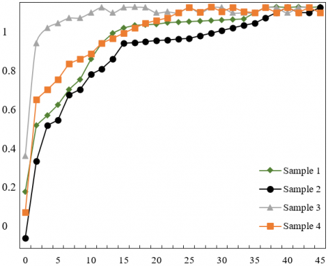
Figure 4 shows the rehabilitation stages of the patients classified based on the fusion feature extraction results on plantar pressure images. Our algorithm achieved relatively good recognition performance on different patient samples, and the recognition accuracy remained stable. With the growing number of samples, the recognition rate of each stage reached the ideal state, and the missing rate was far smaller than 0.05. Table 1 presents the experimental results on different patients in different rehabilitation stages.
For each plantar pressure image sample, this paper firstly extracts the low-frequency components through wavelet transform, then corrects the pixels of the extracted components, and finally extracts the direction features with the HOG descriptor. The accuracy of our method in extracting fusion features was compared with HOG algorithm, wavelet transform algorithm, and principal component analysis (PCA) algorithm (Figure 5). The comparison shows that our fusion feature extraction algorithm achieved the best extraction effect.
Figure 4. Rehabilitation stage classification based on fusion feature extraction
Figure 5. Comparison of feature extraction accuracies
Table 1. Experimental results on different patients in different rehabilitation stage
|
Subset number |
Early rehabilitation stage |
Mid rehabilitation stage |
Late rehabilitation stage |
Full rehabilitation stage |
|
|
Sample 1 |
Single |
86.25 |
85.16 |
97.28 |
86.15 |
|
Fusion |
97.16 |
96.38 |
97.42 |
91.28 |
|
|
Sample 2 |
Single |
88.16 |
87.38 |
82.48 |
85.16 |
|
Fusion |
97.61 |
98.35 |
95.62 |
95.27 |
|
|
Sample 3 |
Single |
89.12 |
89.11 |
87.28 |
88.16 |
|
Fusion |
98.27 |
96.18 |
95.28 |
98.16 |
|
|
Sample 4 |
Single |
85.66 |
89.44 |
87.66 |
85.36 |
|
Fusion |
95.11 |
95.34 |
96.49 |
96.74 |
|
Table 2. Measured results and measuring errors of foot laceration patients
|
Parameter number |
1 |
2 |
3 |
4 |
5 |
6 |
7 |
8 |
9 |
10 |
|
Actual value (cm) |
25.1 |
25.6 |
24.3 |
26.1 |
23.6 |
25.4 |
24.2 |
25.4 |
23.8 |
25.0 |
|
Measured value (cm) |
25.26 |
25.74 |
23.15 |
25.81 |
23.48 |
25.81 |
23.82 |
25.29 |
23.48 |
25.24 |
|
Absolute error (cm) |
0.15 |
0.41 |
0.27 |
0.11 |
0.22 |
0.17 |
0.32 |
0.14 |
0.25 |
0.18 |
|
Relative error (%) |
0.54 |
5.12 |
6.74 |
3 |
2.84 |
5.19 |
4.26 |
1.14 |
3.29 |
4.72 |
|
Parameter number |
11 |
12 |
13 |
14 |
15 |
16 |
17 |
18 |
19 |
20 |
|
Actual value (cm) |
6.2 |
6.3 |
6.7 |
6.7 |
5.5 |
5.4 |
17.2 |
15.4 |
15.6 |
13.7 |
|
Measured value (cm) |
6.32 |
6.22 |
6.69 |
6.51 |
5.6 |
5.6 |
19.24 |
15.16 |
16.82 |
13.72 |
|
Absolute error (cm) |
0.07 |
0.37 |
0.33 |
0.2 |
0.39 |
0.07 |
0.62 |
0.52 |
0.85 |
0.14 |
|
Relative error (%) |
2.9 |
0.72 |
5.62 |
5.17 |
1.28 |
3 |
0.45 |
4.59 |
6.3 |
0.28% |
Figure 6. Sketch map of our measuring method for plantar pressure
Figure 6 illustrates our measuring method for plantar pressure. Considering the characteristics of the proposed fusion feature extraction algorithm, 20 foot shape features were extracted from the plantar pressure images of both feet, including length, width, key point spacing, and pressure areas, the distance from each toe in each foot to the most protruding point at the back of the heel, the widths of the front foot, mid foot, and rear foot, the total plantar area, and the pressure area. Table 2 shows the measured results and measuring errors of foot laceration patients.
This paper mainly investigates the image feature analysis and dynamic measurement of plantar pressure based on fusion feature extraction. After explaining the ideas of extracting image features by combining wavelet transform and HOG descriptor, the authors computed the plantar parameters based on plantar pressure images, and detailed the measurement steps of plantar parameters. Then, experiments were carried out to obtain the plantar pressure waveforms in different rehabilitation stages. Besides, the rehabilitation stages of the patients were classified based on the fusion feature extraction results, and the experimental results on different patients were obtained in different rehabilitation stages. The results show that our algorithm achieved relatively good recognition performance on different patient samples, and the recognition accuracy remained stable. In addition, the feature extraction accuracy of our fusion feature extraction algorithm was compared with that of HOG algorithm, wavelet transform algorithm, and PCA algorithm. The comparison shows that our fusion feature extraction algorithm achieved the best extraction effect. Finally, the measured results and measuring errors of foot laceration patients were given, which demonstrate the effectiveness of our plantar parameter measurement method.
This work was supported by the Project of Changchun Bureau of Science and Technology, Project Name: Rehabilitation massage system based on the output of the standard mechanical evaluation technique (Grant No.: 21ZGM31). By the project of Jilin Provincial National Development and Reform Commission in 2020 (Grant No.: 2020C031-2). Project Name: Research on multi-modal rehabilitation training system of upper limb Motor Function based on Finite state machine Model. By the Innovation Team Project of Jilin Provincial Department of Science and Technology in 2021 Project Name: Research and Development of Intelligent Pressure Ulcer Prevention System. By the project of Jilin Provincial Bureau of Science and Technology (Grant No.: 212558JC010686261), Project Name: Standard acupoint calibration based on machine vision in the intelligent rehabilitation massage system.
[1] Kumar, V.D., Malathi, S., Kumar, V.D., Kannan, P. (2015). Performance improvement using an automation system for segmentation of multiple parametric features based on human footprint. Journal of Electrical Engineering and Technology, 10(4): 1815-1821. https://doi.org/10.5370/JEET.2015.10.4.1815
[2] Ling, J.Y., He, X., Wei, Z.H., Li, Y.M., Liang, G.L. (2014). Footprint automatic alignment algorithm fusing texture features and depth information. Optics And Precision Engineering, 22(7): 1946-1954. https://doi.org/10.3788/OPE.20142207.1946
[3] Askari, Z., Esmaeili, H. (2021). Effect of trunk muscles fatigue on plantar pressure distribution in novice runners. Journal of Biomechanics, 122: 110487. https://doi.org/10.1016/j.jbiomech.2021.110487
[4] Cao, Z., Wang, F., He, Y., Zhang, Y., Zhang, J. (2021). Analysis of plantar pressure in elderly diabetic patients with peripheral neuropathy. 2021 International Conference on Public Health and Data Science (ICPHDS), Chengdu, China, pp. 184-187. https://doi.org/10.1109/ICPHDS53608.2021.00044
[5] Horng, J., Liu, X.C., Thometz, J., Tassone, C., Duey-Holtz, A. (2021). Evaluation of plantar pressures and center of pressure trajectories in Adolescent Idiopathic Scoliosis. Studies in Health Technology and Informatics, 280: 131-135. https://doi.org/10.3233/shti210451
[6] Jiang, X.Y., Li, S.D., Teo, E.C., Zhou, Z.X. (2021). The effect of high-intensity intermittent training on the acute gait plantar pressure in healthy young adults. Journal of Biomimetics, Biomaterials and Biomedical Engineering, 49: 21-32. https://doi.org/10.4028/www.scientific.net/JBBBE.49.21
[7] Castro, M., Abreu, S., Sousa, H., Machado, L., Santos, R., Vilas-Boas, J.P. (2013). Ground reaction forces and plantar pressure distribution during occasional loaded gait. Applied Ergonomics, 44(3): 503-509. https://doi.org/10.1016/j.apergo.2012.10.016
[8] Lin, Y.C., Lin, Y.T. (2013). Human recognition based on plantar pressure patterns during gait. Journal of Mechanics in Medicine and Biology, 13(2): 1350039. https://doi.org/10.1142/S0219519413500395
[9] Chockalingam, N., Healy, A., Naemi, R., Burgess-Walker, P., Razak, A.H.A., Zayegh, A., Wahab, Y. (2013). Comments and reply to: Foot plantar pressure measurement system: A review. Sensors 2012, 12, 9884-9912. Sensors, 13(3): 3527-3529. https://doi.org/10.3390/s130303527
[10] Zhou, J., Li, T., Xu, B., Chen, W. (2015). Investigation of children's plantar pressure distribution with varied angle of hallux. Revista de Pielarie Incaltaminte, 15(1): 3-14.
[11] D'Août, K., Stassijns, G., Aerts, P., Willems, C. (2015). Plantar pressure and foot roll-off timing during walking barefoot, in a minimal shoe, and in conventional footwear. Footwear Science, 7(S1): S119-S120. https://doi.org/10.1080/19424280.2015.1038641
[12] Li, T., Li, B., Chen, W., Wu, J., Xu, B., Zhou, J. (2015). Reliability analysis of footscan plate system in measurement of plantar pressure of spastic diplegia children. Revista de Pielarie Incaltaminte, 15(4): 239-248.
[13] Chen, W.M., Lee, S.J., Lee, P.V.S. (2015). Plantar pressure relief under the metatarsal heads–Therapeutic insole design using three-dimensional finite element model of the foot. Journal of Biomechanics, 48(4): 659-665. https://doi.org/10.1016/j.jbiomech.2014.12.043
[14] Jafarzadeh, E., Soheilifard, R., Ehsani-Seresht, A. (2021). Design optimization procedure for an orthopedic insole having a continuously variable stiffness/shape to reduce the plantar pressure in the foot of a diabetic patient. Medical Engineering & Physics, 98: 44-49. https://doi.org/10.1016/j.medengphy.2021.10.008
[15] Wafai, L., Zayegh, A., Woulfe, J., Aziz, S.M., Begg, R. (2015). Identification of foot pathologies based on plantar pressure asymmetry. Sensors, 15(8): 20392-20408. https://doi.org/10.3390/s150820392
[16] Wang, D., Li, Z., Dey, N., Ashour, A.S., Moraru, L., Biswas, A., Shi, F. (2019). Optical pressure sensors based plantar image segmenting using an improved fully convolutional network. Optik, 179: 99-114. https://doi.org/10.1016/j.ijleo.2018.10.155
[17] Li, Z. (2019). Region based extraction of plantar pressure images with R-CNN and fast R-CNN. Information Technology and Intelligent Transportation Systems, 314: 362-368. https://doi.org/10.3233/978-1-61499-939-3-362
[18] Tafti, N., Turk, S.B., Hemmati, F., Norouzi, E., Sharifmoradi, K., Karimi, M.T., Kashani, R.V. (2019). Effect of wearing insole with different density on standing and walking plantar pressure distribution. Journal of Mechanics in Medicine and Biology, 19(3): 1950006. https://doi.org/10.1142/S0219519419500064
[19] Zhang, C., Pan, S., Qi, Y., Yang, Y. (2019). A footprint extraction and recognition algorithm based on plantar pressure. Traitement du Signal, 36(5): 419-424. https://doi.org/10.18280/ts.360506
[20] Wang, C., Li, D., Li, Z., Wang, D., Dey, N., Biswas, A., Shi, F. (2019). An efficient local binary pattern based plantar pressure optical sensor image classification using convolutional neural networks. Optik, 185: 543-557. https://doi.org/10.1016/j.ijleo.2019.02.109
[21] Sabry, A.H., Sabry, A., Hasan, W.Z.W., Mohtar, M.N., Ahmad, R.M.K.R., Ramli, H.R., Hamid, Z.H.A. (2018). Foot plantar pressure distribution modeling based on image processing. 2018 IEEE 5th International Conference on Smart Instrumentation, Measurement and Application (ICSIMA), Songkhla, Thailand, pp. 1-4. https://doi.org/10.1109/ICSIMA.2018.8688776