Ali Arshaghi | Mohsen Ashourin* | Leila Ghabeli
© 2021 IIETA. This article is published by IIETA and is licensed under the CC BY 4.0 license (http://creativecommons.org/licenses/by/4.0/).
OPEN ACCESS
Using machine vision and image processing as a non-destructive and rapid method can play an important role in examining defects of agricultural products, especially potatoes. In this paper, we propose a convolution neural network (CNN) to classify the diseased potato into five classes based on their surface image. We trained and tested the developed CNN using a database of 5000 potato images. We compared the results of potato defect classification based on CNN with the traditional neural network and Support Vector Machine (SVM). The results show that the accuracy of the deep learning method is higher than the Traditional Method. We get 100% and 99% accuracy in some of the classes, respectively.
convolutional neural networks, deep learning, defect detection, potato diseases
Machine vision is one of the most widely used technologies in modern food and agricultural industries. This technology is a cost-effective tool for the rapid and accurate evaluation of food quality. The determination of surface defects of potatoes is important in automatic defect detection. The potato plant hosts many pathogens, including bacteria, fungus, viroids, viruses, and phytoplasmas. These pathogens can reduce product yield and quality individually or together. Adverse environmental conditions and some specific crop conditions can also have adversely affected the potato plant health and product quality. Control of pathogens and avoidance of aggravating conditions is one of the important goals of commercial potato production centers.
Several image processing methods have been reported for potato diseases detections. Al Riza et al. [1] used diffuse reflection features to detect potato surface defects. Su et al. [2] presented a three-dimensional approach for identifying and predicting the characteristics of a potato-based on machine vision. In this study, a three-dimensional surface model of potatoes that uses two images is developed. The model is very accurate in calculating potato volume. Using a depth and color camera, they extracted potato surface information like length, width, thickness, area, volume and two-dimensional border changes. The success rate in potato size grading with the volume density model reaches 93%, while with the area concentration model it reaches 73%.
Gao et al. [3] diagnosed damaged skin (Solanum tuberosum L problem) in potato tubers by comparing the visible and biospeckle imaging. They extracted properties like pixel color and texture characteristics of surface potato from the image surface. Least-squares SVM, and binary logistic regression (BLR) is used for classification. Their best maximum classification accuracy is 90%.
Brar and Singh performed a C-mean fuzzy clustering for segmentation in this potato defect detection [4]. The proposed scheme has 95% accuracy in grading the potatoes in three basic external faults, including greening, spoiled, rotten, and potato slits [4]. All three types are 100% are identified. However, some healthy images incorrectly identified as defective, using of fuzzy c-mean clustering is very effective in segmenting potato images into healthy and defective areas [4].
Moallem et al. [5] suggested color image segmentation of the potato using an inference fuzzy system. The accuracy of the proposed algorithm segmentation rate is 98% on 500 potato images. They used HSV color space, genetic algorithm thresholding, and morphology to detect the defected segment. In another research, Moallem et al. performed potato defect using neural network and support vector machine [6]. After preprocessing and features extracting stage, classification methods including ANN and SVM, are used to identify the potato diseases. The results show that the SVM classifier has better performance than the radial bases function (RBF) and multilayer perceptron (MLP) neural networks on the detection of potato defects [6]. The correct detection rate (CDR) for SVM is about 96.7%. Their method showed the defective part of the potato [6]. In another paper, Razmjooy and Daviran [7] reported potato defect detection using machine vision and neural networks. After the segmentation and feature extraction stage, classification methods such as MLP, SVM, RBF are used to identify the potato problems. The results show that the SVM classifier has better performance. Based on tests on different input images, it is shown that the SVM method has high accuracy and high value compared to MLP and RBF. The accuracy is over 90% percent. Razmjooy et al. [8] after pre-processing with classification methods such as MLP, SVM, KNN methods, identified the faulty part of the potato. The results show that the SVM classifier has high speed and accuracy among classifiers for defect detection. It has 95% accuracy in classification and 96.86% accuracy in classification.
Deep learning has been widely used in recent years such as in the large-scale image recognition, for remote sensing, architectures, predicting the sequence specificities of DNA- and RNA-binding proteins, detecting robotic grasps, visual understanding, in processing images, video, speech and audio, [9-19]. Deep learning also accurately detects crop diseases in agriculture and its accuracy is more than previous and traditional methods [10-12].
We are examining two goals in this paper. CNN parameters and structure are improved to classify and recognize different classes of the potato images. We also simulate some traditional intelligent system for potato classification and compare their results with the CNN based method. The diseases we detect are Gray Mold, Skin Spot, Common Scab, Gangrene and Leak. The classification of 5 classes in this article is a new task for diagnosing surface defects of potatoes, and the previous researches classified them into two groups of healthy and defective. The results show that the accuracy of the deep learning method is higher than the traditional method, and get 100% and 99% accuracy in some of the classes.
This remaining part of the paper is as follow. In Section I, we express the introduction of surface defect potato and study research in this field. In Section II, we explain the proposed methods, and in section III simulation results of two methods are presented and compared with other traditional methods for surface defect potato. Finally, the last section is conclusion.
2.1 Dataset
We provide 5000 potato images. All images were taken from databases CFIA, USDA and potatoes farms in Ardebil, the city of Iran. Dataset images had all major types of potato diseases. All the input images have the same size.
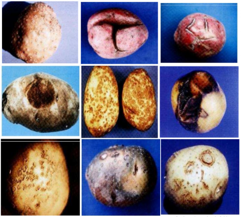
Several types of potato diseases are shown in Figure 1. Several of potato diseases have been studied in this study, names of potato diseases are Bacterial Ring Rot, Clostridium spp, Common Scab, Gangrene, Rosellinia Black Rot, Gray Mold, Septoria Leaf Spot, Silver Scurf, Skin Spot and Leak.
Our system classifies the potatoes to 5 types, one is healthy and the others are Leak, Gangrene, Gray Mold, Skin Spot and Common Scab.
Data gathering and training are essential for CNNs. More learned data yield more accurate classification. For CNN training a lot of data needs to be acquired, and the current potato images collected are not enough. We increase the data set in various ways, including rotating the image to 90°, 180°, 270°, cropping center of the image and transforming to grayscale. Increasing the number of datasets helps to reduce overfitting during training. We use 80% of data for training and 20% for testing.
Figure 1. Nine common potato diseases
2.2 Image preprocessing and labelling
To implement better feature extraction, the images in the dataset are pre-processed. It is important to normalize the image size. In this study, all images were resized to 32 x 32 by MATLAB software. All classes in the dataset and the training and testing set are separated.
2.3 Convolutional Neural Networks
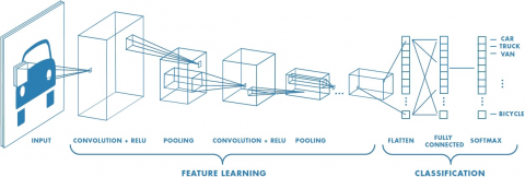
Figure 1 shows an architecture of the convolutional neural network to classify [20]. An overview of convolutional neural network architecture is displayed in Figure 2. There are two steps to train this method, the feed-forward phase and the backpropagation phase. The network training ends after repeating suitable numbers of these steps.
The convolutional neural network uses layers such as: pooling layer, fully connected layers.
In Figure 3 you can see the Max pooling process [20, 21]. In the fully connected layer the result network is shown in vector and we can use it for images classification [22] or for subsequent processing [23].
There are some popular models for CNN used in researches. These methods are AlexNet [20], the Visual Geometry Group (VGG) [24], GoogleNet [25] and Inception-ResNet [26]. Each model has different performance and advantages [27]. This models and networks trained through some data set to perform recognition for problems [28, 29].
Some research works applied CNN architectures ResNetA, lexNet, and VGG, and some researchers used the CNN with PCA [30], SVM [31], macroscopic cellular automata [32], linear regression [33], large margin classifiers (LMC) [34]. Some papers used the popular architecture DL framework with Caffe, Theano, Pylearn2, MatConvNet, and Deep Learning Matlab Toolbox, Tensor Flow.
Figure 2. An outline of the convolutional neural network architecture
Figure 3. Max pooling step
Some researchers combine CNN architectures to take the advantages [28] and use the popular CNN models knowledge for increasing the learning efficiency and changing pre-trained models. We use another pre-trained model when we don’t have enough training data set. Usually Pre-trained CNN have been trained by proper data set. These models studied and followed by Lee et al. [35], Reyes et al. [36], Sa et al. [37], Steen et al. [38], Bargoti and Underwood [39], Douarre et al. [31], Mohanty et al. [40], Christiansen et al. [38], Lu et al. [41] and Sørensen et al. [42] for the VGG16, DenseNet, AlexNet and GoogleNet architectures.
Deep learning is used extensively in different areas of computer vision like image classification, object detection, semantic segmentation and image retrieval which are key activities to understand the image. In this section we summarize the images categories with deep-learning in crops.
Sample of studied papers in agriculture is state in Table 1.
Table 1. Sample of studied papers in agriculture
|
Product |
Method |
Accuracy |
Year |
Author |
|
potato |
PLS-GA |
97.6% |
2017 |
Dimas |
|
fruit |
SVM,LDA, PCA |
83%, 89% |
2017 |
Jose |
|
tomato |
Wavelet and radon |
94%,91%,89% |
2017 |
Maduguri Sudhir |
|
Classify banana leaf diseases |
deeplearning4j |
90% |
2017 |
Amara et al. |
|
potato |
Fuzzy C-mean |
95% |
2016 |
Er. Amrinder |
|
potato |
LS-SVM (Least Square Support Vector Machine), BLR (Binary Logistic Regression) |
90% |
2016 |
Yingwang Gao |
|
apple |
SVM, MLP, KNN |
96.7% |
2016 |
moallem |
|
pomegranate |
SURF Feature extraction |
89.2%-92.5% |
2016 |
Yogesh |
|
tomato |
Fuzzy logic |
98.6 |
2016 |
Lenard C. Dorado |
|
orange |
PCA |
93% |
2016 |
Jiangbo Li |
|
apple |
fuzzy-C means |
|
2016 |
Hamidreza Saberkari |
|
mango |
SDA,ANN, FD |
|
2016 |
Dameshwari Sahu |
|
apple |
MLP, Fuzzy logic |
- |
2016 |
Misigo Ronald |
|
Classify 91 weed seed types |
PCANet + LMC classifiers |
96% + (CA), 0.968 (F1) |
2015 |
Xinshao and Cheng |
|
potato |
Fuzzy logic, GA |
88.10% |
2014 |
razmjooy |
|
potato |
MLP, SVM, RBF |
95%,96%,86% |
2011 |
razmjoo |
3.1 Simulation with MLP, RBF, and SVM
In this section we simulated traditional methods. We use three classification methods of MLP, RBF, and SVM.
Figure 4. The diagram of developed systems in Section 3.1
3.1.1 Equipment for simulation
Matlab software is applied in all stages. The computer specifications are Memory: 4Gb, Processor: Intel Core i7-7700 CPU @3.60 GHz 3.60 GHz.
3.1.2 The diagram of developed traditional system
Figure 4 shows the diagram of developed traditional systems.
3.1.3 Data sources and Image acquisition
We produce some potato images taken with the camera from the farm and resize them. The number of the dataset in this section is 1000. In this example, we set the size potato to 256x256. Almost 30% of potatoes are healthy and 70% are defective.
3.1.4 Segmentation
Classification is the first step and the most critical stage of the analyzed image, which aims extracting the information within the inner image (edges, fronts, and the identity each of the regions) through described, regions and reducing them to a suitable form for computer processing and diagnostics of the regions. The resulting segmentation will have a significant impact on the accuracy of features evaluation. Segmentation is often a description of the process of dividing the image into main components and extracting interest object. Otsu method is used for segmentation.
3.1.5 Feature extraction
Huang et al. [43] developed a new method using the SIFT algorithm. In this method, first, SIFT descriptors are extracted from the image. The key point of this algorithm is the SIFT descriptors are resistant to changes in scale, rotation, and brightness. Therefore, matching these descriptors can be used to identify duplicated regions. The SIFT algorithm extracts the distinguishing features of local fragment images that are resistant to scaling and rotation. These features are also powerful against changes such as noise, distortion, and brightness, and give the same results.
3.1.6 Classification
In this section, we examine three types of classification approaches, Multi-Layer-Perceptron (MLP), Radial Basis Function Networks (RBF), and Support Vector Machines (SVM), and Simulation results and classification accuracy are shown. We use also some papers in this field such as [44-46].
3.1.7 Implementation parameters
The performance of the MLP method is selected as:
Learning rate= 0.01
Epochs= 1000
Target error goal: 10-4
Radial Basis Function has its maximum, 1 if its input is 0; since to reduce w (weight vector) and p (input), the output is increased. a radial basis neuron produces 1 when the input p is as similar as its weight vector p [47].
In SVM we set End-accuracy: 10-4, we select the input image 256*256 for easily comparing. All of the images converted to this size. The result of experiments, show that RBF networks have higher performance than the MLP. SVM classifier is the best classifier for potato defect detections.
There are three metrics for comparing the performance of applied methods. These metrics are: the correct detection rate (CDR), The false acceptance rate (FAR), the false rejection rate (FRR) [6], which are defined in (1).
$C D R=\frac{\text { Number of samples correctly classified in dataset }}{\text { Total number of samples in dataset }}$
$F A R=\frac{\text { Number of non }-\text { potato samples classified as potato samples }}{\text { Total number of samples in dataset }}$ (1)
$F R R=\frac{\text { Number of potato samples classified as non-potato samples }}{\text { Total number of samples in dataset }}$
3.2 Simulation with CNN
The initial learning rate of the model is 0.0001, top - 5 testing accuracy is 100%. Figure 5 displays the curve of the system loss. the top - 5 identification accuracy converge after 480th iterations and can see that. The training time and the convergence time of the model are long. Learning Rate and Loss and accuracy with each Iteration showed in Table 4. In Epoch 10 and Iteration 480, value accuracy is 100%, and Time Elapsed is accurate too. The model also has very parameters.
Parameter network and structure our deep CNN network are displayed in Table 2. Considering the various tests performed in the article implementation program and comparing similar work done in the articles [48], the size of deep learning layers, parameters setting, several Epochs and number of Relu Layer, convolution2d Layer and Fully Connected Layer and learning rate and the number of iterations and so on. At the end the values of Table 2 are selected to get high classification accuracy.
Table 2. Parameters deep network for this paper
|
Name |
Parameters |
Name |
Parameters |
|
Solver type |
SGD |
'Mini Batch Size' |
100 |
|
Base learning rate |
0.001 to 0.0001 |
convolution2d Layer |
Two layer |
|
'Validation Frequency' |
30 |
Relu Layer |
Two layer |
|
Learning rate |
0.0001 |
Max Pooling2d Layer |
Two layer, 'Stride',2 |
|
Initial Learn Rate |
0.001 |
Fully Connected Layer |
384 class |
|
Learn Rate Schedule |
'piecewise' |
Fully Connected Layer |
192 class |
|
'Learn Rate Drop Factor' |
0.1 |
Fully Connected Layer |
4 class |
|
Hardware resource |
Single CPU |
Softmax Layer |
One layer |
|
iteration |
480 |
Classification Layer |
One layer |
|
'L2Regularization' |
0.004 |
'Learn Rate Drop Period' |
8 |
|
'Max Epochs' |
10 |
|
|
4.1 Results for traditional methods
The number of repeats is 100 times. The mean classification rate was calculated correctly and tested 20 times to obtain statistical comparisons between the SVM, RBF, and MLP methods. In Table 3 we show the performance of each method and its accuracy on databases CFIA [49], USDA [50] and a custom database.
Table 3. Neural networks accuracy in three databases
|
Test Accuracy |
|||
|
Database |
MLP |
RBF |
SVM |
|
USDA |
81% |
83% |
90% |
|
CFIA |
80% |
82% |
89% |
|
Custom |
86% |
87% |
91% |
4.2 Result for CNN method
4.2.1 Test on the sample from group one
Figure 5(a) displays the changes accuracy and system loss than to iterations. Learning Rate and Loss and accuracy with each Iteration showed in Table 4. In the Epoch 10 and Iteration 480, value accuracy is 100%. The following Figure 6 is an example of a test performed to detect the first class of potato surface defects from the data set which classification accuracy is 100% for this first class.
CNN Accuracy in first class is 100% and in the others class accuracy are 0%. Therefore, this potato image is in first class.
Table 4. Learning rate and loss and accuracy with each iteration for group one
|
Epoch |
Iteration |
Time Elapsed (hh:mm:ss) |
Mini-batch Accuracy |
Mini-batch Loss |
Base Learning Rate |
|
1 |
1 |
00:00:08 |
20.00% |
1.6078 |
0.0010 |
|
2 |
50 |
00:03:52 |
34.00% |
1.4722 |
0.0010 |
|
3 |
100 |
00:07:16 |
51.00% |
1.1939 |
0.0010 |
|
4 |
150 |
00:10:41 |
81.00% |
0.6212 |
0.0010 |
|
5 |
200 |
00:14:06 |
87.00% |
0.3554 |
0.0010 |
|
6 |
250 |
00:17:25 |
93.00% |
0.1806 |
0.0010 |
|
7 |
300 |
00:20:43 |
88.00% |
0.2063 |
0.0010 |
|
8 |
350 |
00:24:03 |
98.00% |
0.1133 |
0.0010 |
|
9 |
400 |
00:27:21 |
94.00% |
0.1474 |
0.0001 |
|
10 |
450 |
00:30:39 |
100.00% |
0.0254 |
0.0001 |
|
10 |
480 |
00:32:39 |
100.00% |
0.0250 |
0.0001 |
Figure 5. The curve of the system loss for group one
Figure 6. Variation of partial accuracy based on iterations for group one
4.2.2 Test on the sample from group second
Figure 7 displays the changes of accuracy and system loss versus iterations. Learning Rate, Loss and accuracy with each Iteration are shown in Table 5. In Epoch 10 and Iteration 480, value accuracy is 98%. The following Figure 8 is an example of a test performed to detect the second class of potato surface defects from the data set for which classification accuracy is 98% for this second class.
CNN Accuracy in second class is 98% and in the One class accuracy is 2%. Therefore, this potato image is in the second class.
Figure 7. The curve of the system loss for group 2
Figure 8. Variation of partial accuracy based on iterations for group 2
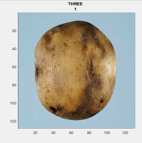
4.2.3 Test on the sample from group third
Figure 9 displays the changes of accuracy and system loss versus iterations. Learning Rate, Loss and accuracy with each Iteration are shown in Table 5. In the Epoch 10 and Iteration 480, value accuracy is 100%. The following Figure 10 is an example of a test performed to detect the third class of potato surface defects from the data set which classification accuracy is 100% for this third class.
CNN Accuracy in third class is 100% and in the others class accuracy are 0%. Therefore, this potato image is in third class.
Figure 9. Variation of loss based on iterations for group 3
Figure 10. Variation of partial accuracy based on iterations for group 3
4.2.4 Test on the sample from group Fourth
Figure 11 displays the changes of accuracy and system loss versus iterations. Learning Rate, Loss and accuracy with each Iteration are shown in Table 5. In Epoch 10 and Iteration 480, value accuracy is 99%. The following Figure 12 is an example of a test performed to detect the Forth class of potato surface defects from the data set which classification accuracy is 99% for this Forth class.
CNN Accuracy in forth class is 99% and in the third class accuracy is 0.5%, and in the fifth class accuracy is 0.5%. Therefore, this potato image is in the fourth class.
Figure 11. Variation of loss based on iterations for group 3
Figure 12. Variation of partial accuracy based on iterations for group 4
4.2.5 Test on the sample from group Fifth
Figure 13 displays the changes of accuracy and system loss versus iterations. Learning Rate, Loss and accuracy with each Iteration are shown in Table 5. In the Epoch 10 and Iteration 480, value accuracy is 100%. The following Figure 14 is an example of a test performed to detect the Fifth class of potato surface defects from the data set for which classification accuracy is 100% for this Fifth class.
CNN Accuracy in fifth class is 100%, and in the others class accuracy are 0%. Therefore, this potato image is in fifth class.
Figure 15 displays the accuracy of each class according to the iteration number.
Figure 13. Variation of loss based on iterations for group 5
Figure 14. Variation of partial accuracy based on iterations for group 5
Table 5. Learning rate and loss and accuracy with each Iteration for all group
|
Epoch |
Iteration |
Time Elapsed (hh:mm:ss) |
Mini-batch Accuracy |
Mini-batch Loss |
Base Learning Rate |
class |
|
10 |
480 |
00:32:39 |
100.00% |
0.0250 |
0.0001 |
one |
|
10 |
480 |
00:33:22 |
98.00% |
0.0503 |
0.0001 |
second |
|
10 |
480 |
00:33:56 |
100.00% |
0.0065 |
0.0001 |
third |
|
10 |
480 |
00:34:24 |
99.60% |
0.0517 |
0.0001 |
forth |
|
10 |
480 |
00:31:41 |
100.00% |
0.4659 |
0.0001 |
fifth |
Figure 15. The accuracy of each class according to the iteration number
Figure 16 shows the confusion matrix for the CNN network. Each cell in the confusion matrix defined the percentage of images of the row’s class that were categorized into the column’s class of diseases potato. The results show that 100% Gray Mold and Skin Spot disease potato were classified, and 95.34% Common Scab disease potato were classified. The percentage portion of each of the row classes in the column classes is shown, for example in the first row of Common Scab, 95.34% is for Common Scab disease potato, and 3.64 this disease is for Gray Mold disease potato, and 1.02 is for Gangrene disease potato.
Figure 16. The confusion matrix of the CNN model rows are the actual classes of an image. Columns are CNN’s class prediction
We examine the CNN performance for different usage of available data for improve the classification and decrease the error rate must use the more data from the data set. Table 6 shows the accuracy for different exams.
Table 6. CNN model accuracy in each train–test set
|
Train-Test set split |
Accuracy |
|
|
Portion |
Number |
|
|
90%-10% |
4331-481 |
98.65% |
|
80%-20% |
3850-962 |
98.32% |
|
70%-30% |
3369-1443 |
97.59% |
|
60%-40% |
2887-1925 |
97.43% |
|
50%-50% |
2406-2406 |
95.64% |
|
40%-60% |
1925-2887 |
94.37% |
|
30%-70% |
1443-3369 |
93.23% |
|
20%-80% |
962-3850 |
90.04% |
|
10%-90% |
481-4331 |
87.56% |
In this paper, we examined the detection and classification of surface potato defects using image processing and neural network, RBF, MLP, and SVM, and CNN. In the traditional intelligent methods, we simulate and report the performances of each method and its accuracy on databases CFIA, USDA, and a custom database. SVM classifier is the best classifier for potato defect detections. By using our deep CNN network displayed in Table 2, we get high classification accuracy. The CNN based method has higher accuracy than other techniques. In our paper, we achieved 100% and 99% accuracy in surface potato defects categorization. Some potato diseases are well categorized which the confusion matrix shows it. Potato diseases potato are Gray Mold, Skin Spot, Common Scab, Gangrene and Leak. The classification of 5 classes in this article is a new task for diagnosing surface defects of potatoes, and the previous researches classified them into two groups of healthy and defective. The number of images used in the potato dataset is 5000, and this high accuracy indicates the success of the method used.
[1] Al Riza, D.F., Suzuki, T., Ogawa, Y., Kondo, N. (2017). Diffuse reflectance characteristic of potato surface for external defects discrimination. Postharvest Biology and Technology, 133: 12-19. https://doi.org/10.1016/j.postharvbio.2017.07.006
[2] Su, Q., Kondo, N., Li, M., Sun, H., Al Riza, D.F. (2017). Potato feature prediction based on machine vision and 3D model rebuilding. Computers and Electronics in Agriculture, 137: 41-51. https://doi.org/10.1016/j.compag.2017.03.020
[3] Gao, Y., Geng, J., Rao, X., Ying, Y. (2016). CCD-based skinning injury recognition on potato tubers (Solanum tuberosum L.): A comparison between visible and biospeckle imaging. Sensors, 16(10): 1734. https://doi.org/10.3390/s16101734
[4] Brar, E.A.S., Singh, K. (2016). Potato defect detection using fuzzy c-mean clustering based segmentation. Indian Journal of Science and Technology, 9(32): 1-6. https://doi.org/10.17485/ijst/2016/v9i32/100737
[5] Moallem, P., Razmjooy, N., Mousavi, B.S. (2014). Robust potato color image segmentation using adaptive fuzzy inference system. Iranian Journal of Fuzzy Systems, 11(6): 47-65. https://doi.org/10.22111/IJFS.2014.1748
[6] Moallem, P., Razmjooy, N., Ashourian, M. (2013). Computer vision-based potato defect detection using neural networks and support vector machine. International Journal of Robotics and Automation, 28(2): 137-145. https://doi.org/10.2316/Journal.206.2013.2.206-3746
[7] Razmjooy, N., Daviran, R. (2011). Potato defect detection using computer vision and neural networks. Majlesi Conference on Electrical Engineering.
[8] Razmjooy, N., Mousavi, B.S., Soleymani, F. (2012). A real-time mathematical computer method for potato inspection using machine vision. Computers & Mathematics with Applications, 63(1): 268-279. https://doi.org/10.1016/j.camwa.2011.11.019
[9] Lecun, Y., Bengio, Y. Hinton, G. (2015). Deep learning. Nature, 521: 436-444. https://doi.org/10.1038/nature14539
[10] Guo, Y., Liu, Y., Oerlemans, A., Lao, S., Wu, S., Lew, M.S. (2016). Deep learning for visual understanding: A review. Neurocomputing, 187: 27-48. https://doi.org/10.1016/j.neucom.2015.09.116
[11] Lenz, I., Lee, H., Saxena, A. (2013). Deep learning for detecting robotic grasps. International Journal of Robotics Research, 34: 705-724. https://doi.org/10.1177/0278364914549607
[12] Alipanahi, B., Delong, A., Weirauch, M.T., Frey, B.J. (2015). Predicting the sequence specificities of DNA- and RNA-binding proteins by deep learning. Nature Biotechnology, 33: 831-838. https://doi.org/10.1038/nbt.3300
[13] Zhang, L.P., Xia, G.S., Wu, T.F., Lin, L., Tai, X.C. (2015). Deep learning for remote sensing image understanding. Journal of Sensors, 2016: 12-13. https://doi.org/10.1155/2016/7954154
[14] Bengio, Y. (2009). Learning deep architectures for AI. Foundations & Trends® in Machine Learning, 2: 1-127. https://doi.org/10.1561/2200000006
[15] Everingham, M., Van Gool, L., Williams, C.K., Winn, J., Zisserman, A. (2010). The pascal visual object classes (VOC) challenge. International Journal of Computer Vision, 88(2): 303-338. https://doi.org/10.1007/s11263-009-0275-4
[16] Russakovsky, O., Deng, J., Su, H., Krause, J., Satheesh, S., Ma, S., Huang, Z., Karpathy, A., Khosla, A., Bernstein, M., Berg, A.C., Li, F.F. (2015). ImageNet large scale visual recognition challenge. International Journal of Computer Vision, 115: 211-252. https://doi.org/10.1007/s11263-015-0816-y
[17] Krizhevsky, A., Sutskever, I., Hinton, G. (2012). ImageNet classification with deep convolutional neural networks. in International Conference on Neural Information Processing Systems (NIPS'12), Lake Tahoe, Nevada USA, 60(6): 1097-1105. https://doi.org/10.1145/3065386
[18] Simonyan, K., Zisserman, A. (2014). Very deep convolutional networks for large-scale image recognition. arXiv preprint arXiv:1409.1556. https://arxiv.org/abs/1409.1556.
[19] Zeiler, M.D., Fergus, R. (2015). Visualizing and understanding convolutional networks. Computer Vision – ECCV 2014. ECCV 2014. Lecture Notes in Computer Science, Springer, Cham, 8689: 818-833. https://doi.org/10.1007/978-3-319-10590-1_53
[20] Krizhevsky, A., Sutskever, I., Hinton, G.E. (2012). Imagenet classification with deep convolutional neural networks. Communications of the ACM, 60(6): 84-90. https://doi.org/10.1145/3065386
[21] Cireşan, D.C., Meier, U., Masci, J., Gambardella, L.M., Schmidhuber, J. (2011). High-performance neural networks for visual object classification. arXiv preprint arXiv:1102.0183. https://arxiv.org/abs/1102.0183.
[22] He, K., Zhang, X., Ren, S., Sun, J. (2015). Spatial pyramid pooling in deep convolutional networks for visual recognition. IEEE Transactions on Pattern Analysis and Machine Intelligence, 37(9): 1904-1916. https://doi.org/10.1109/TPAMI.2015.2389824
[23] Girshick, R., Donahue, J., Darrell, T., Malik, J. (2014). Rich feature hierarchies for accurate object detection and semantic segmentation. The IEEE Conference on Computer Vision and Pattern Recognition (CVPR), PP. 580-587. https://doi.org/10.1109/CVPR.2014.81
[24] Simonyan, K., Zisserman, A. (2014). Very deep convolutional networks for large-scale image recognition. arXiv:1409.1556. https://arxiv.org/abs/1409.1556.
[25] Szegedy, C., Liu, W., Jia, Y., Sermanet, P., Reed, S., Anguelov, D., Erhan, D., Vanhoucke, V., Rabinovich, A. (2015). Going deeper with convolutions. In Proceedings of the IEEE Conference on Computer Vision and Pattern Recognition, pp. 1-9. https://doi.org/10.1109/CVPR.2015.7298594
[26] Szegedy, C., Ioffe, S., Vanhoucke, V., Alemi, A. (2017). Inception-v4, Inception-ResNet and the impact of residual connections on learning. In Proceedings of the Thirty-First AAAI Conference on Artificial Intelligence (AAAI-17). Palo Alto, CA, USA: AAAI, pp. 4278-4284.
[27] Canziani, A., Paszke, A., Culurciello, E. (2016). An analysis of deep neural network models for practical applications. arXiv:1605.07678. https://arxiv.org/abs/1605.07678.
[28] Pan, S.J., Yang, Q. (2010). A survey on transfer learning. IEEE Transactions on Knowledge and Data Engineering, 22(10): 1345-1359. https://doi.org/10.1109/TKDE.2009.191
[29] Deng, J., Dong, W., Socher, R., Li, L.J., Li, K. Li, F.F. (2009). Imagenet: A large-scale hierarchical image database. 2009 IEEE Conference on Computer Vision and Pattern Recognition (CVPR). Miami, FL, USA: IEEE, pp. 248-255. https://doi.org/10.1109/CVPR.2009.5206848
[30] Chen, Y., Lin, Z., Zhao, X., Wang, G., Gu, Y. (2014). Deep learning-based classification of hyperspectral data. IEEE Journal of Selected Topics in Applied Earth Observations and Remote Sensing, 7(6): 2094-2107. https://doi.org/10.1109/JSTARS.2014.2329330
[31] Douarre, C., Schielein, R., Frindel, C., Gerth, S., Rousseau, D. (2016). Deep learning based root-soil segmentation from X-ray tomography. bioRxiv, 071662. https://doi.org/10.1101/071662
[32] Song, X., Zhang, G., Liu, F., Li, D., Zhao, Y., Yang, J. (2016). Modeling spatiotemporal distribution of soil moisture by deep learning-based cellular automata model. Journal of Arid Land, 8(5): 734-748. https://doi.org/10.1007/s40333-016-0049-0
[33] Chen, S.W., Shivakumar, S.S., Dcunha, S., Das, J., Okon, E., Qu, C., Taylor, C.J., Kumar, V. (2017). Counting apples and oranges with deep learning: A datadriven approach. IEEE Robotics and Automation Letters, 2(2): 781-788. https://doi.org/10.1109/LRA.2017.2651944
[34] Wang, X.S., Cai, C. (2015). Weed seeds classification based on PCANet deep learning baseline. 2015 Asia-Pacific Signal and Information Processing Association Annual Summit and Conference (APSIPA), Hong Kong, China, pp. 408-415. https://doi.org/10.1109/APSIPA.2015.7415304
[35] Lee, S.H., Chan, C.S., Wilkin, P., Remagnino, P. (2015). Deep-plant: Plant identification with convolutional neural networks. In 2015 IEEE International Conference on Image Processing (ICIP). Piscataway, NJ, USA, pp. 452-456. https://doi.org/10.1109/ICIP.2015.7350839
[36] Reyes, A.K., Caicedo, J.C., Camargo, J.E. (2015). Fine-tuning deep convolutional networks for plant recognition. CLEF2015 Working Notes. Working Notes of CLEF 2015 – Conference and Labs of the Evaluation Forum, Toulouse, France, Toulouse: CLEF.
[37] Sa, I., Ge, Z., Dayoub, F., Upcroft, B., Perez, T., McCool, C. (2016). Deepfruits: A fruit detection system using deep neural networks. Sensors, 16(8): 1222. https://doi.org/10.3390/s16081222
[38] Steen, K.A., Christiansen, P., Karstoft, H., Jørgensen, R.N. (2016). Using deep learning to challenge safety standard for highly autonomous machines in agriculture. Journal of Imaging, 2(1): 6. https://doi.org/10.3390/jimaging2010006
[39] Bargoti, S., Underwood, J. (2017). Deep fruit detection in orchards. In 2017 IEEE International Conference on Robotics and Automation (ICRA), Singapore, pp. 3626-3633. https://doi.org/10.1109/ICRA.2017.7989417
[40] Mohanty, S.P., Hughes, D.P., Salathé, M. (2016). Using deep learning for image-based plant disease detection. Frontiers in Plant Science, 7: 1419. https://doi.org/10.1109/ICRA.2017.7989417
[41] Lu, H., Fu, X., Liu, C., Li, L.G., He, Y.X., Li, N.W. (2017). Cultivated land information extraction in UAV imagery based on deep convolutional neural network and transfer learning. Journal of Mountain Science, 14(4): 731-741. https://doi.org/10.1007/s11629-016-3950-2
[42] Sørensen, R.A., Rasmussen, J., Nielsen, J., Jørgensen, R.N. (2017). Thistle detection using convolutional neural networks. Montpellier, France: EFITA WCCA 2017 Conference.
[43] Huang, D.S., Wang, X.N., Qin, Q. (2016). An improved SIFT algorithm based on canny operator and Hillbert - Huang transform. Proceedings of the International Conference on Communication and Electronic Information Engineering (CEIE 2016). https://doi.org/10.2991/ceie-16.2017.22
[44] Rani, B.M.S., Majety, V.D., Pittala, C.S., Vijay, V., Sandeep, K.S., Kiran, S. (2021). Road identification through efficient edge segmentation based on morphological operations. Traitement du Signal, 38(5): 1503-1508. https://doi.org/10.18280/ts.380526
[45] Hamdini, R., Diffellah, N., Namane, A. (2021). Color based object categorization using histograms of oriented hue and saturation. Traitement du Signal, 38(5): 1293-1307. https://doi.org/10.18280/ts.380504
[46] Arshaghi, A., Ashourian, M., Ghabeli, L. (2020). Detection of skin cancer image by feature selection methods using new buzzard optimization (BUZO) algorithm. Traitement du Signal, 37(2): 181-194. https://doi.org/10.18280/ts.370204
[47] Oquab, M., Bottou, L., Laptev, I., Sivic, J. (2015). Is object localization for free? -Weakly-supervised learning with convolutional neural networks. Proceedings of the IEEE Conference on Computer Vision and Pattern Recognition, pp. 685-694. https://doi.org/10.1109/CVPR.2015.7298668
[48] Zeiler, M.D., Fergus, R. (2013). Stochastic pooling for regularization of deep convolutional neural networks. arXiv:1301.3557.
[49] https://www.inspection.gc.ca/eng/1297964599443/1297965645317. accessed on 16 November 2021.
[50] https://www.usda.gov/. accessed on 16 November 2021.