Na Jiang
© 2021 IIETA. This article is published by IIETA and is licensed under the CC BY 4.0 license (http://creativecommons.org/licenses/by/4.0/).
OPEN ACCESS
Brain computed tomography (CT) provides a medical imaging tool for reviewing cerebral apoplexy. It is of strong clinical significance to study the key techniques for lesion segmentation and feature selection of cerebral apoplexy. Most of the previous research fail to fully utilized the other prior information, or apply to the changing feature analysis on multiple lesion images generated in the rehabilitation process. Therefore, this paper aims to develop an image segmentation method for review of cerebral apoplexy. Based on the correlation between image series, the authors proposed a segmentation method for CT images of cerebral apoplexy, and developed a way to extract and select the changing lesion features, which assists with the diagnosis of cerebral apoplexy rehabilitation. The image segmentation and feature selection results were obtained through experiments, revealing the effectiveness of our method.
cerebral apoplexy, review, image segmentation, lesion change features
Cerebral apoplexy, often referred to as brain stroke, is mainly manifested as neurologic impairment. Whether hemorrhagic or ischemic, cerebral apoplexy occurs quickly and worsens severely, and easily leads to death [1-5]. Currently, the rehabilitation treatment of cerebral apoplexy includes exercise therapy, operation therapy, language therapy, and psychotherapy. The above therapies help to prevent some complications of cerebral apoplexy, effectively improve the impaired brain functions of the patient, reshape the brain neural network, and promote language and cognition functions [6-12]. Capable of distinguishing between brain tissues, brain computed tomography (CT) provides a medical imaging tool for reviewing cerebral apoplexy [13-21]. It is of strong clinical significance to study the key techniques for lesion segmentation and feature selection of cerebral apoplexy, based on the CT images of the disease.
Quantitative models, essential in precision medicine, can predict health status and prevent diseases and disability. Cui et al. [22] presented a prognostic discriminative ranking strategy, which selects the most relevant image features for image-assisted prediction of clinical results. The key clinical parameters were fused with selected image features. The resulting representative vectors were imported to a classification model. Ischemic stroke patients can benefit a lot from early diagnosis. Based on two-dimensional (2D) slices, Liu et al. [23] proposed a segmentation method with diffusion weighted images, apparent diffusion coefficients, and T2 weighted images as inputs, and a designed a residual fully convolutional network. Brain signals and brain images are widely used in clinical diagnosis of cerebral apoplexy. Considering its accuracy and multimode features, some scholars relied on principal component analysis (PCA) to develop a pixel-level image segmentation method, in which image thresholding is performed through cuckoo search and Tsallis entropy [24, 25]. The results show that the pixel-level fusion improves the clinical disease diagnosis. It takes a long time to produce hundreds of slices through magnetic resonance imaging (MRI). The interpretation of these slices may suffer from manmade mistakes. The doctors generally believe that the automatic segmentation of ischemic stroke lesions can greatly bring forward patient treatment. Kumar et al. [26] studied the intensity change of the tissue using zero tilt and intensity normalization, and treated them as preprocessing operations. Drawing on existing registration and segmentation methods, Sridharan et al. [27] proposed a multimode analysis framework for largescale research of clinical quality brain image acquisition, and constructed a computing pipeline for spatial normalization and feature extraction. The aligned data thus obtained support clinical analysis on the spatial distribution of related anatomical features, and its evolution with age and disease progression.
The existing image segmentation algorithms often construct image segmentation models based on gray information, without fully utilizing other prior information. There is little research into the lesion segmentation of CT images on cerebral apoplexy. Besides, the current brain CT image feature extraction methods are too simple to capture the changing features of the multiple lesion images generated through rehabilitation. Therefore, this paper aims to develop an image segmentation method for review of cerebral apoplexy. Section 2 proposes a segmentation method for CT images of cerebral apoplexy based on the correlation between image series, aiming to overcome the difficulty in segmenting the lesion areas of cerebral apoplexy and extracting the changing features of the lesion areas during the rehabilitation. Section 3 puts forward an approach to extract and select the changing lesion features, which assists with the diagnosis of cerebral apoplexy rehabilitation. The approach solves the problem that a single feature extracted from lesion images in only one period cannot reflect the rehabilitation state. Finally, the image segmentation and feature selection results were obtained through experiments, revealing the effectiveness of our method.
The segmentation of lesion areas from cerebral apoplexy CT images is the difficulty in assisted diagnosis of cerebral apoplexy review. The segmentation accuracy directly bears on the extraction effect of the changing lesion features. Owing to image defects like irregular shapes and fuzzy boundaries, it is difficult to segment the lesion areas of cerebral apoplexy, or capture the changing features of such areas during the rehabilitation. To solve these problems, this paper proposes a segmentation method for CT images of cerebral apoplexy based on the correlation between image series.
The proposed method integrates the prior constraints between series of multiple planes, fuses the segmentation results of multi-directional plane series of the input CT images through voting, and corrects the final segmentation results to judge the changing rehabilitation state during the treatment of cerebral apoplexy.
Figure 1 shows the flow of cerebral apoplexy lesion segmentation based on the prior constraints between series. After optical flow registration, the lesion shape prior of cerebral apoplexy helps to solve two problems facing the segmentation of lesion areas from brain CT images on cerebral apoplexy, namely, the fuzzy boundaries of lesion areas, and the low differentiation between similar tissues, thereby enhancing the contour extraction accuracy of lesion areas.
Firstly, an interactive image segmentation algorithm is adopted to segment the cerebral apoplexy lesions in CT slices. Let PI={τm|m=1, 2, ..., M} be the input CT slice series; τm be the m-th layer slice in the series. Then, the m0∈{m|m=1, 2, ..., M}-th layer is selected as the initial slice layer. The label vectors of all the pixels on the initial slice are denoted as BVm0=(BQm01, …, BQm0i, …, BQm0I), and the label value of the i-th pixel in the initial slice layer τm0 is denoted as BQm0i∈{0,1}. If the label value is 0, then the pixel belongs to the background; otherwise, the pixel belongs to the foreground. Let i and j be two adjacent pixels connected by a weighted edge σ; ψ0 be the constant coefficient of the ratio of the boundary term to the area term; QY(BQm0i) be the area term, also the penalty term, with the label value BQm0i equaling either 0 or 1. Then, the segmentation energy function of the initial slice can be expressed as:
$\begin{align} & DI\left( B{{Q}^{{{m}_{0}}}} \right)=\sum\limits_{i\in I}{QY\left( BQ_{i}^{{{m}_{0}}} \right)} \\ & \text{ }+{{\psi }_{0}}*\sum\limits_{\left( i,j \right)\in \sigma }{DS\left( BQ_{i}^{{{m}_{0}}},BQ_{j}^{{{m}_{0}}} \right)} \\\end{align}$ (1)
Let hi be the gray value of the i-th pixel. Then, the area term can be expressed as:
$\begin{align} & QY\left( BQ_{i}^{{{m}_{0}}}=0 \right)=-ln\left( S{{C}_{gh}}\left( {{h}_{i}} \right) \right), \\ & QY\left( BQ_{i}^{{{m}_{0}}}=1 \right)=-ln\left( S{{C}_{bkg}}\left( {{h}_{i}} \right) \right) \\\end{align}$ (2)
When the i-th pixel is labeled 0, the corresponding area term is the negative log of its gray value in the foreground gray histogram. When the i-th pixel is labeled 1, the corresponding area term is the positive log of its gray value in the foreground gray histogram.
The penalty boundary term PU(BQm0i,BQm0j) that assigns 0 and 1 or 1 and 0 to the adjacent pixels i and j can be calculated by:
$P U\left(B Q_{i}^{m_{0}}, B Q_{j}^{m_{0}}\right)=\Phi\left(B Q_{i}^{m_{0}}, B Q_{j}^{m_{0}}\right) * \frac{1}{\left(h_{i}, h_{j}\right)^{2}+1}$
$\Phi\left(B Q_{i}^{m_{0}}, B Q_{j}^{m_{0}}\right)=\left\{\begin{array}{l}1, \text { if } B Q_{i}^{m_{0}} \neq B Q_{j}^{m_{0}} \\ 0, \text { if } B Q_{i}^{m_{0}}=B Q_{j}^{m_{0}}\end{array}\right.$ (3)
Figure 1. Flow of cerebral apoplexy lesion segmentation based on the prior constraints between series
Solving formula (1), the global optimal segmentation results of cerebral apoplexy lesions in τm0 can be obtained. That is, the value of label vector BV*m0 can be given by:
$B{{V}^{*{{m}_{0}}}}=\arg \min GO\left( B{{V}^{{{m}_{0}}}} \right)$ (4)
The optical flow displacement fields for the adjacent slices of cerebral apoplexy CT images are registered. Based on the lesion contours BQ*m0 of the initial layer, it is possible to derive the shape prior contours of the lesions in the current slice. Let τm-1 and τm be two adjacent slices. Through optical flow calculation, the displacement field of the i-th pixel in τm-1 can be obtained, and used to derive the coordinate deviations c and d in the horizontal and vertical directions of the m-th layer slice τm.
Let BVm-1 be the label vectors of all pixels in the nearby m-1-th layer slice; a and b be the coordinates of all pixels in that slice. The shape prior model of the lesions in the m-th layer slice can be described as COm=(COm1,...,COmi,...,COmI). If COmi=1, then the i-th pixel in the m-th layer slice is labeled as a foreground prior; If COmi=0, then the i-th pixel in the m-th layer slice is labeled as a background prior. The shape prior constraint model COm of the lesions in the m-th layer slice can be expressed as:
$C{{O}^{m}}\left( a,b \right)=B{{V}^{m-1}}\left( a+c,b+d \right)$ (5)
The lesions shape prior of the current slice can be solved based on the COm between slice series. Suppose the COm of the m-th layer slice is known. Let XS be all the pixels in the m-th layer slice; ψ1 and ψ2 be the constant coefficients that measure the effective proportions of the shape prior constraint and the boundary term, respectively. Based on the shape prior constraint COm, the energy function of the image segmentation model can be expressed as:
$\begin{align} & GO\left( B{{V}^{m}} \right)=\sum\limits_{i\in XS}{\left( QY\left( BQ_{i}^{m} \right)+{{\psi }_{1}}*\left( 1-CO\left( BQ_{i}^{m} \right) \right) \right)} \\ & \text{ }+{{\psi }_{2}}\sum\limits_{\left( i,j \right)\in \sigma }{PU\left( BQ_{i}^{m},BQ_{j}^{m} \right)} \\\end{align}$ (6)
Comparing the energy formula (6) with that of classic image segmentation models, formula (6) introduces a 1-tuple to the penalty term 1-CO(BQmi) of the shape prior constraint, i.e., the sum between the area term and the penalty term of shape prior constraint in classic image segmentation models. Hence, formula (6) actually extends the energy function of classic image segmentation models. The boundary term PU(BQmi,BQmj) is a 2-tuple. The area term QY(BQmi) can be deduced from the probabilistic distribution of the foreground and background gray histograms about the initial lesion segmentation statistics. Under the minimal shape prior, the global optimal solution BV*m to the energy function of the image segmentation model can be solved by the maximum flow algorithm. This solution is the lesions segmentation results of the m-th layer slice.
The principle of lesions segmentation with multiple plane series is as follows: Each input cerebral apoplexy CT image has three different planes: sectional plane, vertical plane, and coronal plane. The three planes correspond to different lesions segmentation results: {BVmcs|m=l, 2, …, Mcs}, {BVmsp|m=l, 2, …, Msp}, and {BVmcp|m=l, 2, …, Mcp}. Let {BVm|m=1, 2, ..., M} be the final lesions segmentation results. Then, the fusion decision formula of cerebral apoplexy lesions segmentation can be expressed as:
$B{{V}^{m}}=\left\{ \begin{align} & 1,BV_{cr}^{m}+BV_{sa}^{m}+BV_{co}^{m}\ge 2 \\ & 0,BV_{cr}^{m}+BV_{sa}^{m}+BV_{co}^{m}<2 \\\end{align} \right.$ (7)
The cerebral apoplexy lesions are segmented by the algorithm designed in the preceding section. This section intends to extract and select the changing features of the segmented lesions. Traditionally, only a single feature is extracted from the lesion images of a single patient in one period. In fact, multiple lesion images are produced through the treatment of every patient. It is impossible to reflect the rehabilitation state with a single feature from the lesion images in one period only. In addition, the direct selection approach often collects statistically insignificant or meaningless changing features of the lesions. To solve these problems, this paper proposes a way to extract and select the changing lesion features, which assists with the diagnosis of cerebral apoplexy rehabilitation. The roadmap of this method is shown in Figure 2.
Figure 2. Roadmap of feature extraction and feature selection
Firstly, the imaging features and review clinical information features are extracted from the segmented lesions. The flow of feature extraction is explained in Figure 3. Then, the statistically meaningful imaging features and review clinical information features are selected through Mann-Whitney U test and chi-squared test. Finally, the candidate features were selected using the least absolute shrinkage and selection operator (LASSO).
The Mann-Whitney U test consists of the following steps:
Step 1. Mix the data of two sample sets, and sort and label them in ascending order. If two samples have the same value, take the mean value as the rank.
Step 2. Solve the rank sums of the two sample sets, and denote them as Q1 and Q2, respectively.
Figure 3. Flow of feature extraction
Step 3. Let m1 and m2 be the number of observations in the two sample sets, respectively. Then, the statistics can be solved by:
$\left\{ \begin{align} & {{V}_{1}}={{m}_{1}}{{m}_{2}}+\frac{{{m}_{1}}\left( {{m}_{1}}+1 \right)}{2}-{{Q}_{1}} \\ & {{V}_{2}}={{m}_{1}}{{m}_{2}}+\frac{{{m}_{2}}\left( {{m}_{2}}+1 \right)}{2}-{{Q}_{2}} \\\end{align} \right.$ (8)
Compare the minimums of V1 and V2 with the critical value VCR. If V<VCR, reject the null hypothesis F0 and accept the null hypothesis F1. If the null hypotheses are true, the mean and variance of V can be calculated by:
$\left\{ \begin{align} & S\left( V \right)=\frac{{{m}_{1}}{{m}_{2}}}{2} \\ & R\left( V \right)=\frac{{{m}_{1}}{{m}_{2}}\left( {{m}_{1}}+{{m}_{2}}+1 \right)}{12} \\\end{align} \right.$ (9)
If m1 and m2 are both greater than 10, treat V as approximately normally distributed.
Step 4. Let λ1 and λ2 be the global means of the two sample sets, respectively. Then, make the following judgment:
(a) F0: λ1≤λ2, F1: λ1>λ2, if V<-VCR, then reject F0;
(b) F0: λ1≥λ2, F1: λ1<λ2, if V>-VCR, then reject F0;
(c) F0: λ1=λ2, F1: λ1≠λ2, if V>-VCR/2, then reject F0.
The chi-squared test (χ2 test) is a consistency test about whether the actual distribution of the sample data significantly deviates from the expected distribution. Let l be the number of subsets of the sample set; gt and gs be the observed and expected frequencies, respectively. Then, the chi-squared can be expressed as:
${{\chi }^{\text{2}}}=\sum\limits_{i=1}^{l}{\frac{\left( g_{i}^{t}-g_{i}^{s} \right)}{g_{i}^{t}}}$ (10)
The smaller the χ2, the greater the similarity between gt and gs; the greater the χ2, the greater the gap between gt and gs. χ2 satisfies the chi-squared distribution of l-1 degrees of freedom. Before the chi-squared test of a 2×2 sample data array, the following hypotheses should be established:
(1) F0: θ1=θ2: the actual distribution of the sample data does not significantly deviate from the expected distribution;
(2) F1: θ1≠θ2: the actual distribution of the sample data significantly deviates from the expected distribution.
The significance level φ is set to 0.05. Then, the probability SC solved by the chi-squared test is compared with φ. If SC<φ, reject F0; If SC>φ, reject F1.
Let LDP be the expected frequency of the data in row D and column P; mD and mP be the number of data in row D and column P, respectively; m be the total frequency. Then, we have:
${{L}_{DP}}=\frac{{{m}_{D}}\times {{m}_{P}}}{m}$ (11)
Let u, v, w and q be the actual frequency of two rows and two columns. Then, the χ2 value can be solved by formula (10) or χ2=[(uq-vw)2m]k[(u+v)(w+ q)(u+w)(v+q)], and used to solve the value of probability SC.
If LDP<5, and the sample size is greater than 40, the χ2 value needs to be corrected by:
$\chi^{2}=\frac{(|u q-v w|-0.5 m)^{2} m}{(u+q)(w+q)(u+w)(v+q)}$ (12)
If multiple datasets need to go through the chi-squared test, the procedure is similar to the above. The only difference lies in the calculation of the χ2 value:
${{\delta }^{2}}=m\left( \sum\limits_{i=1}^{l}{_{{{m}_{D}}{{m}_{P}}}^{g_{i}^{t}}-1} \right)$ (13)
The statistically meaningful imaging features extracted through the Mann-Whitney U test and the chi-squared test are too redundant to assist with the diagnosis and treatment of cerebral apoplexy. It is important to further screen these imaging features. Capable of selecting sparse features, the LASSO is introduced to filter the highly redundant imaging features. In essence, the LASSO introduces the L1-norm to the regression model, such that the regression coefficients of the insignificant imaging features become zero. In this way, the salient imaging features can be selected automatically.
Let Ai=(ai1, ai2, …, aiM)T be the eigenvector of the i-th CT image; M be the number of samples; Bi be the label of the i-th sample. Then, the LASSO regression model can be expressed as:
${{B}_{i}}={{\gamma }_{i}}+\sum\nolimits_{j-1}^{M}{{{\xi }_{j}}{{a}_{ij}}}$ (14)
Let γi*and ξi* be the intercept and weight coefficient of the i-th sample, respectively; aij be the feature of the i-th sample. Then, the imaging feature selection can be transformed into an optimization problem under the constraint of the L1-norm. Let γ* and ξ* be the estimations of γi and ξi under the optimization problem, respectively; μ be the adjustment parameter. Then, we have:
$\begin{align}& \left( {{\gamma }^{*}},{{\xi }^{*}} \right)=argmin{{\sum\nolimits_{i}{\left( {{B}_{i}}-{{\gamma }_{i}}-\sum\nolimits_{j}{{{\xi }_{j}}{{a}_{ij}}} \right)}}^{2}} \\& subject\quad to\quad \sum\limits_{j}{\left| {{\xi }_{j}} \right|}\le \mu \\\end{align}$ (15)
Let RE(μ) be the number of effective regression coefficients; SRS(μ) be the sum of residual squares. Then, the μ value can be determined through generalized cross validation:
$\mu =\frac{1}{M}\frac{SRS\left( \mu \right)}{{{\left[ 1-RE\left( \mu \right)/M \right]}\quad^{2}}}$ (16)
where,
$SRS\left( \mu \right)={{\sum\nolimits_{i-1}^{M}{\left( {{B}_{i}}-{{B}_{i}}\left( \mu \right) \right)}}^{2}}$ (17)
The optimal result is obtained when the generalized cross validation value is minimized. To sum up, the LASSO-based imaging features can be selected in three steps: (1) compute the regression coefficient of each imaging feature, and select the salient features based on the distribution of the regression coefficients; (2) determine the μ value through generalized cross validation; (3) output the imaging feature corresponding to the optimal μ value.
This paper chooses five image segmentation metrics to verify the effectiveness of our algorithm, namely, volume overlap error, relative volume difference, mean SSD, RMS-SSD, and maximum SSD. The effectiveness of our algorithm was compared experimentally with the reference algorithm: H-DenseUnet algorithm. Table 1 lists the mean values of the five metrics and the final scores of the two algorithms, concerning the cerebral apoplexy lesions segmentation of the entire brain CT image training set. It can be observed that our algorithm outperformed the reference algorithm on all metrics. The results show that high accuracy, robustness, and universality of our method.
Through Mann-Whitney U test and chi-squared test, a total of 104 statistically meaningful imaging features were obtained for LASSO feature selection. The feature selection model was tuned to the optimal state under 5-, 10-, 15-, and 20-fold cross validations, respectively. The regression parameters corresponding to the selected features are listed in Table 2.
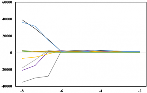
To verify the effectiveness of LASSO feature selection, our feature selection algorithm was compared with linear regression algorithm and ridge regression algorithm. Different weight coefficients were assigned to different features, such as to compare the selectivity of different algorithms. Figure 4 compares the feature coefficients selected in different cross validations.
Table 1. Segmentation results of CT image training set
|
Metric |
Method |
Mean |
Standard deviation |
|
Volume overlap error |
Reference algorithm |
5.75 |
1.52 |
|
Our algorithm |
5.69 |
1.46 |
|
|
Relative volume difference |
Reference algorithm |
1.72 |
2.31 |
|
Our algorithm |
1.35 |
0.85 |
|
|
Mean symmetric surface distance (SSD) |
Reference algorithm |
1.12 |
0.14 |
|
Our algorithm |
1.05 |
0.06 |
|
|
Root-mean-square (RMS) of SSD |
Reference algorithm |
2.14 |
0.71 |
|
Our algorithm |
1.76 |
0.55 |
|
|
Maximum SSD |
Reference algorithm |
21.46 |
5.68 |
|
Our algorithm |
18.29 |
3.48 |
|
|
Score |
Reference algorithm |
78.29 |
6.72 |
|
Our algorithm |
77.18 |
4.62 |
Table 2. Regression parameters corresponding to the selected features
|
Feature number |
1 |
2 |
3 |
4 |
5 |
6 |
7 |
|
|
|
Intercept |
β1 |
β2 |
β3 |
β4 |
β5 |
β6 |
β7 |
|
5 folds |
21.0526 |
5.3628 |
-0.8524 |
-2.2362 |
-0.1204 |
8.7129 |
-9.4152 |
0.5293 |
|
10 folds |
26.1824 |
5.2637 |
-0.8426 |
-2.4158 |
-0.0146 |
9.3685 |
-13.4852 |
0.8516 |
|
15 folds |
26.1859 |
5.1274 |
-1.1296 |
-2.1481 |
-0.7415 |
9.4851 |
-16.2937 |
1.1482 |
|
20 folds |
28.1674 |
5.1924 |
-1.3927 |
-2.1637 |
-0.0042 |
9.3562 |
-15.4297 |
1.2846 |
|
Feature number |
8 |
9 |
10 |
11 |
12 |
13 |
|
|
|
|
Intercept |
β8 |
β9 |
β10 |
β11 |
β12 |
β13 |
|
|
5 folds |
21.0526 |
-0.0421 |
-0.0326 |
4.6253 |
2 |
-16.2637 |
-0.0251 |
|
|
10 folds |
26.1824 |
-0.0748 |
-0.0126 |
4.1628 |
-1.2958 |
-14.7515 |
-0.0362 |
|
|
15 folds |
26.1859 |
-0.0182 |
-0.2618 |
4.6284 |
-2.1692 |
-16.3748 |
-0.0718 |
|
|
20 folds |
28.1674 |
-0.0418 |
-0.0812 |
4.6297 |
-2.8519 |
-1.6248 |
-0.0157 |
|
(a)
(b)
Figure 4. Feature coefficients selected in different cross validations
The restoration of the patient’s brain neural network hinges on the size change of cerebral apoplexy lesions through the rehabilitation. Therefore, this paper classifies the extracted lesion areas by size, and explores the distribution proportions of large lesion areas and small lesion areas. Figure 5 suggests that the three groups of lesion areas are roughly balanced in distribution proportion. This further demonstrates the effectiveness of our algorithm.
(a)
(b)
(c)
Figure 5. Distribution of lesions size in different classes
This paper investigates the image segmentation for review of cerebral apoplexy. Based on the correlation between image series, a segmentation method was proposed for CT images of cerebral apoplexy. The method overcomes the difficulty in segmenting the lesion areas of cerebral apoplexy and extracting the changing features of the lesion areas during the rehabilitation. Besides, a lesion area feature extraction and selection approach was developed to assist with the diagnosis of cerebral apoplexy rehabilitation, because the rehabilitation state cannot be reflected by a single feature extracted from the lesion images in the same period. Then, the segmentation results on a CT image training set were obtained, which demonstrate the high segmentation accuracy, robustness, and universality of the proposed method. In addition, the authors summarized the regression parameters corresponding to the selected features, plotted the feature coefficients selected in different cross validations, and presented the distribution of lesions size in different classes. The results show that the three groups of lesion areas are roughly balanced in distribution proportion. This further demonstrates the effectiveness of our algorithm.
[1] Lunci, Y. (2000). Fuzzy multicriteria evaluation in traditional Chinese medical diagnosis of cerebral apoplexy: An application of approximate reasoning. In PeachFuzz 2000. 19th International Conference of the North American Fuzzy Information Processing Society-NAFIPS (Cat. No. 00TH8500), Atlanta, GA, USA, pp. 211-214. https://doi.org/10.1109/NAFIPS.2000.877422
[2] Li, J., Zhao, Y., Bao, Y. (2018). Voice processing technique for patients with stroke based on chao theory and surrogate data analysis. Journal of Zhejiang University (Engineering Science), 49(1): 36-41.
[3] Kim, H., Kim, Y.L., Lee, S.M. (2015). Effects of therapeutic Tai Chi on balance, gait, and quality of life in chronic stroke patients. International Journal of Rehabilitation Research, 38(2): 156-161. https://doi.org/10.1097/MRR.0000000000000103
[4] Hoda, M., Hoda, Y., Hage, A., Alelaiwi, A., El Saddik, A. (2015). Cloud-based rehabilitation and recovery prediction system for stroke patients. Cluster Computing, 18(2): 803-815. https://doi.org/10.1007/s10586-015-0448-6
[5] Artzi, M., Aizenstein, O., Jonas-Kimchi, T., Bornstein, N., Shopin, L., Hallevi, H., Bashat, D.B., STIR and VISTA Imaging collaborators. (2014). Classification of lesion area in stroke patients during the subacute phase: A multiparametric MRI study. Magnetic Resonance in Medicine, 72(5): 1381-1388. https://doi.org/10.1002/mrm.25031
[6] van Bragt, P.J., van Ginneken, B.T., Westendorp, T., Heijenbrok-Kal, M.H., Wijffels, M.P., Ribbers, G.M. (2014). Predicting outcome in a postacute stroke rehabilitation programme. International Journal of Rehabilitation Research, 37(2): 110-117. https://doi.org/10.1097/MRR.0000000000000041
[7] Ming Lim, F., Foong, R., Yu, H. (2014). A supine gait training device for stroke rehabilitation. Journal of Medical Devices, 8(2): 020926. https://doi.org/10.1115/1.4027026
[8] Zhang, Z., Liparulo, L., Panella, M., Gu, X., Fang, Q. (2015). A fuzzy kernel motion classifier for autonomous stroke rehabilitation. IEEE Journal of Biomedical and Health Informatics, 20(3): 893-901. https://doi.org/10.1109/JBHI.2015.2430524
[9] Ostadabbas, S., Housley, S. N., Sebkhi, N., Richards, K., Wu, D., Zhang, Z., Rodriguez, M.G., Warthen, L., Yarbrough, C., Belagaje, S., Butler, A.J., Ghovanloo, M. (2016). Tongue-controlled robotic rehabilitation: A feasibility study in people with stroke. Journal of Rehabilitation Research & Development, 53(6): 98-1006. http://dx.doi.org/10.1682/JRRD.2015.06.0122
[10] Yang, K.C., Huang, C.H., Le, C.F. (2016). Applying microsoft kinect for windows to develop a Stroke Rehabilitation System. 2016 IEEE International Conference on Industrial Engineering and Engineering Management (IEEM), Bali, Indonesia, pp. 1923-1927. https://doi.org/10.1109/IEEM.2016.7798213
[11] Zondervan, D.K., Friedman, N., Chang, E., Zhao, X., Augsburger, R., Reinkensmeyer, D.J., Cramer, S.C. (2016). Home-based hand rehabilitation after chronic stroke: Randomized, controlled single-blind trial comparing the MusicGlove with a conventional exercise program. Journal of Rehabilitation Research and Development, 53(4): 457-472. https://doi.org/10.1682/jrrd.2015.04.0057
[12] Macko, R.F., Forrester, T., Francis, P., Nelson, G., Hafer-Macko, C., Roy, A. (2016). Interactive video exercise tele-rehabilitation (IVET) for stroke care in Jamaica. In 2016 IEEE Healthcare Innovation Point-Of-Care Technologies Conference (HI-POCT), Cancun, Mexico, pp. 150-153. https://doi.org/10.1109/HIC.2016.7797719
[13] Yahiaoui, A.F.Z., Bessaid, A. (2016). Segmentation of ischemic stroke area from CT brain images. In 2016 International Symposium on Signal, Image, Video and Communications (ISIVC), Tunis, Tunisia, pp. 13-17. https://doi.org/10.1109/ISIVC.2016.7893954
[14] Neethu, S., Venkataraman, D. (2015). Stroke detection in brain using CT images. Artificial Intelligence and Evolutionary Algorithms in Engineering Systems, pp. 379-386. https://doi.org/10.1007/978-81-322-2126-5_42
[15] Nurhayati, O.D., Windasari, I.P. (2015). Stroke identification system on the mobile based CT scan image. 2015 2nd International Conference on Information Technology, Computer, and Electrical Engineering (ICITACEE), Semarang, Indonesia, pp. 113-116. https://doi.org/10.1109/ICITACEE.2015.7437781
[16] Mirajkar, P.R., Bhagwat, K.A., Singh, A., Ashalatha, M.E. (2015). Acute ischemic stroke detection using wavelet based fusion of CT and MRI images. 2015 International Conference on Advances in Computing, Communications and Informatics (ICACCI), Kochi, India, pp. 1123-1130. https://doi.org/10.1109/ICACCI.2015.7275761
[17] Shieh, Y., Chang, C.H., Shieh, M., Lee, T.H., Chang, Y.J., Wong, H.F., Chin, S.C., Goodwin, S. (2014). Computer-aided diagnosis of hyperacute stroke with thrombolysis decision support using a contralateral comparative method of CT image analysis. Journal of Digital Imaging, 27(3): 392-406. https://doi.org/10.1007/s10278-013-9672-x
[18] Jeena, R.S., Kumar, S. (2013). A comparative analysis of MRI and CT brain images for stroke diagnosis. 2013 Annual International Conference on Emerging Research Areas and 2013 International Conference on Microelectronics, Communications and Renewable Energy, Kanjirapally, India, pp. 1-5. https://doi.org/10.1109/AICERA-ICMiCR.2013.6575935
[19] Ostrek, G., Przelaskowski, A. (2012). Automatic early stroke recognition algorithm in CT images. Information Technologies in Biomedicine, pp. 101-109. https://doi.org/10.1007/978-3-642-31196-3_11
[20] Tan, T.L., Sim, K.S., Chong, A.K. (2012). Contrast enhancement of CT brain images for detection of ischemic stroke. 2012 International Conference on Biomedical Engineering (ICoBE), Penang, Malaysia, pp. 385-388. https://doi.org/10.1109/ICoBE.2012.6179043
[21] Xiu, G.Y., Yuan, C.Y., Chen, X.H., Li, X.S. (2019). An innovative beam hardening correction method for computed tomography systems. Traitement du Signal, 36(6): 515-520. https://doi.org/10.18280/ts.360606
[22] Cui, H., Wang, X., Bian, Y., Song, S., Feng, D.D. (2018). Ischemic stroke clinical outcome prediction based on image signature selection from multimodality data. 2018 40th Annual International Conference of the IEEE Engineering in Medicine and Biology Society (EMBC), Honolulu, HI, USA, pp. 722-725. https://doi.org/10.1109/EMBC.2018.8512291
[23] Liu, Z., Cao, C., Ding, S., Liu, Z., Han, T., Liu, S. (2018). Towards clinical diagnosis: Automated stroke lesion segmentation on multi-spectral MR image using convolutional neural network. IEEE Access, 6: 57006-57016. https://doi.org/10.1109/ACCESS.2018.2872939
[24] Hemanth, D.J., Rajinikanth, V., Rao, V.S., Mishra, S., Hannon, N.M., Vijayarajan, R., Arunmozhi, S. (2021). Image fusion practice to improve the ischemic-stroke-lesion detection for efficient clinical decision making. Evolutionary Intelligence, 14: 1089-1099. https://doi.org/10.1007/s12065-020-00551-0
[25] Zhang, F., Zhang, C., Yang, H.M., Zhao, L. (2019). Point cloud denoising with principal component analysis and a novel bilateral filter. Traitement du Signal, 36(5): 393-398. https://doi.org/10.18280/ts.360503
[26] Kumar, A., Debnath, A., Tejaswini, T., Gupta, S., Chakraborty, B., Nandi, D. (2019). Automatic Detection of Ischemic Stroke Lesion from Multimodal MR Image. 2019 Fifth International Conference on Image Information Processing (ICIIP), Shimla, India, pp. 68-73. https://doi.org/10.1109/ICIIP47207.2019.8985923
[27] Sridharan, R., Dalca, A.V., Fitzpatrick, K.M., Cloonan, L., Kanakis, A., Wu, O., Furie, K.L., Rosand, J., Rost, N.S, Golland, P. (2013). Quantification and analysis of large multimodal clinical image studies: Application to stroke. International Workshop on Multimodal Brain Image Analysis, Nagoya, Japan, pp. 18-30. https://doi.org/10.1007/978-3-319-02126-3_3