Slow Feature Extraction Algorithm Based on Visual Selection Consistency Continuity and Its Application

In the field of image analysis and understanding, compared with fast signals, slow signals are the essential representation of invariants. They are the invariant features extracted from the high-level expression of the input high-frequency visual signals. Based on the idea of invariant learning, the slow feature analysis theory and the analysis algorithm were proposed. The algorithm is aimed to explore how to extract the slow attributes contained in high-frequency signals and the slow topology between these attributes, and has been successfully applied.

On the basis of previous studies, in 1989, Hinton [1] first proposed the basic concepts, principles and assumptions that later formed the slow feature analysis theory, and established the research foundation for slow feature analysis methods. In 2002, Wiskott and Sejnowski [2] proposed the slow feature analysis (SFA) algorithm, which conducts non-linear expansion of the feature space in an unsupervised learning manner. This algorithm effectively solved the problems of the supervised learning algorithm like insufficient sample size and constant dimensions. By this time, the theory and algorithm of slow feature analysis had been initially established, and applied research had been carried out.

In order to solve the problems in the studies on the complex cell receptive field learning models, in 2005, Berkes [3] and Wiskott applied the invariant learning results to this field and achieved great results. In 2007, Franzius et al. [4] studied the invariant relationship between hippocampal pyramidal cells and stimulation signals and revealed the stable response between the two, forming the physiological basis for the invariant learning theory.

In order to study the invariant features of the position and rotation angles of cartoon fish, in 2008, Franzius et al. [5] applied the SFA algorithm for the first time to realize invariant feature extraction and analysis, and also achieved the classification of cartoon fish based on such features. Therefore, the classification capacity of the SFA algorithm has been confirmed, laying a foundation for the theory and application of the SFA algorithm in invariant feature extraction, analysis and recognition. In order to verify the feasibility and effectiveness of the SFA algorithm in feature extraction, Kalmpfl and Maass [6] used the SFA algorithm to extract the slow features of the training data generated by the Markov chain in 2009. The test results show that: when α®o, the slow features extracted by the SFA algorithm are equivalent to those extracted by the Fisher’s Linear Discriminant FLD algorithm. In terms of feature extraction, the SFA algorithm proved to be effective and feasible, and it was also demonstrated that the training data generated by the Markov chain method have slow features.

In order to achieve the expansion of the basis function space in blind signal analysis and solve the problem of high-dimensional operation, Ma et al. [7] proposed a kernel-based slow-variation feature analysis algorithm in 2011, which achieved good performance in blind signal separation and further expanded the application field of standard SFA algorithms.

The complexity of the SFA algorithm mainly stems from the slow feature generation method, which is also a problem that scholars are generally concerned about. Inspired by the divide-and-conquer strategy, Luciw et al. [8] proposed a hierarchical slow feature analysis algorithm in 2012. The algorithm made a tradeoff between the information loss generated by the hierarchy and the complexity of the algorithm, that is, it reduced computational complexity of SFA at the cost of information loss. At the same time, the basis function family also lost its over-completeness and global features.

In order to improve the problem of information loss, Escalante-B and Wiskott [9] proposed a slow feature analysis algorithm based on graph theory (GFSA) in 2013. The research proposed the idea of using the complex structure of the training graphs to train the SFA algorithm, enabling the SFA algorithm to learn the invariance of the graph structures in the training data set and realizing the extraction of slow features and slow structures of the training set. It confirmed the dual connotations of slow features.

In 2015, Zhao et al. [10] proposed a feature extraction algorithm based on the complex visual information of natural images, which uses the custom myTICA algorithm to extract the slow features and the slow topological structures in the visual space of natural images based on visual selectivity, confirming the visual selectivity of primates determines the slow features and slow topological structures contained in natural images. In 2019, Zhao [11] bstudied an improved SFA algorithm based on visual invariance, and applied it to extract features of natural images, which achieved good results. The study confirmed the invariance of slow features and slow structures in the visual space, and the proposed algorithm proved to have good anti-noise capacity [12]. In 2020, Zhao [13] studied an improved SFA algorithm based on visual selectivity, and applied it in the feature extraction of limited defocused image sequences, which achieved good results. The study proved that in the visual space, the slow features and slow structures contained in the limited defocused image sequences are invariant, and also established an invariant feature forest.

In 2020, Zhao [14, 15] proposed an improved multi-layer LSTM algorithm based on spatial-temporal correlation, and applied it in the dynamic prediction of PM25, which achieved good results. The study proved that: in time series analysis, the improved LSTM algorithm integrating spatial features has better long-term and short-term prediction capabilities, and can realize the spatio-temporal fusion of the prediction results, which solved the problem that the traditional LSTM algorithm could not achieve the fusion of spatial features.

In recent years, the SFA algorithms have been well applied in various fields, such as human behavior recognition [16-18], blind signal analysis [7, 19], dynamic monitoring [20], 3D feature extraction [21] and multi-person path planning [22].

In summary, there has been great progress in the research on the traditional slow feature analysis (SFA) algorithm. However, it still has a number of drawbacks: 1. PCA is adopted as the feature extraction method, which ignores the visual independence between basis functions. 2. the polynomial expansion method is adopted in the expansion of basis functions, lacking the support of the computational theory of vision for primates, and making the algorithm unable to learn global features with visual selection consistency continuity, and what is more, the algorithm is highly complex. 3. The feature expression is not diversified and the slow structure of slowly-varying information is ignored.

Therefore, Slow Feature Extraction Algorithm Based on Visual selection consistency continuity and Its Application was proposed. This paper solved the drawbacks of the traditional SFA algorithm through four innovations: 1. it replaced the PCA method of the traditional SFA algorithm with the myTICA method, extracted the Gabor basis functions showing the invariance of natural images, and generated the basis function family; 2. it used the VSCC_FBEA algorithm to realize the basis function expansion of features with visual selection consistency continuity and generated an over-complete basis function family; 3. it proposed using the LOPM algorithm to optimize the over-complete basis function family, and generated the optimized over-complete basis function family; 4. It adopted the visual invariance theory -FEM to generate the set of invariable features containing the visual information of natural images and its spatial topological relations.

3.1 Analysis on the existing studies

The above sections have outlined the physiological basis for and the basic theories and implementation of the SFA algorithm, and analyzed the main reasons behind the problems of the traditional SFA algorithm. Such information is summarized in the Table 1:

Table 1. Existing research results of the SFA algorithm

The comparative study in Table 1 shows that the feature extraction method is gradually approaching the way the human brain understands the world: from PCA to MyTICA, this change achieved feature independence and the learning of spatial topological structures; the transformation in the feature expansion method, from polynomial expansion to the one based on feature probability distribution and then to the basis function expansion method based on visual invariance and visual selectivity, shows that the brain computing method has both theoretical and practical significance in the SFA basis function expansion algorithm.; and in terms of feature structure, from full features to hierarchical features and then to 3D visual information and visual spatial topological structure information, the expression of feature structure gradually approached the cognitive structure of the human brain.

Therefore, this paper made innovations in the extraction and expansion of slow feature basis functions and the generation and expression of slow spatial structures. It integrated the visual selectivity theory, the Lipschitz consistency continuity theory and the LSTM theory, proposed the LSTM algorithm based on visual selectivity as the basis function space expansion algorithm and also the LOPM algorithm to realize the effective fusion of the slow feature basis function expansion method and the visual selection consistency continuity, and predicted and extracted an over-complete basis set from natural images; and finally, it achieved the recognition of natural images. The innovations of the proposed algorithm are demonstrated in the following section one by one.

3.2 Improvements made in the proposed algorithm

Improvement 1: Receptive field model based on visual selectivity

The Gabor function can model the visual receptive field of visual cells. The four key parameters of the Gabor function realize the visual selectivity of primates’ visual cells, but with different contributions in the selective expression. In terms of contributions, the four key parameters in the descending order are frequency, orientation, phase and visual spatial position. Therefore, based on the visual selectivity theory, the Gabor model is proposed as follows:

$\left\{\begin{array}{l}\operatorname{gabor}=\operatorname{gabor}\left(\lambda_{f}, \lambda_{o}, \lambda_{p}, \lambda_{d}\right) \\ \lambda_{f}+\lambda_{o}+\lambda_{p}+\lambda_{d}=1 \\ \lambda_{f} \geq \lambda_{o} \geq \lambda_{p} \geq \lambda_{d}\end{array}\right.$    (1)

where, λ_f and λ_o respectively represent the visual spatial frequency and visual spatial orientation of the receptive field of visual cells, which play a decisive role in the visual spatial distribution process- mainly determining the type and function of the receptive field of visual cells. λ_p and λ_d respectively represent the visual space hysteresis of the visual cell receptive field and the size of the distribution area of the visual cell receptive field, which play a secondary role in the visual spatial distribution process - determining the hysteresis and positions of the intra-class visual cells.

Inspired by the theory of visual selectivity, considering the different roles (contributions) of the four parameters in the Gabor function, the normalized parametric method based on contribution is proposed as follows:

$\bar{\lambda}_{i}=\frac{\left|\lambda_{i}\right|}{\sqrt{\lambda_{f}^{2}+\lambda_{o}^{2}+\lambda_{p}^{2}+\lambda_{d}^{2}}} \quad i \in\{f, o, p, d\}$    (2)

The experimental results show that the ratio of the four parameters of the receptive field is approximately $\bar{\lambda}_{f}: \bar{\lambda}_{o}: \bar{\lambda}_{p}: \bar{\lambda}_{d}=4: 4: 1: 1$. The experimental results approximately show the contribution degrees and sizes of the four parameters.

Improvement 2: Feature extraction method based on MyTICA algorithm

The myTICA [10] method was used to replace the PCA method in the original SFA algorithm to extract the slow features of natural images, which effectively solved the problem of the original SFA algorithm that the features did not have independence and do not contain the visual spatial topological relationships. Inspired by the theory of visual selectivity, the basis functions in the family of basis functions Visual_sub_set(i) have the global and local visual selectivity obeying the rule of “similar when being close”, and form a stable spatial topological structure with close distribution. Both the slow information and the slow topology exhibit the visual selection consistency continuity. Visual_sub_set is simulated and expressed with Gabor functions as follows:

Visual_sub_set $=\left\{\right.$ Visual_sub_set $\left(p_{-}\right.$add, $\left.i\right) \mid p_{-}$add $\left.=1,2,3, \ldots, N\right\}$, $i \in\left\{\lambda_{f}, \lambda_{o}, \lambda_{p}, \lambda_{d}\right\}$    (3)

where, f represents the frequency of the receptive field, o the orientation of the receptive field, p the phase of the receptive field, d the visual spatial position of the receptive field, and N the number of elements in the basis function family.

Improvement 3: Feature basis expansion algorithm based on visual selection consistency continuity (VSCC_FBEA)

The basis space expansion of the original SFA algorithm adopted the polynomial expansion method, which has high computational complexity, lacks the support of computational theory of vision for primates, and is also unable to learn the short-term and long-term features with visual selection consistency continuity. What is more, the generated basis function space is not over-complete. Inspired by the visual selection consistency continuity calculation theory, this paper used the Gabor basis functions to model the visual receptive field. In order to obtain the long- and short-term features with visual selection consistency continuity from the frequency, orientation, phase and position of each element in the Gabor basis function family, the deep LSTM algorithm was used to replace the original polynomial expansion method, which realized the nonlinear expansion of the basis functions in the visual basis function space and their topological structure, and helped generate an over-complete basis function family and its spatial topological structure with visual selection consistency continuity.

Inspired by the theory of visual selection consistency continuity, this paper proposed the LOPM algorithm to optimize the invariant feature forest, and obtained the optimized over-complete basis function family based on visual selection consistency continuity. The detailed implementation is as follows:

Improvement 3.1 Structure of the VSCC_FBEA algorithm

Based on the above innovations, the flow chart of the feature basis expansion algorithm used in this paper is as follows Figure 1:

1.png

Figure 1. Flow chart of the VSCC_FBEA algorithm

where, the basis function space is formed by the basis functions of the natural image, which represents the visual spatial selectivity with respect to natural images, and is expressed as Visual_sub_set $=\left\{\right.$ Visual_sub_set $\left(p_{-}\right.$add,$\left.\left.i\right) \mid p_{-} a d d=1,2,3, \ldots, N\right\}, i \in\left\{\lambda_{f}, \lambda_{o}, \lambda_{p}, \lambda_{d}\right\}$; inspired by the visual selectivity rule of primates “similar when being close and different when being distant”, the basis function space is divided into basis function subspaces, expressed as Visual_sub_set $\left(p_{-} a d d\right)=\left\{\right.$ Visual_sub_set $\left.\left(p_{-} a d d, \lambda_{i}\right) \mid p_{-} a d d=1,2,3, \ldots, N ; i \in\left\{\lambda_{f}, \lambda_{o}, \lambda_{p}, \lambda_{d}\right\}\right\}$; based on the different contributions of the parameters in the basis functions, the basis function subspace Visual_sub_set(p_add) is divided into four subsets - Visual_sub_set(p_add, λ_f), Visual_sub_set(p_add, λ_o), Visual_sub_set(p_add, λ_p) and Visual_sub_set(p_add, λ_d). The counter p_add represents the dynamic curser of the basis function space, and num1 the number of elements in the basis function space. L_sample means sampling from the set Visual_sub_set(p_add, i) using the random sampling method according to the sample size L, where L is less than or equal to the number of elements in the set.

VSCC_FBEA algorithm

Improvement 3.2 Basis Fusion Algorithm (BFA algorithm)

There is a certain dependence between the four parameters of the Gabor basis function generated through prediction. Therefore, the autocorrelation and cross-correlation coefficient matrix is calculated as follows:

$\delta=\left[\begin{array}{llll}w_{f f} & w_{f o} & w_{f p} & w_{f d} \\ w_{o f} & w_{o o} & w_{o p} & w_{o d} \\ w_{p f} & w_{p o} & w_{p p} & w_{p d} \\ w_{d f} & w_{d o} & w_{d p} & w_{d d}\end{array}\right]$    (4)

This matrix describing the correlation between the four visual parameters can be used to realize the fusion of Gabor predictive parameters. The fusion algorithm (BFA algorithm) is as follows:

$\left(\bar{\lambda}_{f}, \ddot{\lambda}_{o}, \bar{\lambda}_{p}, \bar{\lambda}_{d}\right)=\left(\lambda_{f}, \lambda_{o}, \lambda_{p}, \lambda_{d}\right) \times \delta$    (5)

The four parameters $\left(\bar{\lambda}_{f}, \bar{\lambda}_{o}, \bar{\lambda}_{p}, \bar{\lambda}_{d}\right)$ generated by the BFA algorithm have learned not only the visual consistency of the basis function family, but also the correlation between the parameters. In this way, the consistency and correlation of the basis functions are integrated.

Basis Fusion Algorithm (BFA):

Improvement 3.3 Lipschitz-Orthogonal-Pruning-Method (LOPM algorithm)

Inspired by visual selectivity, among the four parameters of the Gabor function, frequency and orientation have greater contributions and play the absolute role in the Gabor function. Perform Lipschitz [25-30] conditional calculations on the frequency and orientation parameter sequences.

The frequency sequence is frequency_set $=\left\{\lambda_{f}^{1}, \lambda_{f}^{2}, \lambda_{f}^{3}, \ldots \lambda_{f}^{M}, \ldots \lambda_{f}^{N}\right\}$; and the orientation sequence is oritation_set $=\left\{\lambda_{o}^{1}, \lambda_{o}^{2}, \lambda_{o}^{3}, \ldots, \lambda_{o}^{M}, \ldots o_{o}^{N}\right\}$, where M represents the number of basis functions obtained through myICA, and from M+1 to N are the expanded basis function generated by the algorithm proposed in this paper; the parameter generated by the LSTM algorithm $\alpha=\left\{\lambda_{f}^{*}, \lambda_{o}^{*}, \lambda_{p}^{*}, \lambda_{d}^{*}\right\}$, and the calculated mean and variance (μ_f, δ_f) of the samples from frequency_set are respectively the Lipschitz coefficient L of this sequence and the constraint value of the coefficient. The calculated mean and variance (μ_o, δ_o) of the samples from Orientation_set are respectively the Lipschitz coefficient L of this sequence and the constraint value of the coefficient.

The LOPM algorithm is described as follows:

When α satisfies $\min \left(-\left(\mu_{f}-\delta_{f}\right),-\left(\mu_{o}-\delta_{o}\right)\right) \leq \lambda_{f}^{*}+\lambda_{o}^{*} \leq \min \left(\left(\mu_{f}-\delta_{f}\right),\left(\mu_{o}-\delta_{o}\right)\right)$, and $\forall \beta \in$ Gabor_set, then, if <α,β>≤ε, the vectors α and β are similar, and perform the pruning operation, and keep β. Otherwise, add α to the set Gabor_set. The pruning coefficient ε is an arbitrary small positive number that controls the complexity of pruning.

Lipschitz-Orthogonal-Pruning- Algorithm (LOPM):

Improvement 4: Feature expression method based on visual invariance theory (visual invariance theory -FEM)

The original SFA algorithm only extracts the PCA features of a natural image, which reflect the contribution of each component of the image in the whole image, but cannot show the visual consistency of the information in the visual space or the invariance of the two spatial structures of the visual information. The two spatial structures include the spatial topological invariance of each basis function family in the visual space and the topological invariance of the spatial distribution of the basis functions in the visual space.

Based on this, this paper proposed the visual invariance theory –FEM method. This is a feature expression method that can describe the visual information and the topological invariance of the information space, established based on the basis function families generated in step 1, 2, and 3 and according to the visual selection consistency continuity theory. The specific implementation process is as follows:

Basis function families with visual selection consistency continuity can be generated from each natural image - Visual_sub_set={Visual_sub_set{p_add, i}| p_add =1,2,3,…N; iÎ{λ_f, λ_o, λ_p, λ_d}}, where Visual_sub_set(p_add, i) contains N function families. According to the four parameters of visual selectivity, each function family has distinguishable visual features and visual spatial topological structures, which reflect the overall features of the global visual space; and the basis functions within each function family in the visual space also contain the visual information of the basis functions and the information of the spatial topological structure between the functions. The above-mentioned global and local visual information and the spatial topological structure information all have visual selection consistency continuity, thus forming the features with visual selection consistency continuity.

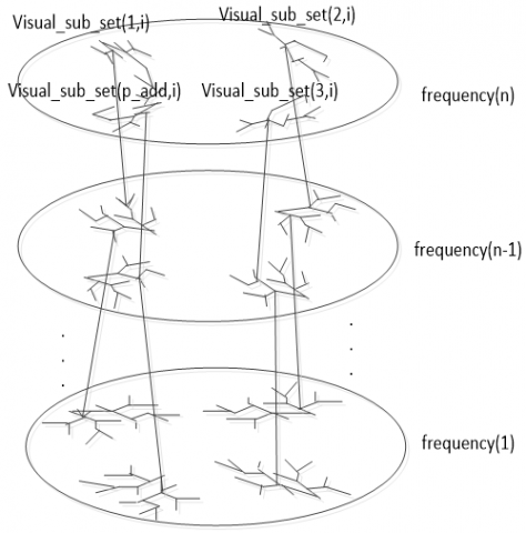
Therefore, based on the theory of visual selection consistency continuity and the theory on primates’ visual information processing – “parallel operation on the global scale and serial operation on the local scale”, a feature forest expressing the slow features and slow topologies extracted by the algorithm proposed in this paper is constructed as the following Figure 2:

2.png

Figure 2. Natural image feature forest with visual selection consistency continuity

where, Visual_sub_set(p_add, i) corresponds to the p_add-th basis function family in the visual space of the natural image, representing the local visual information of the basis function family Visual_sub_set(p_add, i). For Visual_sub_set(p_add, i), the extraction of features between basis function families is a parallel process, while the extraction of features within the same family is a serial process, which is conducive to the distributed parallel design of the algorithm. The function family Visual_sub_set expresses the global features of a natural image, including the global visual information and the global topological structure information.

In summary, the slow features of a natural image are expressed as:

$\left\{ \begin{array}{*{35}{l}}   \begin{smallmatrix}  Visual\_sub\_set\_expression=T\_encode(Visual\_sub\_set) \\  =(index(p\_add,j),gabor(p\_add,j)) \end{smallmatrix}  \\   \begin{align}  & index(p\_add,j)=T1\_encode(Visual\_sub\_set(p\_add,i,k)) \\  & gabor(p\_add,j)=T2\_encode(Visual\_sub\_set(p\_add,i,k)) \\ \end{align}  \\\end{array} \right.$    (6)

where, p_add indicates the visual space basis; j the position of the element in the visual space basis; T_encode-{T1_encode, T2_encode}; and the parameter k the basis function cursor in the basis function family. The specific coding rules are as follows:

Feature expression method based on visual invariance theory (visual invariance theory –FEM):

After the T_encode transformation, the generated matrixes Index and GM_gabor are expressed as following the Table 2:

Table 2. Feature matrix Index (with 360 features per row)

The matrix Index has frequency and orientation selectivity in the columns and rows, respectively, expressed in an ascending order, and the range of the orientation is specified as [1º, 360º]. Therefore, the features are described as the Table 3:

Table 3. Receptive field corresponding to the feature matrix (GM_gabor)

In the feature matrix Index, “1” and “0” indicate whether there is a receptive field at the location; the value “1” indicates that there is a receptive field, and there is a corresponding function Gabor(i,j) at the node of Index(i,j). These functions form the feature matrix (GM_gabor), as shown in Table 3.

5.1 Generation and display of the test gallery

According to the above theoretical analysis, the datasets for study of the parameter setting and performance of the proposed algorithm were selected from the dataset LSVRC2012. 300 classes are randomly selected from the dataset LSVRC2012, and 899 pictures were randomly selected for each class, as the training set LSVRC201_train; and the remaining 401 ones were used as the test set. Figure 4 shows some sample images selected from the gallery.

4.jpg

Figure 4. Sample pictures from the INRIA Holidays gallery for the test

5.2 Consistency of the predicted basis function

The sampling requirements are as follows: (1) the sampling size is 11´11 pixels; (2) the frequency is 2048 times; and (3) the method is random sampling. According to these requirements, a subset was selected from LSWRC201_train, which contained 899 pictures, and samples were taken from each image and formed the image set original_set. Through the execution of the algorithm [10], the visual space basis function family Visual_sub_set was generated. And through the execution of the proposed VSCC_FBEA algorithm and LOPM algorithm, the basis function family was optimized into Visual_sub_set{p_add, i}. The consistency features of the four visual selectivity parameters of the Gabor function were tested, with the results shown the Figure 5:

According to the results, the optimized basis function family Visual_sub_set{p_add, i} was generated based on the natural image set original_set by the proposed algorithm; and the consistency distribution of the four visual parameters of the basis function Gabor(f,o,p,d) with visual selectivity in the function family is shown in a) and b) of Figure 5. It can be seen that the basis function predicted and the initial basis function generated by the algorithm [10] have consistency continuity and are closely distributed in space. The basis functions in different basis function families are obviously distinguishable, with no visual selection consistency continuity. This is because, for the natural image set, the four visual parameters of the basis function Gabor (f,o,p,d) in the optimized basis function family generated by the proposed algorithm have consistency continuity, which is manifested as spatial agglomeration in the image. Therefore, the test results are consistent with the theory.

5a.png

a) Consistency distribution of frequency, orientation and position

5b.png

b) Consistency distribution of frequency, orientation and position

Figure 5. Visual consistency distribution of the predicted basis function

5.3 Effect of L in L_sampie on the prediction performance of the algorithm

In the proposed algorithm, the L_sample method consists of two parts - the value of L and the sampling method. Specifically, the value of L directly determines the number of basis functions to be sampled, and determines the nature and number of basis functions to be generated; the sampling method is related to the quality of the samples. Therefore, L_sample has significant effects on the prediction and recognition performance of the algorithm. To evaluate the prediction of the proposed algorithm with respect to the dataset LSVRC201_train, different L values were used, and the evaluation results by different methods are shown the following Table 4.

According to the test results, after the sampling method was determined, when the value of L exceeded half of the size of the basis function family Visual_sub_set{p_add, i}, that is, when L>size(Visual_sub_set{p_add, i})/2, as the value of L increased, the three evaluation indicators RMSE, MAE and MAPE decreased. The primary reason is that the increase of the L value led to an increase in the number of basis functions with visual selection consistency continuity, enhancing the learned visual selectivity features and resulting in stronger visual selection consistency continuity of the basis functions generated. In this way, the errors between basis functions decreased. Therefore, the three error-based evaluation indicators decrease with the increase of the L value.

Table 4. Relationship between the L value and the prediction performance of the algorithm

After the sampling method was determined, the change of the L value led to the change in the constraint on the generation of the basis functions, and thus the visual selection consistency continuity of the basis functions inevitably changed accordingly. When the test conditions were determined as follows:

The value range of L is [N/2,N], the step size is (NN/2)/11, and A(N)=N/2+(n-1)*(NN/2)/11; when N =2888, with the proposed algorithm executed on the dataset LSVRC201_train, the performance results of the algorithm are given as the following Figure 6 based on different L values:

6.png

Figure 6. Effect of the L value on the recognition rate of the algorithm

According to the test results, after the L-sample method was determined, with the increase of the L value, the recognition rate of the algorithm first increased and then gradually stabilized. When the L value was 2346, which means 2346 basis functions were involved in the prediction of visual selection consistency continuity (accounting for 81% of the total), the recognition performance of the algorithm approached 98.99% and tended to be stable. This indicates that, when basis functions involved in the prediction accounted for 80% or more of the elements in the basis function family, the proposed algorithm will achieve the best prediction performance. The reason is that when the proportion of basis functions exceeds 80%, the basis functions generated by the proposed algorithm through learning have very strong visual selection consistency, which increases the recognition rate of the algorithm.

In summary, when the proposed algorithm uses random sampling and the initial value of the sampling coefficient L is [0.5,1], the algorithm will have good recognition performance. In particular, when the value of L is greater than 80% of the number of elements in the basis function family, the algorithm will have a recognition rate of more than 98.99%. The above parameters can be used as the constraints for subsequent tests.

5.4 Effect of the pruning control parameter (ε) on the spatial distribution of basis functions and the recognition performance of the algorithm

The pruning control parameter ε determines whether the generated basis functions can be added to the generated basis function family, and accordingly, determines the over-completeness of the function family. Therefore, the parameter ε is essential to the prediction and recognition performance of the proposed algorithm. With different values of the parameter ε, the prediction and recognition performance of the proposed algorithm with respect to the dataset LSVRC201_train were tested, as shown the following Figure 7:

7a.png

a) Relationship between the pruning coefficient ε and the number of elements in the generated basis function family

7b.png

b) Relationship between the pruning coefficient ε and the recognition performance of the algorithm

Figure 7. Relationship between the pruning coefficient ε and the performance of the proposed algorithm

As can be seen, as the pruning control parameter ε increased, the number of elements in the generated basis function family increased, and the recognition performance of the algorithm also increased, but when ε≥0.12, the number of elements in the base function family generated by the algorithm tended to be flat, and the recognition performance of the algorithm gradually stabilized at above 97%. The primary reason is that, as the pruning control parameter ε increased, the orthogonal condition gradually relaxed, and the size of the basis function family increased accordingly. The more basis functions involved in prediction, the greater the over-completeness of Visual_sub_set{p_add, i}; and the more basis functions participating in the recognition training of the algorithm, the stronger the visual selection consistency continuity, and the better the recognition performance of the algorithm.

In summary, when ε≥0.12, the proposed algorithm can achieve the best prediction and recognition performance, with a recognition rate of 97.83%.

5.5 Feasibility evaluation of the proposed algorithm

In summary, with the respect to the training set LSVRC201_train, if the random sampling method is used, and the sampling parameter L is greater than 80% of the number of elements in the basis function family, and when the pruning control parameter ε≥0.12, the proposed algorithm can achieve the best recognition performance. The intra-class and inter-class Bhattacharyya distances are calculated, as shown in the following Figure 8.

8a.png

a) Intra-class distribution

8b.png

b) Inter-class distribution

Figure 8. Intra-class and inter-class distributed distances

According to the ROC (receiver operating characteristic) curve, when the test threshold is 8, the algorithm achieved a recognition rate of 99.66%, and both the false recognition rate and the false rejection rate are less than 0.33%. This shows that the proposed algorithm is feasible and has strong classification capacity.

5.6 Comparison of the recognition performance of different algorithms

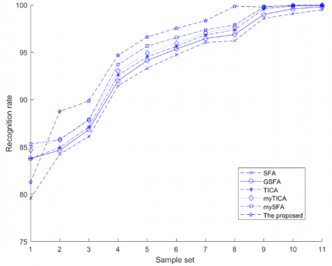
Based on the training set LSVRC201_train, by the random sampling method and with the sampling parameter L being greater than 80% of the number of elements in the basis function family and the pruning control parameter ε≥0.12, the performance of the proposed algorithm was compared with that of the other algorithms, including SFA [1], GSFA [8], TICA [9], myTICA [10] and mySFA [11]. The results are shown in Figure 9:

9.png

Figure 9. Comparison of the recognition performance of different algorithms

According to the test results, with respect to the training set LSVRC201_train, with the increase of sampling window size and sampling frequency, the size of the sample set also increased and the recognition rates of all algorithms first increased and then tended to be flat. When the sampling parameter was in the range of [7, 13], the performance of various algorithms tended to be stable, and the proposed algorithm showed a higher recognition rate than the others. The reason is that the basis functions generated by the proposed algorithm have visual selection consistency. The basis functions in the same basis function family have visual selection consistency continuity while those in different families do not, which is in line with the visual selection feature of “adjacent within one class and distant between classes”. In addition, the proposed algorithm extracts the basis functions, basis function families and their spatial topological structures in natural images, and constructs invariant information and invariant topological features in the visual space. So in essence, the above-mentioned invariant visual features are superior to those used in other algorithms. When the sampling window is too small, the visual feature information and structures presented by the basis functions extracted by the proposed algorithm will be incomplete, and thus cannot reflect the visual invariance of the basis functions; when the window is too large, the extracted area will cover multiple receptive fields, and thus the extracted basis functions will fuse the visual features of multiple receptive fields, leading to chaotic feature information of the basis functions; and when the sampling frequency is low, the visual features of natural images cannot be fully presented, and thus the information of the receptive fields is lost. All the above reasons will ultimately reduce the recognition performance of the algorithm.

In this test, the sample set was the result of optimization. The mapping relationship for the parameter is shown as the following Table 5:

Table 5. Mapping table for the sampling parameter

Table 6. Anti-noise capacity of the algorithm

5.7 Analysis on the anti-noise capacity of the algorithm (√)

The anti-noise performance is an important indicator of the robustness of an algorithm. Generally speaking, an algorithm should be able to resist different types or intensities of noise, which is also an important prerequisite for the application of the algorithm. In this paper, the type and intensity of noise have significant effects on the prediction and recognition performance of the proposed algorithm, as different noise types (Gaussian, Salt&pepper, and Speckl) and intensities have different effects on the learning of the visual selection consistency continuity of the generated basis functions. If there is too much noise, the generated basis functions will not have visual selection consistency continuity, which is not worth studying. Therefore, the noise intensity was set at [0,1,3,5,7,9,11,13,15] in the test, with % as the unit. Based on the training set LSVRC201_train, by the random sampling method and with the sampling parameter L being greater than 80% of the number of elements in the basis function family and the pruning control parameter ε≥0.12, the results of anti-noise capacity test was displayed as the Table 6.

According to the test results, when the noise intensity was in the range of [0, 15%], the recognition rate of the algorithm decreased as the noise intensity increased. When the noise intensity was between [0, 5%], the recognition rate of the algorithm decreased slowly as the noise intensity increased; and when it exceeded this range, the recognition rate decreased rapidly as the noise intensity increased. In terms of noise types, the functional expression of Gaussian noise is a subset of the Gabor function, which has obvious visual “ON-OFF” selectivity. Therefore, the increase of Gaussian noise will have two effects: (1) increasing the basis functions; (2) changing the features of the basis functions. It will directly result in the inability of the extracted basis functions to reflect the essential features of natural images. However, the visual selection consistency pruning technology of the proposed algorithm is able to eliminate these basis functions, so the increase of this type of noise has little effect on the overall performance of the algorithm. Salt & pepper noise, featured by black and white dots, has minor visual “ON-OFF” selectivity. This type of noise can change the visual features of a natural image within a region, thereby affecting the regional learning ability of the Gabor basis function. With the increase of the sampling window size, the impact will gradually become smaller, but the pruning technology used in the proposed algorithm has no obvious mitigating effect on this type of noise. Unlike the previous two types of noise, Speckl noise has larger monomer structures and can independently form Gabor basis functions with visual selectivity, so it can change the visual features and visual spatial topological structures of a natural image within a region in a fused manner. The visual features extracted by the proposed algorithm are fused features instead of the visual features of natural images. Therefore, this type of noise has great impact on the recognition rate of the proposed algorithm. In summary, under the same noise intensity, the sequence of the noise types is Speckl, Salt&pepper and Gaussian noise in terms of their impacts on the recognition rate of the proposed algorithm from high to low.