Dan Chen* | Jiali Tang | Haixu Xi | Xiaorong Zhao
© 2021 IIETA. This article is published by IIETA and is licensed under the CC BY 4.0 license (http://creativecommons.org/licenses/by/4.0/).
OPEN ACCESS
The accurate judgement of fruit maturity is significant for modern agriculture. At present, few scholars have monitored and recognized fruit maturity based on the Internet of things (IoT) and image recognition technology. Therefore, this paper explores the image recognition of fruit maturity in the context of agricultural Internet of things (IoT). Firstly, the single shot multi-box detection (SSD) algorithm was improved for fruit recognition and positioning, and used to determine the size and position the fruits to be recognized. Next, an image fusion algorithm was designed based on improved Laplacian pyramid, which effectively compresses the large fruit monitoring images shot in the same scene. The proposed algorithm was proved feasible and effective through experiments.
internet of things (IoT), image processing, modern agriculture, fruit maturity
The fruit picking time mainly depends on the maturity of the fruit [1-3]. Fruits of different usages should be picked at different stages of maturity. The picking time needs to be properly advanced or delayed, according to the specific usage [4-7]. Due to the limitations of warehousing and logistics, fruits should not be picked when they are too mature or raw. The accurate judgement of fruit maturity is significant for modern agriculture [8, 9]. The Internet of things (IoT) helps to acquire information from fruit detection terminals in orchards, and evaluate the fruit maturity. Meanwhile, image recognition can determine the size and position fruits [10-14]. The advancement of the two techniques makes the monitoring of fruit growth and insect attack more intelligent and automatic in modern agriculture.
Manual measurement/grading often fails on oil palm fruits. Syaifuddin et al. [15] collected palm fruit colors based on gray-level co-occurrence matrices (GLCMs), extracted the color features of palm fruits through regression, and thus detected the maturity of these fruits. Zheng et al. [16] adopted artificial neural network (ANN) to recognize the maturity of citrus fruits in Xinhui, China, and experimentally verified that the proposed algorithm is a non-contact, low-cost, easy-to-achieve, and high-performance method for remote monitoring. The algorithm facilitates the record of citrus growth and forecast of market sales, contributing greatly to agricultural production.
Tomato maturity is closely related to its surface color. Dimatira et al. [17] treated color, size, and shape as the metrics of tomato maturity, evaluated the maturity level of tomatoes by machine vision, and divided the colors of the fruits into six phases: green phase, crushing phase, transition phase, pink phase, and light red phase. To realize real-time accurate recognition of the maturity of fruits and vegetables, Fadhel and Al-Shamma [18] proposed a field programmable gate array (FPGA) as the parallel hardware structure, aiming to reduce the high time cost of color thresholding and k-means clustering (KMC). Xiao et al. [19] predicted the maturation stage of tomato fruits according to surface color, and managed to forecast the surface color variation based on temperature conditions. Cai and Zhao [20] developed a mature fruit recognition technique in natural scenes, which compares the color models of hue-saturation-intensity (HSI) system. The technique can fuse tone and saturation data into a fused image, in order to eliminate the effects of soil and sky backgrounds on recognition.
Overall, the fruit maturity recognition techniques at home and abroad are mostly theoretical. Few of them have been applied in practice. Not many scholars have combined the IoT with image recognition for fruit maturing monitoring and recognition in complex orchid environments. To solve the problem, this paper explores the image recognition of fruit maturity in the context of agricultural IoT. Section 2 improves the single shot multi-box detection (SSD) algorithm for fruit recognition and positioning, and completes the determination of the size and position the fruits to be recognized. Section 3 designs an image fusion algorithm based on improved Laplacian pyramid, which effectively compresses the large fruit monitoring images shot in the same scene. The proposed algorithm was proved feasible and effective through experiments.
2.1 SSD model construction
The extensive research and application of machine vision and IoT effectively improve the efficiency of various tasks on modern agricultural product picking lines, including fruit type recognition, maturity identification, fast picking, rapid sorting, fast packing, etc. In the automatic picking scenes of agricultural products, there are a huge number of various fruits, and the picking environment is extremely complex. These pose an immense challenge to the size and maturity detection of fruits.
The automation of agricultural picking is premised on the effective recognition of fruits and their maturity in complex background. This paper chooses to construct an SSD target detection model, in order to determine the size and position of the fruits to be recognized. The SSD model, which is based on feature pyramid network (FPN), is an end-to-end target detection framework, capable of detecting fruits of various sizes. The model regards feature map cells of different resolutions as priori boxes with different sizes and aspect ratios, and predicts the targets’ bounding boxes based on the priori boxes.
The SSD model consists of a feature layer CL4-3 and a series of additional convolutional layers. The feature layer is obtained through feature extraction of VGG16. The convolutional layers cover feature layers CL7, CL8-2, CL9-2, CL10-2, CL11-2.
The SSD model can calculate the confidence for the position of the detection frame and the class of fruit size corresponding to each prior box. Let p=(pda, pdb, pq, pg) be the position of a prior box; r=(rda, rdb, rq, rg) be a bounding box. Then, the relationship of the predicted bounding box k=(kda, kdb, kq, kg) for the target fruit with r and p can be expressed as:
${{k}^{da}}=\left( {{r}^{da}}-{{p}^{da}} \right)/{{p}^{q}}$ (1)
${{k}^{db}}=\left( {{r}^{db}}-{{p}^{db}} \right)/{{p}^{g}}$ (2)
${{x}_{1,2}}\,=\,\frac{-b\pm \sqrt{{{b}^{2}}-4ac}}{2a}$ (3)
${{k}^{g}}=log\left( {{r}^{g}}/{{p}^{g}} \right)$ (4)
To predict the bounding box of a fruit, the above encoding process needs to be reversed, that is, the bounding box needs to be decoded.
Let d be the number of predicted classes for the target fruit; N×M be the size of the feature map; NM be the number of cells in the feature map; l be the number of prior boxes corresponding to each cell. Then, each unit will output (d+4)l predicted bounding boxes, and the feature map will output a total of (d+4)lNM predicted bounding boxes.
In this paper, the feature map for prediction has N feature layers of different sizes. Let Emin and Emax be the minimum and maximum dimension scales of the feature layers, respectively. The feature layers of different sizes generate prior boxes with different aspect ratios. The ratio of each prior box to the original image can be calculated by:
${{E}_{l}}={{E}_{min}}+\frac{{{E}_{max}}-{{E}_{min}}}{N-1}\left( l-1 \right)l\in \left[ 1,N \right]$ (5)
Let qβl and gβl be the width and height of the prior box, respectively; βs be the default aspect ratio of the box. Then, the width of the prior box can be calculated by:
$q_{l}^{\beta }={{E}_{l}}\sqrt{{{\beta }_{s}}}$ (6)
The height of the prior box can be calculated by:
$g_{l}^{\beta }={{E}_{l}}/\sqrt{{{\beta }_{s}}}$ (7)
Let m be the number of positive samples for the matching between the target box and predicted box; $a \in\{1,0\}$ be the binary function reflecting whether the two boxes match each other (if yes, a=1; otherwise, a=0); h be the position of actual target box; ζ be the weight coefficient about the proportional relationship of position loss and confidence loss. In this paper, the sum of the position error KL and the class confidence error KC of the detection frame is defined as the loss function of SSD model:Let m be the number of positive samples for the matching
$Loss\left( a,d,k,h \right)=\frac{1}{m}\left( {{K}_{C}}\left( a,d \right)+\zeta {{K}_{L}}\left( a,k,h \right) \right)$ (8)
Because the model adopts the cross-entropy loss function, the output probabilities of different fruit classes need to be calculated through softmax regression of class confidence. Let aijo be the indicator of whether the i-th prior box matches the j-th actual box in class O; dio be the confidence of the i-th prior box belonging to class O; ḋio and ḋi0 be the confidence of softmax regression and background of the i-th prior box, respectively; ZS and FS be the set of positive samples, and the set of negative samples, respectively. Then, the class confidence error KC can be calculated by:
${{K}_{C}}\left( a,d \right)=-\sum\limits_{i\in ZS}^{m}{a_{ij}^{o}log\left( \dot{d}_{i}^{o} \right)}-\sum\limits_{i\in FS}{log\left( \dot{d}_{i}^{0} \right)}$ (9)
ḋio can be calculated by:
$\dot{d}_{i}^{o}=\frac{exp\left( \dot{d}_{i}^{o} \right)}{\sum\nolimits_{o}{exp\left( \dot{d}_{i}^{o} \right)}}$ (10)
The position error of the detection frame can be characterized by Smooth-L1 loss function:
${{K}_{smooth-{{L}_{1}}}}\left( a \right)=\left\{ \begin{align} & 0.5{{a}^{2}}\text{ }\left| a \right|<1 \\ & \left| a \right|-0.5\text{ } otherwise \\ \end{align} \right.$ (11)
Let pdai, pdbi, pqj, and pgi be the central coordinates, width, and height of the i-th prior box, respectively; ḣdaj, ḣdbj, ḣqj, and ḣgi be the central coordinates, width, and height of the actual box of the target fruit, respectively. The deviations of the actual box from the prior box can be calculated by:
$\dot{h}_{j}^{da}=\left( h_{j}^{da}-p_{i}^{da} \right)/p_{i}^{q}$ (12)
$\dot{h}_{j}^{db}=\left( h_{j}^{db}-p_{i}^{db} \right)/p_{i}^{g}$ (13)
$\dot{h}_{j}^{q}=log\left( h_{j}^{q}/p_{i}^{q} \right)$ (14)
$\dot{h}_{j}^{g}=log\left( h_{j}^{g}/p_{i}^{g} \right)$ (15)
The deviations obtained by formulas (12)-(15) can be transformed to derive the position of the prior box.
2.2 SSD model construction based on residual network
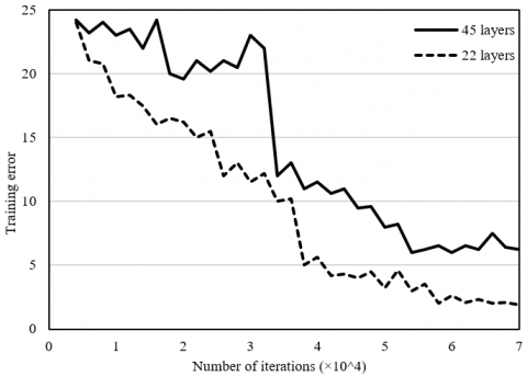
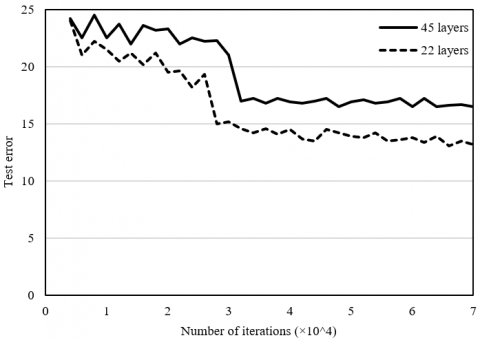
Before introducing the residual network, SSD target detection model could contain 22 layers at the most. The network depth needs to be properly increased for better recognition and positioning effects. Figure 1 shows the relationship between training error, test error, and number of network layers. It can be seen that the training error and test error increase with the growing number of layers. In a network with more layers, the training and test errors of fruit recognition descend faster. Therefore, over-fitting will not cause the two errors to rise. In theory, it is not wise to build a deep network simply by stacking several nonlinear layers. A better strategy is to add an identity mapping layer to the constructed network, or fit the ideal identity mapping based on a series of nonlinear networks. Figure 2 shows the structure of the residual learning unit that helps the neural network fit identity mapping.
(a) Relationship between training error and number of network layers
(b) Relationship between test error and number of network layers
Figure 1. Relationship between training error, test error, and number of network layers
Figure 2. Structure of residual learning unit
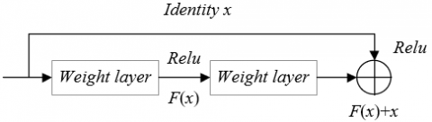
Figure 3 shows the structure of SSD target detection model based on residual network. In the model, the area in the input image corresponding to a point on a feature map changes with the sizes of the feature map. To select the default box parameters for the target fruit, the size and position of different fruits should correspond to the default box at different positions. Based on formula (5), Emin was set to 0.2, Emax to 0.95, and default aspect ratio to βs={1, 2, 3, 0.5, 0.33}. Let sl be the size of the l-th feature map. Then, the central coordinates of the default box can be configured as:
$\left( \frac{i+0.5}{{{s}_{l}}},\frac{j+0.5}{{{s}_{l}}} \right)$ (16)
Figure 3. Structure of SSD target detection model based on residual network
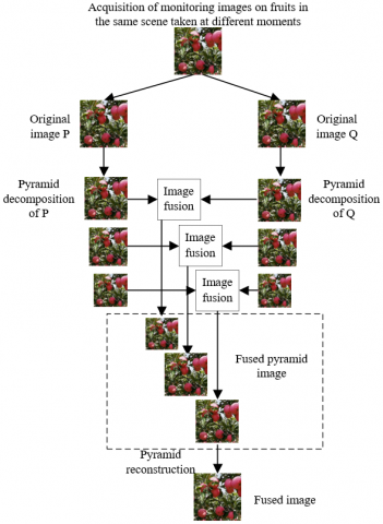
With the progress of science and technology, the integration between the IoT and image recognition open new directions to maturity monitoring of agricultural fruits. For example, wireless sensor network (WSN) can detect maturity information like fruit size and color via multimedia visual nodes, and transmit the data on fruit maturity to the data processing center through wireless communication, realizing the full detection of fruit maturity across the orchard. Fruit growth is a long process. During the growth period, the monitoring system shots a huge number of images on the same scene, calling for effective compression. This paper introduces image fusion to synthetize the multiple images taken by the monitoring system on the same scene into a new higher quality image, which demonstrates the fruit maturity in an all-round way. The synthesis effectively enhances the image usability.
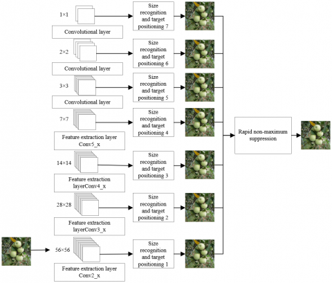
The traditional image fusion approaches are based on blocks or pixels. Despite enhancing the direct correlations between adjacent pixels, the traditional methods affect the finer visual effects, such as the size changes of the targets. This paper proposes an image fusion algorithm based on improved Laplacian pyramid. The algorithm can fuse images on different feature layers decomposed from the original image, offering a better alternative for analyzing image details. Figure 4 shows the flow of image fusion algorithm based on pyramid decomposition.
Figure 4. Flow of fruit image fusion algorithm for agricultural IoT
Let H0 be an original monitoring image of fruits; N be the number of feature layers in each original image. Then, the process of Gaussian pyramid decomposition is detailed first:
Firstly, a low-pass window function WF(x, y) is convoluted with the k-1-th feature layer Hk-1 of the original image. Then, down-sampling is performed on the convolution result every other row and every other column:
${{H}_{k}}=\sum\limits_{x=-2}^{2}{\sum\limits_{y=-2}^{2}{WF\left( x,y \right){{H}_{k-1}}\left( 2i+x,2j+y \right)}}$ (17)
where, WF(x, y) is a 5×5 low-pass filter. Let DSk and HSk be the number of columns and rows in the sub-image on the k-th layer of Gaussian pyramid. Then, k, i and j satisfy 0<k≤N, 0≤i<DSk, and 0≤j<HSk, respectively.
WF(x, y) meets four constraints at the same time: separability, normalizability, symmetry, and equal contribution between odd and even terms. Let g be the Gaussian density distribution function. The separability constraint can be expressed as:
$WF(x, y)=g(x)*g(y)$ (18)
The normalizability constraint can be expressed as:
$\sum\limits_{N=-2}^{2}{g(x)}=1$ (19)
The symmetry constraint can be expressed as:
$ g\left( i \right)=g\left( -i \right)$ (20)
The constraint of equal contribution between odd and even terms can be expressed as:
$g\left( 0 \right)+g\left( -2 \right)+g\left( +2 \right)=g\left( -1 \right)+g\left( +1 \right)$ (21)
Under the above four constraints, we have:
$\left\{ \begin{matrix} g\left( 0 \right)=0.375 \\ g\left( -1 \right)=g\left( +1 \right)=0.25 \\ g\left( -2 \right)=g\left( +2 \right)=0.0625 \\ \end{matrix} \right.$ (22)
Under the separability constraint (18), the window function WF(x, y) can be calculated by:
$WF=\left[ \begin{matrix} \frac{1}{256} & \frac{1}{64} & \frac{1}{42} & \frac{1}{64} & \frac{1}{256} \\ \frac{1}{64} & \frac{1}{16} & \frac{1}{11} & \frac{1}{16} & \frac{1}{64} \\ \frac{1}{42} & \frac{1}{11} & \frac{1}{7} & \frac{1}{11} & \frac{1}{42} \\ \frac{1}{64} & \frac{1}{16} & \frac{1}{11} & \frac{1}{16} & \frac{1}{64} \\ \frac{1}{256} & \frac{1}{64} & \frac{1}{42} & \frac{1}{64} & \frac{1}{256} \\ \end{matrix} \right]$ (23)
The Gaussian pyramid image sequence can be described as H0, H1, …, HN. Starting with each original image, the image Hk of the previous feature layer is processed through low-pass filtering and down-sampling to obtain the feature map Hk-1 of the current layer. The final Gaussian pyramid image is composed of the feature maps in ascending order. The top and bottom layers are HN and H0, respectively. The total number of layers is N+1.
After obtaining the Gaussian image pyramid, interpolation is adopted to expand the image Hk on the k-th feature layer, while ensuring that the expanded image H'k is of the same size as the feature image Hk-1 on layer l-1:
${{{H}'}_{k}}=EX\left( {{H}_{k}} \right)$ (24)
The expansion operator EX can be defined as:
${{{H}'}_{k}}\left( i,j \right)=4\sum\limits_{x=-2}^{2}{\sum\limits_{y=-2}^{2}{WF\left( x,y \right)H_{k}^{*}\left[ \frac{x+i}{2},\frac{y+j}{2} \right]}}$ (25)
where,
$H_{k}^{*}\left(\frac{x+i}{2}, \frac{y+j}{2}\right)$
$=\left\{\begin{array}{l}H_{k}\left(\frac{x+i}{2}, \frac{y+j}{2}\right), \text { if } \frac{x+i}{2} \text { and } \frac{y+j}{2} \text { are integers } \\ 0, \text { otherwise }\end{array}\right.$ (26)
The image IMk on the k-th feature layer in the Laplacian pyramid, which is generated from Gaussian pyramid, can be given by:
$I{{M}_{k}}={{H}_{k}}-{{{H}'}_{k}}$ (27)
$I{{M}_{N}}={{H}_{N}}$ (28)
The complete Laplacian pyramid is composed of the image sequence IM0, IM1, …IMm, which can be reconstructed by:
${{H}_{k}}=I{{M}_{k}}+{{{H}'}_{k}}$ (29)
From the top of the Laplacian pyramid, each layer is deduced by formula (29) until k=0. In this way, the original image on the target fruit can be reconstructed. To a certain extent, the image reconstructed through traditional Laplacian transform is influenced by the coefficient noise of the transform domain. Therefore, the reconstructed image is not necessarily the optimal image.
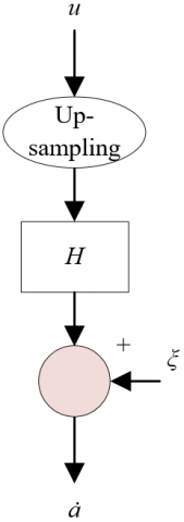
The traditional Laplacian reconstruction algorithm can be expressed as:
${{\dot{a}}_{T}}=H\cdot u+\xi $ (30)
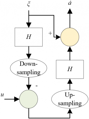
This paper improves the Laplacian pyramid algorithm for image reconstruction:
${{\dot{a}}_{2}}=H\cdot u+\left( 1-HP \right)\xi $ (31)
Figure 5 compares the reconstruction processes of the original and improved algorithms. The two algorithms process the difference signal ξ differently. The original algorithm directly superposes ξ values, while the improved algorithm superposes the projections of ξ. The improved algorithm outperforms the original algorithm, because it can effectively eliminate the influence of some errors, when the transform domain coefficients are noisy.
|
(a) Original reconstruction algorithm |
(b) Improved reconstruction algorithm |
Figure 5. Reconstruction processes of the original and improved algorithms
After Laplacian pyramid transform, each original image is decomposed into different spatial frequency bands. Then, the detailed features are extracted from each layer of the decomposed image, using different fusion operators based on regional features.
For original images P and Q, the images on the k-th layer decomposed by Laplacian pyramid are denoted as IPk and IQk, respectively; the fused image is denoted as ISk(0≤k≤N). For an image, the greater the mean gradient, the more obvious the changes to the edges of the target, and the easier it is to extract target size. Therefore, this paper fuses the top-level images through local mean gradient method. Suppose x and y are two odd numbers no smaller than 3. Then, the mean gradient is calculated for the x×y area centering on each pixel of the image. Let ΔJa and ΔJb be the first-order differences of pixel PI(a, b) in directions a and b, respectively. Then, we have:
$AG=\frac{1}{\left( x-1 \right)\left( y-1 \right)}\sum\limits_{i=1}^{x-1}{\sum\limits_{j=i}^{y-1}{\sqrt{\left( \Delta J_{a}^{2}+\Delta J_{b}^{2} \right)/2}}}$ (32)
ΔJa and ΔJb can be respectively defined as:
$\Delta {{J}_{a}}=PI\left( a,b \right)-PI\left( a-1,b \right)$ (33)
$\Delta {{J}_{b}}=PI\left( a,b \right)-PI\left( a,b-1 \right)$ (34)
The fused image can be expressed as:
$I{{S}_{k}}\left( i,j \right)=\left\{ \begin{align} & I{{P}_{k}}\left( i,j \right)\text{ }HP\left( i,j \right)\ge HQ\left( i,j \right) \\ & I{{Q}_{k}}\left( i,j \right)\text{ }HW\left( i,j \right)\le HQ\left( i,j \right) \\ \end{align} \right.$ (35)
This paper fuses the non-top-layer decomposed images with 0≤k≤N with area energy method. Firstly, the area size is set to 3×3, and weighting coefficient to ω(γ, θ). Then, the energy of the local area LAEk (i, j) centering at (i, j) on the k-th layer of Laplacian pyramid can be calculated by:
$LA{{E}_{k}}\left( i,j \right)=\sum\limits_{\gamma =-1}^{1}{\sum\limits_{\theta =-1}^{1}{\omega \left( \gamma ,\theta \right){{\left[ {{\psi }_{i}}\left( i+\gamma ,j+\theta \right) \right]}^{2}}}}$ (36)
The matching degree of the local area LAMk (i, j) can be expressed as:
$\begin{align} & LA{{M}_{k}}\left( i,j \right) \\ & =\frac{\sum\limits_{\gamma =-1}^{1}{\sum\limits_{\theta =-1}^{1}{\omega \left( \gamma ,\theta \right){{\psi }_{i,P}}\left( i+\gamma ,j+\theta \right){{\psi }_{i,Q}}\left( i+\gamma ,j+\theta \right)}}}{LA{{E}_{k,P}}\left( i,j \right)+LA{{E}_{k,Q}}\left( i,j \right)} \\ \end{align}$ (37)
Next is to define the matching threshold φ for images. In an area, if the matching degree between two images is smaller than φ, then the two images have great differences. In this case, the central pixel in an area with large local area energy can be selected as the central pixel of the image fused from the two images. If the matching degree between two images is greater than φ, then the two images have little differences. In this case, the gray value of the area in the fused image can be determined by weighted fusion algorithm. If LAMk (i, j)<φ, then:
$\left\{ \begin{align} & {{\psi }_{k,S}}\left( i,j \right)={{\psi }_{k,P}}\left( i,j \right),LA{{M}_{k,P}}\left( i,j \right)\ge LA{{M}_{k,Q}}\left( i,j \right) \\ & {{\psi }_{k,S}}\left( i,j \right)={{\psi }_{k,Q}}\left( i,j \right),LA{{M}_{k,P}}\left( i,j \right)<LA{{M}_{k,Q}}\left( i,j \right) \\ \end{align} \right.$ (38)
When LAMk (i, j)≥φ, if LAEk,P (i, j)>LAEk,Q(i, j), we have:
$\begin{align} & {{\psi }_{k,S}}\left( i,j \right)={{\mu }_{k,max}}\left( i,j \right){{\psi }_{k,P}}\left( i,j \right) \\ & +{{\mu }_{k,min}}\left( i,j \right){{\psi }_{k,Q}}\left( i,j \right) \\ \end{align}$ (39)
If LAEk,P (i, j)<LAEk,Q(i, j), we have:
$\begin{align} & {{\psi }_{k,S}}\left( i,j \right)={{\mu }_{k,min}}\left( i,j \right){{\psi }_{k,P}}\left( i,j \right) \\ & +{{\mu }_{k,max}}\left( i,j \right){{\psi }_{k,Q}}\left( i,j \right) \\ \end{align}$ (40)
where, μk,min (i, j) and μk,max (i, j) are weighted fusion operators:
$\left\{ \begin{matrix} {{\mu }_{k,min}}\left( i,j \right)=\frac{1}{2}-\frac{1}{2}\left( \frac{1-LA{{M}_{k}}\left( i,j \right)}{1-o} \right) \\ {{\mu }_{k,max}}=1-{{\mu }_{k,min}}\left( i,j \right) \\ \end{matrix} \right.$ (41)
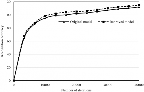
Figure 6. Recognition accuracy curves
To test the convergence and fruit recognition accuracy of the improved SSD target detection model, this paper designs a comparative experiment between the original SSD and the improved SSD on a dataset of fruit maturity monitoring samples in the context of agricultural IoT. Figures 6 and 7 show the recognition accuracy curves and the relationship between the number of fruits and recognition accuracy, respectively.
As shown in Figure 6, within 4,000 iterations, the original and improved SSD models differed slightly in the recognition rate curve of the fruits in the dataset. After 10,000 iterations, the improved SSD model achieved a slightly higher recognition rate than the original model. As shown in Figure 7, the recognition accuracy is negatively correlated with the number of fruits in each monitoring image. Therefore, a small number of fruits per image benefits the fruit recognition accuracy. The improved SSD model greatly enhances the accuracy of fruit recognition. When the number of fruits was greater than 2, the improved SSD achieved a much higher recognition rate than the original model. When the number increased to 7, the recognition rate of the improved SSD was still greater than 90%.
The accuracy and recall of positive samples (Figure 8) show that our agricultural IoT-driven fruit recognition method clearly outshined the traditional SSD and R-CNN, a CNN-based regional method, in the accuracy and recall of positive samples. Our method had no significant error, although it was not as good as the traditional SSD in the extraction of the maturity features of a few fruits. The improved SSD optimizes the feature extraction from fruits with size and shape changes.
Figure 7. Relationship between the number of fruits and recognition accuracy
(a) Accuracy
(b) Recall
Figure 8. Accuracy and recall of positive samples
Note: R-CNN is short for region-based convolutional neural network.
Next, the above three models were compared against several metrics of size estimation and positioning effect (Table 1). On positive samples, the proposed improved SSD model achieved an accuracy of 93.74%, a recall of 92.65%, an F1-score of 93.56%, a Cohen’s kappa coefficient of 93.89%, and a mean accuracy (MA) of 93.15%. The MA of our model was 3.33% and 1.26% higher than the original SSD and R-CNN, respectively. Overall, our SSD model slightly outperforms the other two models.
Next, the authors further examined how the number of layers decomposed by Laplacian pyramid in the agricultural IoT-driven fruit image fusion algorithm influences the fusion quality. Our method was applied to fuse the monitoring images on fruit maturity. Table 2 presents the fused image quality at different number of layers. The relationship between the number of layers and four objective metrics of image fusion effect can be observed from the table, including MSE, mutual information, cross entropy, and peak S/N. The four metrics gradually improved with the increasing number of layers. Considering the effect of computing load, this paper sets the number of layers decomposed by Laplacian pyramid to five.
Table 1. Performance metrics of three models
|
Metric |
Traditional SSD |
R-CNN |
Our model |
|
Accuracy |
90.72 |
92.57 |
93.74 |
|
Recall |
91.75 |
91.35 |
92.65 |
|
F1-score |
91.46 |
91.46 |
93.56 |
|
Cohen’s kappa coefficient |
91.34 |
91.52 |
93.89 |
|
MA |
91.26 |
92.63 |
93.15 |
Table 2. Fused image quality at different number of layers
|
Number of layers |
MSE |
Mutual information |
Cross entropy |
Peak S/N |
|
2 |
5.3246 |
5.0721 |
0.0600 |
33.6759 |
|
3 |
2.7984 |
5.3256 |
0.0185 |
39.5031 |
|
4 |
1.8823 |
5.2470 |
0.0075 |
42.8254 |
|
5 |
1.8675 |
5.2768 |
0.0068 |
42.1762 |
Note: MSE is short for mean squared error; S/N is short for signal-to-noise ratio.
After that, a contrastive experiment was carried out on two clear images taken with an interval of 1 week in the dataset of fruit maturity monitoring images. The fusion results of five fusion algorithms were compared, including traditional Laplacian transform, wavelet transform, multiscale transform, Ridgelet transform, and our algorithm. The performance of these algorithms is compared in Table 3, using metrics like mean gradient, information entropy, and peak S/N.
Table 3. Image fusion performance of five different algorithms
|
Name of algorithm |
Mean gradient |
Information entropy |
Peak S/N |
|
Traditional Laplacian transform |
2.4356 |
6.8572 |
30.1578 |
|
Wavelet transform |
2.7523 |
6.7534 |
33.6842 |
|
Multiscale transform |
2.6862 |
7.0239 |
33.7595 |
|
Ridgelet transform |
2.6714 |
7.0458 |
33.8267 |
|
Our algorithm |
2.7527 |
7.1275 |
35.7653 |
As shown in Table 3, the fused images obtained through traditional Laplacian transform and traditional wavelet transform had problems like dimness, unclarity, ghosting, and noises, i.e., the two algorithms achieved poor fusion effects. Multiscale transform realized better fusion effect than the two algorithms, but did not output sufficient clarity. The images fused by Ridgelet transform had fuzzy edges. Compared with the other methods, our algorithm can fully preserve the details of the original images, and improve the subjective visual effects of fruit edges.
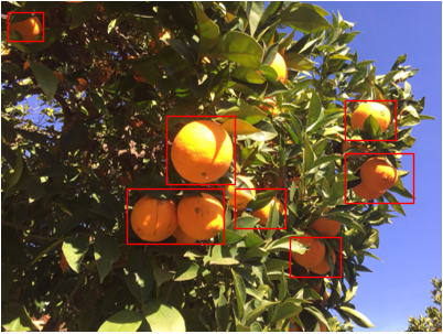
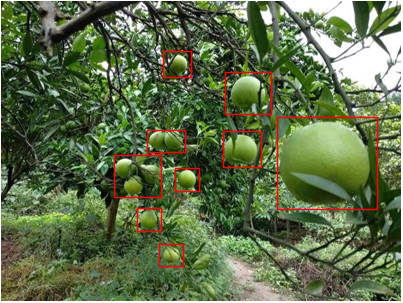
A total of 250 fruit images taken in six months were fused by our model to verify its performance of maturity recognition. Our model spent 213.10s recognizing all images, that is, 0.852s on each image. Figure 9 visualizes some of the detection results. The recognition rates in the red boxes are the final recognition results on orange maturity.
|
(a) |
(b) |
Figure 9. Recognition effects of fruit maturity
This paper probes into the image recognition of fruit maturity in the context of agricultural IoT. The SSD was improved to accurately recognize the size and position of each target fruit. Next, the improved Laplacian pyramid was adopted to design an image fusion algorithm, which effectively compresses the large fruit monitoring images shot in the same scene. After that, the authors experimentally obtained the recognition accuracy curves, and further explored the relationship between the number of fruits and recognition accuracy. Furthermore, the accuracy and recall on positive samples, and recognition performance of multiple models were compared. The comparison shows that our model outperformed the other models in positive sample accuracy, recall, F1-score, Cohen’s kappa coefficient, and MA. Finally, the performance of different image fusion algorithms was contrasted, revealing that our algorithm can fully preserve the details of the original images, and improve the subjective visual effects of fruit edges.
This work is funded by the National Social Science Fund of China (Project Title: Construction and Application of Mobile Library Service Model Based on Context-aware, Grant No.: 19BTQ045).
[1] Hu, B., Sun, D.W., Pu, H., Wei, Q. (2019). Recent advances in detecting and regulating ethylene concentrations for shelf-life extension and maturity control of fruit: A review. Trends in Food Science & Technology, 91: 66-82. https://doi.org/10.1016/j.tifs.2019.06.010
[2] Chandra, T.G., Erwandha, K.G., Aditya, Y., Priyantari, B.A., Fitriani, D., Hakim, M.H., Hidayat, A.S., Hatta, A.M., Irawati, N. (2019). Tomatoes selection system based on fruit maturity level using digital color analysis method. In Third International Seminar on Photonics, Optics, and Its Applications (ISPhOA 2018), Surabaya, Indonesia. https://doi.org/10.1117/12.2504987
[3] Sukrisno, E. (2019). Identification using the K-Means clustering and gray level co-occurance matrix (GLCM) at maturity fruit oil head. 2019 Fourth International Conference on Informatics and Computing (ICIC), Semarang, Indonesia. https://doi.org/10.1109/ICIC47613.2019.8985681
[4] Takahashi, M., Hirose, N., Ohno, S., Arakaki, M., Wada, K. (2018). Flavor characteristics and antioxidant capacities of hihatsumodoki (Piper retrofractum Vahl) fresh fruit at three edible maturity stages. Journal of Food Science and Technology, 55(4): 1295-1305. https://doi.org/10.1007/s13197-018-3040-2
[5] Tolesa, G.N., Workneh, T.S., Melesse, S.F. (2018). Modelling effects of pre-storage treatments, maturity stage, low-cost storage technology environment and storage period on the quality of tomato fruit. CyTA-Journal of Food, 16(1): 271-280. https://doi.org/10.1080/19476337.2017.1392616
[6] VanderWeide, J., Medina-Meza, I.G., Frioni, T., Sivilotti, P., Falchi, R., Sabbatini, P. (2018). Enhancement of fruit technological maturity and alteration of the flavonoid metabolomic profile in Merlot (Vitis vinifera L.) by early mechanical leaf removal. Journal of agricultural and Food Chemistry, 66(37): 9839-9849. https://doi.org/10.1021/acs.jafc.8b02709
[7] Aliteh, N.A., Misron, N., Aris, I., Mohd Sidek, R., Tashiro, K., Wakiwaka, H. (2018). Triple flat-type inductive-based oil palm fruit maturity sensor. Sensors, 18(8): 2496. https://doi.org/10.3390/s18082496
[8] Javel, I.M., Bandala, A.A., Salvador, R.C., Bedruz, R.A. R., Dadios, E.P., Vicerra, R.R.P. (2019). Coconut fruit maturity classification using fuzzy logic. 2018 IEEE 10th International Conference on Humanoid, Nanotechnology, Information Technology, Communication and Control, Environment and Management (HNICEM), Baguio, Philippines. https://doi.org/10.1109/HNICEM.2018.8666231
[9] Abdullah, S., Supian, L.S., Arsad, N., Zan, S.D., Bakar, A.A.A. (2018). Assessment of palm oil fruit bunch maturity based on diffuse reflectance spectroscopy technique. 2018 IEEE 7th International Conference on Photonics (ICP), Langkawi, Malaysia. https://doi.org/10.1109/ICP.2018.8533172
[10] Elavarasi, G., Murugaboopathi, G., Kathirvel, S. (2019). Fresh fruit supply chain sensing and transaction using IoT. 2019 IEEE International Conference on Intelligent Techniques in Control, Optimization and Signal Processing (INCOS), Tamilnadu, India. https://doi.org/10.1109/INCOS45849.2019.8951326
[11] Ray, P.P., Dash, D., De, D. (2019). Approximation of fruit ripening quality index for IoT based assistive e-healthcare. Microsystem Technologies, 25(8): 3027-3036. https://doi.org/10.1007/s00542-018-4238-y
[12] DiSalvo, C., Jenkins, T. (2017). Fruit are heavy: A prototype public IoT system to support urban foraging. Proceedings of the 2017 Conference on Designing Interactive Systems, Edinburgh United Kingdom, pp. 541-553. https://doi.org/10.1145/3064663.3064748
[13] Ray, P.P., Pradhan, S., Sharma, R.K., Rasaily, A., Swaraj, A., Pradhan, A. (2016). IoT based fruit quality measurement system. 2016 Online International Conference on Green Engineering and Technologies (IC-GET), Coimbatore, India. https://doi.org/10.1109/GET.2016.7916620
[14] Ruan, J., Shi, Y. (2016). Monitoring and assessing fruit freshness in IOT-based e-commerce delivery using scenario analysis and interval number approaches. Information Sciences, 373: 557-570. http://doi.org/10.1016%2Fj.ins.2016.07.014
[15] Syaifuddin, A., Mualifah, L.N.A., Hidayat, L., Abadi, A.M. (2020). Detection of palm fruit maturity level in the grading process through image recognition and fuzzy inference system to improve quality and productivity of crude palm oil (CPO). Journal of Physics: Conference Series, 1581(1): 012003. http://doi.org/10.1088/1742-6596/1581/1/012003
[16] Zheng, S., Lin, Z., Xie, J., Liao, M., Gao, S., Zhang, X., Qiu, T. (2021). Maturity recognition of citrus fruits by Yolov4 neural network. 2021 IEEE 2nd International Conference on Big Data, Artificial Intelligence and Internet of Things Engineering (ICBAIE), Nanchang, China, pp. 564-569. https://doi.org/10.1109/ICBAIE52039.2021.9389879
[17] Dimatira, J.B.U., Dadios, E.P., Culibrina, F., Magsumbol, J.A., Cruz, J.D., Sumage, K., Tan, M.T., Gomez, M. (2016). Application of fuzzy logic in recognition of tomato fruit maturity in smart farming. 2016 IEEE Region 10 Conference (TENCON), Singapore, pp. 2031-2035. https://doi.org/10.1109/TENCON.2016.7848382
[18] Fadhel, M.A., Al-Shamma, O. (2020). Implementing a hardware accelerator to enhance the recognition performance of the fruit mature. International Symposium on Signal and Image Processing, Kolkata, India, pp. 41-52. https://doi.org/10.1007/978-981-33-6966-5_5
[19] Xiao, Q., Niu, W., Zhang, H. (2015). Predicting fruit maturity stage dynamically based on fuzzy recognition and color feature. In 2015 6th IEEE International Conference on Software Engineering and Service Science (ICSESS), Beijing, China, pp. 944-948. https://doi.org/10.1109/ICSESS.2015.7339210
[20] Cai, J., Zhao, J.Z. (2005). Recognition of mature fruit in natural scene using computer vision. Nongye Jixie Xuebao/Transactions of the Chinese Society of Agricultural Machinery, 36(2): 61-64.