Shruti Bhargava Choubey | Abhishek Choubey | Durgesh Nandan* | Anurag Mahajan
© 2021 IIETA. This article is published by IIETA and is licensed under the CC BY 4.0 license (http://creativecommons.org/licenses/by/4.0/).
OPEN ACCESS
The requirement of imaging methods in the medical field is vivid. If the capturing devices are not sophisticated, the acquired images will have a significant amount of noise. These noises are hazardous and cannot be entertained. Polycystic Ovarian Syndrome (PCOS) caused the state of affairs in girls if not diagnosed and look after early stages. Tran's epithelial duct ultrasound machine could be a non-invasive technique of imaging the human ovary to show salient options necessary for PCOS identification. Numbers of follicles and their sizes area unit the most options that characterize ovarian pictures. Hence, PCOS is diagnosed by investigating the numbers of follicles and measurement their sizes manually. conflict in medical aid is essentially created by technical advances in modalities that resulted from fruitful interactions among the essential science, bioscience, and manufacturer. Hence, PCOS is diagnosed by investigating the numbers of follicles and measurement their sizes manually. This paper attempts to identify the noise & try to generate a noise-free image by evaluation of noise properties. The noise pattern information thus provides an upper hand in the second stage filtering with specific filters i.e. fuzzified. A median filter for salt and pepper noise; and an adaptive wiener filter for Gaussian noise. 46.2%, 15.1%, and 12.4% improvement in MSE for salt & pepper, Gaussian, and speckle noise as compared to best existing methods.
denoising, Discrete Wavelet Transform (DWT), neural network, Polycystic Ovarian Syndrome (PCOS) detection, PSNR, MSE, SSIM
Today’s requirements are more accurate medical imaging to examine within the anatomy and to interfere noninvasively. The latest drugs provide correct, quick, and fewer invasive identification and therapies with the assistance of medical imaging. (PCOS) caused state of affairs in girls if not diagnosed and look after early stages. Tran's epithelial duct ultrasound machine could be a non-invasive technique of imaging the human ovary to show salient options necessary for PCOS identification. The numbers of follicles and their sizes area unit the most options that characterize ovarian pictures normal ovary contains five to ten follicles.
This will affect 10-15% of women. Computer-operated machines are available for detection of PCOS but because of noise, the images got corrupted & sometimes follicles are not visible so these may cause infertility & maybe higher values of follicles cause endometrial cancer. So many noise removal methods are available as filters, segmentation, Feature Extraction but because of some issues these methods are unable to provide accuracy & less Peak Signal Noise Ratio (PSNR).
In the medicine segment, the observation units have evolved from the static hospital environment to mobile and portable devices and near-future technologies would be based on these modifications. These devices are designed to capture the signals and upload them to the main server that contains all relevant information of an individual. The cost of precise equipment enclosed with expansive algorithms and specific materials is generally employed for examination in developed nations. This factor in developing nations is another reason that illustrates the need for research on imaging-based methods. Thus, the dependency on imaging-based methods as the current needs and near-future devices is and will be high. This is feasible, only when the images are free of noises.
The noises in the medical image could mix with an image at any phase as described in the above paragraph. The noise manipulates the original value [1] of the pixel with some random and unconcerned numbers. The noise based on their nature is classified in four formats i.e. impulsive noise, Gaussian noise, Poisson noise, and speckle noise [2]. Impulsive noise (also termed as salt & pepper noise, spike, random and independent noise) is recognized as the black (pepper) and white (salt) dots in an image (Figure 1).
The primary source for salt and pepper noise is the accumulation of dust particles over the subject. A few other reasons are predicted for this such as faulty components, insufficient channel bandwidth, resonance, atmospheric effects, etc. However, the output of these sources is not necessarily impulsive noise only, hence are accounted for in all noises. Gaussian noise (additive noise) sums the information of a pixel with an irrelevant value. The sequence of this addition is termed as Gaussian distribution or Gaussian distributed noise value. The probability density function, in this case, is expressed as:
$P(x)=\frac{1}{\sigma \sqrt{2 \pi}} e^{\frac{(z-\mu)^{2}}{2 \sigma^{2}}}$ (1)
Here, P(x) represents Gaussian distribution; $\mu$ and $\sigma$ signify mean value and standard deviation in the above equation. Speckle noise on other hand is the multiplication of random values with the pixels. The distribution of speckle-noise ($J=I+n * I$) is expressed as the sum of image pixel I and noise added pixel (n*I), where J stands for speckle noise distribution.
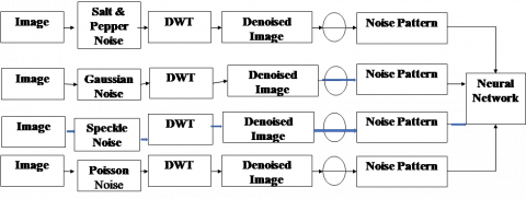
Figure 1. Designed system for noise pattern generation and image filtering using that information
The challenge with noise cancellation is that because noise is a random signal, it cannot be predicted or expressed mathematically. The goal of this work with filtering is to identify noise patterns so that the proper filtering technique can be utilized based on the nature of the noise. As a result, every type of noise filtration achieves standard results. Increasing the amount of noise in the training.
The survey on image denoising methods [3] has enriched the classification of denoising methods that were employed near or later past. The denoising methods are categorized in spatial and transfer domains. Spatial filtering in its non-linear approach defines the bandwidth of filters at lower frequencies subjected to the argument that artifacts or noise occur possess higher domain. These non-linear filters are specifically employed for the salt & pepper and speckle noise. The linear filters for additive noise like Gaussian operate on the same phenomenon. The transform domain filtering technique is the combination of adaptive and non-adaptive types of filtering. The adaptive filtering is limited to the ICA technique that assumes the noise to be non-Gaussian thus valid for all types of noise. The ICA samples the images in form of components independent of each other. Application of the shrinkage scheme [4] attempts to minimize the noise of ICA components andBayer filter mosaic [5] is the overhead computation to enhance the performance of ICA. Shawetangi Kala instead of ICA used Fast ICA [6] with Bayer filter for denoising. Sukhatme and Shukla (2012) [7] showed that ICA performs better than the simple non-adaptive approach method, however; the computation cost and relative assumptions are factors that check the performance measure here. The non-adaptive methods are generally wavelet methods that allow filtering of individual wavelets. The performance of wavelets is generally scaled in the number of wavelets formed and the value of threshold selected for filtering. The shrinking methods, Visu shrink and Sure shrink by Ruikar and Doye tends to minimize median and mean square error in wavelets respectively [8]. Many schemes exist that enhance the performance of wavelets yet its performance over ICA and problems related to ICA are yet a matter of discussion.
Noise classification can be done using its statistical features [9] as the noise affects the image in different ways. The image is first filtered using a non-linear spatial filter and the clean image is subtracted from the noisy image to get noise. Another approach used simple image filters and statistical and/or histogram-based features for noise classification in images [10]. Skewness and Kurtosis values of noise in another method were trained with NN for noise classification [11]. The authors did restrict their research only to the amount and type of noises available in a single image. Pipariya and Agrawal (2014) [12] proposed fuzzy logic approach for noise classification that draws their conclusion based on skewness and kurtosis values of noise. This approach holds good for noise patterns but the filtering through nominal filtering techniques has limited efficiency. Thus, the cleaned images have considerable noise and on subtraction with noisy images, the epochs of noise may get canceled rendering insufficient information of noise element. Not much literature is available on noise pattern classification and perhaps is an overlooked subject. Further employment of noise filters based on these patterns is a far cry [1].
In this paper, noise pattern information is exploited in the selection of filters for noise filtration in an image. The noise classification is subjected to the availability of noise patterns generated from filtered images and noisy images.
We can categorizse and denoise not only a certain form of noise but also mixed sorts of noise for real-time need in experiments. Because each form of noise has its unique features, it is difficult for a single filter to function for all types of noise. In medical images, picture clarity is critical; to improve PSNR and structural similarity, we categorized noise, making filtering more suitable. Two types of networks are used in our strategy. One is used to categorize the picture noise type, while the other does denoising depending on the first's classification result. With these efforts, our system can automatically denoise single or mixed forms of noise.
The results of our experiments suggest that our classification and denoising networks can produce significant PSNR and SSIM values than existing approaches.
2.1 The problem
The problem with noise cancellation is that noise is a random signal that cannot be defined in advance, nor could be formulated with any equation. Thus, the filtration of noise by any method possesses standard achievements. The task of noise scaling and pattern formation is supervised. Some scholars may claim that noise structure is only a byproduct of their algorithm's effectiveness, however this knowledge aids in the development of an efficient noise cancellation system. Because the process of capturing and processing medical pictures is almost equal in recurrence, noise (of any sort) in such a circumstance would have comparable amplitude and frequency attributes. Our information is crucial in this study because it allows us to build a fictitious noise pattern and pick filters for second-stage processing based on it. The globalization of computer vision applications has prompted the migration of noise from images and many methods are proposed over the years.
2.2 The proposed solution
Multiwavelets are wavelets with quite a lot of scaling functions and they offer parallel, orthogonality, evenness, and short support, which is not possible with common wavelets.
The main focus of this research is the selection of suitable filters based on the type of noise. As the noise is random, additive, or multiplicative, a single filter (linear or non-linear) cannot hold good responses for all three types of classified noises. The proposed system projects two-stage filtering of medical images.
I. The first stage of filtering through DWT eradicates most of the noise from the image. This image when mathematically differentiated with noisy image, the noise pattern is received.
II. This noise pattern information is the channel that mounts the fuzzy implementation of filters for second stage filtering. The pattern of noise classifies its type that is further enhanced through the repeated iterations performed using a standard classifier (Neural Network). The second stage of filtering exploits this information and the proposed system automatically assigns the relevant filter to dismantle that particular type of noise.
The organization of the paper is as follows: in section I, a formal introduction and related literature to support the cause of this research are present. In the second section, the proposed methodology illustrates the architecture of the system formulated in this paper. The subsections of section 2 are the mathematical descriptions of algorithms and tools acquired in this research. Section 3 illustrates the experimental setup for testing and evaluation parameters. Section 4 has the results of the proposed method and their description. Finally, the paper is ended with a conclusion in section 5.
The medical images are considered in the domain of three noises. The description is depicted in the above section. For the sake of this experimentation, the three noises are mixed virtually in images randomly. A single noise is considered in every image and two categories are divided, one for testing and another for experimentation. In the first phase, the noise is filtered with Discrete Wavelet Transform. The images are segmented into wavelets and soft-thresholding clips of the irregular artifact peaks. The filtered wavelets are reconstructed and the filtered image is given as output. This output image when subtracted with noisy image, a noise pattern is achieved (Figure 1). This noise pattern for all three types of images is collected and Neural Network classifies this pattern based on a given set of repeated tests. Once the system is trained, the experimental input images are repeated with these steps and a neural network based on its training classifies the noise in the image. Based on this, the Fuzzy based Weiner filter (for Gaussian noise) or Median filter (for speckle and salt & pepper noise) are selected for filtration. The main advantage of the proposed algorithm is:
Spatial domain filters are useful for noise reduction because they boost signal strength while reducing visual distortion. The restoration of a salt and pepper impulse noise-corrupted picture using an adaptive fuzzy median filter, which is particularly successful at eliminating extremely impulsive noise. To replace the noisy pixel, we first estimate the noise level using fussy set theory, then process the damaged pixel or increase the size of the filtering window, and finally acquire the suitable median value. The suggested filter has the advantages of being simple and requiring no prior knowledge of the input picture.
Several distinct picture-enhancing issues were used to test the capacity of our filtering methodology. The suggested approach performs well not only for photos with low percentages of impulse noise but also for pictures with greater percentages of impulse noise.
For estimation of II nd order derivatives by the Wiener filter, we developed an adaptive wiener filtering technique. In terms of peak-to-peak SNR, the resultant Wiener filter improves by roughly 1dB in experiments (PSNR). Furthermore, the perceptual improvement is considerable in that the irritating boundary noise, which is typical with typical Wiener filters, has been significantly reduced.
3.1 Discreet Wavelet Transform
Suppose an image x (Given by $x_{i j}, i=1,2 \ldots$ and $j=1,2 \ldots$) is a vector of $m \times n$ pixels corrupted due to any noise. Let $n_{i j}$ is the noise added by the system then the resultant image for experimentation will be given by
$y_{i j}=x_{i j}+n_{i j}$ (2)
The denoising methods attempt to locate information of x from image y in constraints of minimum means square error (MSE). The wavelet coefficients of Eq. (2) can be illustrated using a two-dimensional wavelet (W)
$X=W x, Y=W y, Z=W z$ (3)
The wavelet distribution of the input image has high-frequency Detailed Coefficients (DC) and low-frequency Approximate Coefficients (AC). The DC in the case of the image is a combined term of 3 points i.e. horizontal details, vertical details, and diagonal details. Figure 2 represents the illustrative block diagram of DWT format.
The image of Eq. (2) can be written in their wavelet transforms as [13]
$Y=X+N$ (4)
This Y as the input of wavelet (Figure 2) first segments the rows in the first level. In the second level of wavelets, columns are filtered out. The sub-sampling of the image results in four outputs.
Figure 2. Block representation of 2-Level DWT process
3.2 Soft thresholding
Thresholding in analytic form is expressed as:
$y=\operatorname{sign}(x)(|x|-T)$ (5)
The level of thresholds is subjected to thresholding criteria based on minimizing the average squared error
$\arg \min \left[\frac{1}{N} \sum_{i}\left(\hat{Y}_{i}-X_{i}\right)^{2}\right]$ (6)
Here, $\hat{Y}_{i}$ and $X_{i}$ represent the detailed threshold coefficients of the noisy and original image respectively.
The images after thresholding are reconstructed to original forms using inverse wavelet transform $W^{-1}$.
The SNR and MSE of experimental inputs in the results section support this conclusion. However, the outputs of DWT are clean enough to generate the noise pattern in the image. Let K represents the noise pattern for any specific noise
$s_{i j}=x_{i j}+k_{i j}$ (7)
Here, the noise $k_{i j}$ is considered instead of $n_{i j}$ as soft threshold filtering in wavelet transform filtered the input image $x_{i j}$, thus $n_{i j} \gg k_{i j} .$ Being $k_{i j}$ very small, and to classify the noise, this term is neglected from Eq. (7). Also, $s_{i j}$ can be considered as the original $x_{i j}\left(s_{i j} \sim x_{i j}\right)$, hence noise pattern can be obtained via subtracting Eq. (7) from Eq. (2):
$y_{i j}-x_{i j}=n_{i j}$ (8)
The value of $n_{i j}$ is processed through neural network for all the test signals to classify it among the all three categories of noise considered in this research.
3.3 Neural network
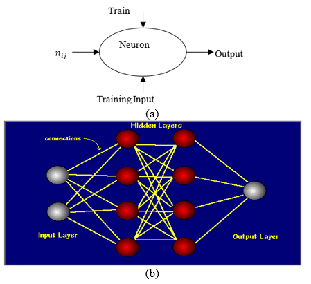
McCulloch and Pits proposed a binary threshold unit as a computational model for artificial neurons. The ANN is the duplication of an animal's central point nervous organism deliberately designed to meet the assistance of machine learning for pattern recognition. The neural network is a three-layer demonstration as shown in Figure 3 that diverts the input and progression it to generate output. Being user needy for its design ANN has no single depiction. In this mode, the neurons are trained to fire in an exacting manner. In case if input pattern does not bear a resemblance to the trained list of patterns, dismissal rules take the resolution of firing or holding the inputs.
In an explicit circumstance, BPNN's output matches Bayesian Posterior Probabilities. Statistical of samples (m) is represented in an adequate way to order prospect samples in the methodology developed for W number of weights and N number of nodes.
$m \geq O\left(\frac{W}{\epsilon} \log \frac{N}{\epsilon}\right)$ (9)
Figure 3. (a) Representation of Single Neuron (b) Neural Network with 2 Hidden Layers [14]
We are utilizing a feed-forward neural network, which processes signals in just one direction, from input to output. There are no feedback loops set up at any layer, and the output does not affect the same layer. This design is used in the majority of pattern recognition investigations. To create the adequate response of input signals, the teaching method of a neural network gathers data from an external source (supervised learning). Feed-forward neural networks are trained using Back Propagation Neural Networks (BPNN). In feature space, it produces complex classification boundaries. In some cases, the output of BPNN resembles Bayesian Posterior Probabilities. These requirements, as well as the choice of parameters such as training dataset, hidden layer nodes, and activation functions, are required to ensure low error performance for a specific collection of features.
3.4 Adaptive Weiner Filter
The images with Gaussian noise are filtered through the Fuzzy Weiner filter. Along with the statistical and time-invariant properties of the wiener filter, the overhead computation of fuzzy constantly modifies the filter coefficients through the autocorrelation process in constraints of noise [15]. As the median filter considers the additive noise in its problem domain, images with Gaussian noise are filtered through this algorithm [16]. The filter mean value “g” is convoluted in Eq. (7) to generate output response $\hat{s}(t)$
$\hat{s}(t)=g * x_{i j}+k_{i j}$ (10)
The error function is defined in terms of wiener delay and output of filter $s(t+\alpha)$
$e(t)=s(t+\alpha)-\hat{s}(t)$ (11)
The mean square error of the wiener output is
$\mu=\frac{1}{N M} \sum_{i, j \in k} y(i, j)$ (12)
Wiener filter derives the standard deviation and the mean for a given input image. Also, an assumption is made as zero mean and variance of noise and also non-correlation with an image. Based on these the mean $(\mu)$ and variance $(\sigma)$ are:
$\mu=\frac{1}{N M} \sum_{i, j \in k} y(i, j)$ (13)
$\sigma^{2}=\frac{1}{N M} \sum_{i, j \in k} y^{2}(i, j)-\mu^{2}$ (14)
The pixel-wise filtering of Wiener filter is thus referred from
$\hat{x}(i, j)=\mu+\frac{\sigma^{2}-\sigma_{n}^{2}}{\sigma^{2}}(y(i, j)-\mu)$ (15)
3.5 Fuzzy median filter
The median filter is a non-linear technique that preserves the edges and approximates the information of nearby pixels to overwrite pixels having abrupt values. The description of the median filter along with fuzzy implementation is well documented [17]. A 3×3 window is selected to filter the image $S_{i j}$ and pixels are arranged in ascending order from $a_{11}$ to $a_{33}$. The value of the pixel under consideration is tested in the range from minimum to maximum and also from 0 to 255. If the pixel satisfies these two conditions, it is assumed as clean. A fuzzy membership function based on the correction factor is employed for fuzzification and modification of values [18].
3.6 Proposed methods
The operation of filtering is segmented in two phases as required by Neural Network. The first phase is the learning of neural networks and the second is the testing phase.
The insertion of noise into the input data of a neural network during training is widely recognized. In some cases, this can result in large gains in generalization performance. Because training samples change all the time, adding noise makes the network less able to memorize them, resulting in smaller network weights and a more robust network with lower generalization error.
The noise makes it appear as if fresh samples are being drawn again from the field in the area of existing samples, softening the input space's structure. This reduction may make it easier for the network to function the mapping, resulting in easier and quicker learning.
DWT can save both the frequency and position of feature maps, which might be useful for maintaining detailed texture. In the expanding subnetwork, inverse wavelet transformations (IWT) are used to up sample low-resolution feature maps to high-resolution feature maps. In Denoising, wavelet analysis is a quick and effective way to detect different types of noise. ANN's capability in categorization may also be observed.
Data Collection- In terms of experimental data, collecting a varied range of data samples is usually a difficult challenge in medical image analysis. Furthermore, none of the existing datasets include a compilation of images gathered using various medical imaging modalities. However, a large number of training data samples are required to generalize the performance of any deep approach over a large data space. To solve this incongruent situation, our study gathered massive picture samples from many sources; the final dataset is made up of over 4500 images from 875 patients. Where 3600 samples were used for model training and the rest of the 20 percent data used for performance evaluation.
Training Section
In the training phase, the NN is fed with a pattern of noise. The three noises are fed to NN and the hidden layers draw an automatic array to classify them based on statistical properties. The noise pattern in this research is a simple term to refer to statistical noise.
A salt & pepper noise is added to the image to make it noisy. The Discreet Wavelet Transform breaks the image into several wavelets and the soft thresholding technique cleans the unconcerned epochs from the image. The inverse wavelet transform reconstructs the image in time-domain analysis. When this image is differentiated from the noisy image, the noise pattern for salt and pepper type of noise is generated. This noise pattern is fed to the neural network for classification. For Gaussian noise and Speckle noise above process is repeated and fed to the same neural network. The NN thus now has all the three noises and its internal structure knows the patterns that can recognize the type of noise in test input.
Testing Phase
The testing phase is the mixing of noise with an unknown noise (Anyone from the noise referenced in this research). The description of testing is well defined in the system model and Figure 4. The NN classifies the given noise and the system configures the respective filter based on it.
Figure 4. Training phase of neural network
3.7 Evaluation parameters
PSNR
PSNR is the ratio among the upper limit possible power of a signal and the power of undignified noise that influence the fidelity of its illustration.
The PSNR block calculates the peak signal-to-noise ratio between two pictures in decibels. This ratio is used to compare the quality of the original and a noisy picture. The better the quality of the compressed or reconstructed image, the greater the PSNR [16, 19].
Since a lot of signals contain a very extensive dynamic range, PSNR is more often than not articulated in expressions of the logarithmic decibel (dB) scale.
$P S N R=10 \lg \left(\frac{255^{2}}{E}\right) d B$ (16)
where, E is MSE, $f(i, j)$ is the pixel value of unique image $f^{\prime}(i, j)$ of the watermarked picture and its logarithmic unit is dB given by formula:
$E=\frac{1}{M \times N} \sum_{i=1}^{N} \sum_{j=1}^{M}\left[\left(f(i, j)-f^{\prime}(i, j)\right]^{2}\right.$ (17)
WPSNR
The weighted PSNR (WPSNR) has been distinct as an annex of the conformist PSNR. It weights each one of the expressions of PSNR by confined bustle factor (correlated to the local variance). The PSNR is not enough to measure even & texture. The solution of this problem is using weighted PSNR.
$W P S N R=10 \log \frac{\left(L_{\max ^{2}}\right)}{(M S E * N V F)^{2}}$ (18)
where, $N V F=\frac{1}{1+\theta \sigma_{x}^{2}(i, j)}, \theta=\frac{D}{\sigma_{x \max }^{2}}$.
where, $\sigma_{x \max }^{2}$ is the maximum local variance of a given image and $D \in[50,150]$ is a resolute factor.
Noise is classified according to its qualities. The NN is fed a noise pattern during the training phase. The three sounds are input into NN, which creates an automated array based on statistical features to categorise them. The word "noise pattern" is used in this study to refer to statistical noise. The reference document [20] is included for filterization decision; we followed it since it claims that the median filter delivers the best results for Poisson and Salt & Pepper noise. For Gaussian and Speckle Noise, the Weiner filter outperforms all other filters.
Database Collection: we tested our algorithm in four different ovarian images suffered from PCOS. We experiment that the test images have given away some development in most of the parameters in deliberation (PSNR, MSE, and WPSNR for various noise types). The selection of the second stage filter is powered by a noise pattern generated from the neural network.
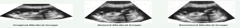
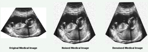
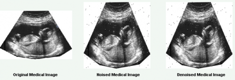
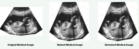
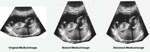
Results. IMAGE 1: Ultrasound image taken from reference [21].
Figure 5. Salt & Pepper noise effect
Figure 6. Gaussian noise effect
Figure 7. Speckle noise effect
Figure 8. Poisson noise effect
Figure 9. DWT enhanced image of Salt and pepper (a), Gaussian noise (b)
Figure 10. DWT enhanced image of Speckle noise (a), Poisson noise (b)
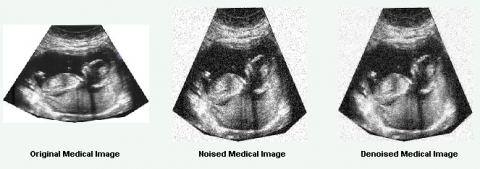
IMAGE 2: Ultrasound image taken from reference [21].
Figure 11. Salt & Pepper noise effect
Figure 12. Gaussian noise effect
Figure 13. Speckle noise effect
Figure 14. Poisson noise effect
Table 1. Comparison of new PSNR, MSE and WPSNR with the old values for Image 1
|
Image 1 |
Salt & Pepper |
Gaussian |
Speckle |
Poisson |
|
Proposed PSNR |
34.25 |
34.26 |
34 |
34.05 |
|
PSNR [22] |
33.98 |
31.57 |
33.44 |
33.32 |
|
Proposed MSE |
24.41 |
24.36 |
25.86 |
25.56 |
|
MSE [22] |
25.96 |
45.29 |
29.43 |
30.23 |
|
Proposed WPSNR |
34.93 |
32.09 |
34.83 |
35.03 |
|
WPSNR [22] |
32.85 |
32.65 |
32.56 |
32.67 |
Table 2. Percentage improvement or degradation in PSNR, MSE and WPSNR for Image 1
|
Image 1 |
Salt & Pepper |
Gaussian |
Speckle |
Poisson |
|
PSNR % Improvement or Degradation |
0.8 |
8.5 |
1.7 |
2.2 |
|
MSE Improvement or Degradation |
6.0 |
46.2 |
12.1 |
15.4 |
|
WPSNR Improvement or Degradation |
5.95 |
0.77 |
15.4 |
6.74 |
Table 3. Comparison of new PSNR, MSE and WPSNR with the old values for Image 2
|
Image 2 |
Salt & Pepper |
Gaussian |
Speckle |
Poisson |
|
Proposed PSNR |
31.71 |
29.81 |
29.42 |
30.81 |
|
PSNR [22] |
31.83 |
28.15 |
29.16 |
30.12 |
|
Proposed MSE |
43.81 |
67.85 |
74.18 |
53.84 |
|
MSE [22] |
42.59 |
91.43 |
78.81 |
63.2 |
|
Proposed WPSNR |
31.75 |
29.26 |
30.15 |
31.6 |
|
WPSNR [22] |
29.96 |
28.69 |
28.46 |
29.3 |
Table 4. Percentage improvement or degradation MSE and WPSNR for Image 2
|
Image 1 |
Salt & Pepper |
Gaussian |
Speckle |
Poisson |
|
PSNR % Improvement or Degradation |
-0.4 |
5.9 |
0.9 |
2.3 |
|
MSE Improvement or Degradation |
-2.9 |
25.8 |
5.9 |
14.8 |
|
WPSNR Improvement or Degradation |
5.64 |
1.95 |
5.61 |
7.28 |
4.1 Comparison with existing work
Comparison with other existing methods like anisotropic filter, NLM filter, PNLM filter is also reflected that in PSNR proposed method performs better as shown in Table 5. In terms of structure similarity also slight improvement is shown by the proposed method as it reflects in Table 6. For time calculations it is shown in Table 7 those other methods perform better because they are performing denoising process only but our proposed method will perform double-stage filtering and classifying noise pattern as well. The difference of time is not much, we will try to reduce this in future experiments.
Table 5. Comparison in terms of PSNR [19]
|
Image |
Anisotropic Filter method |
NLM Method |
PNLM Method |
Proposed method |
|
|
|
Noise Std. dev. |
PSNR |
PSNR |
PSNR |
PSNR |
|
Image 1 |
10 |
29.73 |
34.57 |
34.85 |
35.32 |
|
Image 2 |
10 |
26.21 |
3173 |
31.69 |
34.3 |
|
Image 3 |
10 |
25.72 |
31.51 |
31.49 |
33.85 |
|
Image 4 |
10 |
28.16 |
33 |
33.08 |
33.89 |
Table 6. Comparison in terms of SSIM [19]
|
Image |
Anisotropic Filter method |
NLM Method |
PNLM Method |
Proposed method |
|
Image 1 |
0.8513 |
0.8993 |
0.8993 |
0.9123 |
|
Image 2 |
0.8033 |
0.8998 |
0.8998 |
0.8124 |
|
Image 3 |
0.8995 |
0.9952 |
0.9952 |
0.8994 |
|
Image 4 |
0.8124 |
0.8652 |
0.8652 |
0.9654 |
Table 7. Comparison in terms of TIME [23]
|
Method |
Time in sconds |
% Reduction in time |
|
Anisotropic Filter method |
53 |
37.73 |
|
NLM Method |
368 |
82.08 |
|
PNLM Method |
77 |
71.93 |
|
Proposed method |
76 |
71.14 |
Enhance the denoising execution of spatial space averaging sort channels. The standard spatial channels, for example, Anisotropic sifting, Bilateral separating, non-neighborhood implies separating, and Probabilistic non nearby means separating have been considered for experimentation. As the preprocessing channel is planned in the wavelet space, it gives a composite impact on enhancing the denoising execution of the given crossbreed strategy at high frequencies. Exploratory results demonstrate that the technique not just enhances the denoising execution as far as PSNR, SSIM, and visual presentation; additionally, it lessens the execution time required for denoising [24]. The resulted output shows four noise domains are shown in Figures 9 and 10, firstly DWT for various noise type (Salt & pepper, Gaussian, Speckle, and Poisson noise) for the standard variance of 0.02 and different values of PSNR, MSE, WPSNR, SSIM and Run time for different noise category are found as shown in Table 1 and Table 3. Table 1 and Table 2 shows that that image 1 has shown great improvement in MSE (nearly 46% improvement) as well as PSNR (nearly 9% improvement) when gaussian noise is to considered compare to the other noises. Other noises have also shown improvement. We also observed that WPSNR has degraded in all cases except gaussian noise. The structural similarity index seems to be improved in all cases. For image 3 gaussian noise has been well taken care of in reducing MSE and improving PSNR and SSIM as shown in Table 3 and Table 4. Reduction of WPSNR is seen in all the noise types. A better structural similarity improvement is seen for salt & pepper noise but showing a reduction in the other three parameters.
The resultant output images are then subsequently enhanced by passing them through the two filters. The output of four different noise salt & pepper, Gaussian noise, Speckle Noise & Poisson noise is shown for image 1 in Figure 4, Figure 5, Figure 6, Figure 7 and Figure 8 respectively in sequence fuzzy median filter and adaptive wiener filter. Same analysis will be carried out for Image 2 using four different noise and output shown in Figure 11, Figure 12, Figure 13, Figure 14 for four different noise, salt & pepper, Gaussian noise, Speckle noise & Poisson noise respectively [13].
The results indicate that high performance is achieved as MSE in using adaptive wiener and fuzzy median filters. The WPSNR in both MRI and ultrasound images also have comparative better values as shown in the Table 3 and 4. Figure 12 indicates that in Gaussian noise, the MSE for old methods is high while the proposed system was efficient to clip it at a great level. Nearly 30% improvement is seen in PSNR, whereas MSE has decreased to nearly 97% after double-stage filters. These improvements have helped to achieve better WPSNR between 29% to 40% improvement in various image type.
The attempt of dual-stage filtering images for the medical field is executed efficiently. The noise was analyzed with a focus on its ill effects in PCOS Images that can lead to the evaluation of diseases. Four different follicle images of UltraSound are used to test the systems. The noises used for evaluation are standard as they give their mere presence in almost every case of imaging. A comparative study of different noises is performed in different images. The MSE, PNSR, and WPSNR were used to evaluate the system. The noisy images after the first stage filtering did not possess a very good response to be considered as the effective solution. Also, the thresholding value and number of wavelets are chosen manually. The manual choice of wavelets can be justified to obtain the noise pattern; no need for an optimization algorithm in wavelets is required. The neural network for deriving noise pattern determines the type of noise and second stage filtering through adaptive wiener filter and fuzzy median filter independently reduces the mean square error in all three noises at a good proportion. The images with Gaussian noise cannot be filtered through a median filter hence fuzzy median filter is used. While performing the test on the system, a person may not have the information about the type of noise he is encountering, the system itself identifies the type of noise and cascades the respective filter against it. Apart from salt and pepper noise, Gaussian noise, speckle noise & Poisson noise have shown improvement to some extent but salt and pepper have stood apart from all the noises.
[1] Bhargava, S., Somkuwar, A. (2016). Estimation of noise removal techniques in medical imaging data—a review. Journal of Medical Imaging and Health Informatics, 6(4): 875-884. https://doi.org/10.1166/jmihi.2016.1797
[2] Verma, R., Ali, J. (2013). A comparative study of various types of image noise and efficient noise removal techniques. International Journal of Advanced Research in Computer Science and Software Engineering, 3(10): 617-622.
[3] Motwani, M.C., Gadiya, M.C., Motwani, R.C., Harris, F.C. (2004). Survey of image denoising techniques. In Proceedings of GSPX, 27: 27-30.
[4] Zhang, Q., Yin, H., Allinson, N.M. (2000). A simplified ICA based denoising method. In Neural Networks. Proceedings of the IEEE-INNS-ENNS International Joint Conference, 5: 479-482. https://doi.org/10.1109/IJCNN.2000.861515
[5] Kala, S., Sahu, R.K. (2012). ICA based Image denoising for single-sensor digital cameras. IOSR Journal of Engineering, 2(3): 446-450.
[6] Kala, S., Sahu R.K. (2013). FASTICA based denoising for single sensor digital cameras images. International Journal of Electronics and Computer Science Engineering, 2(1): 1026-1033.
[7] Sukhatme, N., Shukla, S. (2012). Independent component analysis based denoising of magnetic resonance images. International Journal of Computer Applications, 54(2): 13-18.
[8] Ruikar, S.D., Doye, D.D. (2011). Wavelet based image denoising technique. International Journal of Advanced Computer Science and Applications, 2(3): 49-53. https://doi.org/10.14569/IJACSA.2011.020309
[9] Subashini, P., Bharathi, P.T. (2011). Automatic noise identification in images using statistical features. International Journal for Computer Science and Technology, 2(3): 467-471.
[10] Chen, Y., Das, M. (2007). An automated technique for image noise identification using a simple pattern classification approach. In 2007 50th Midwest Symposium on Circuits and Systems, pp. 819-822. https://doi.org/10.1109/MWSCAS.2007.4488699
[11] Santhanam, T., Radhika, S. (2011). Probabilistic neural network–a better solution for noise classification. Journal of Theoretical and Applied Information Technology, 27(1): 39-42.
[12] Pipariya, T., Agrawal, S. (2014). Statistical moments and fuzzy logic based classification of noise present in digital images. International Journal of Advanced Research in Computer and Communication Engineering, 3(7): 7453-7456.
[13] Bhargava, S., Somkuwar, A. (2013). Hybrid filters based denoising of medical images using adaptive wavelet thresholding algorithm. International Journal of Computer Applications, 83(3): 18-23. https://doi.org/10.5120/14428-2572
[14] http://pages.cs.wisc.edu/~bolo/shipyard/neural/local.html, accessed on June 17, 2021.
[15] Jin, F., Fieguth, P., Winger, L., Jernigan, E. (2003). Adaptive Wiener filtering of noisy images and image sequences. In Proceedings 2003 International Conference on Image Processing (Cat. No. 03CH37429), 3: III-349. https://doi.org/10.1109/ICIP.2003.1247253
[16] Nandan, D., Kanungo, J., Mahajan, A. (2018). An error-efficient Gaussian filter for image processing by using the expanded operand decomposition logarithm multiplication. Journal of Ambient Intelligence and Humanized Computing, 1-8. https://doi.org/10.1007/s12652-018-0933-x
[17] Deshpande, B., Verma, H.K., Deshpande, P. (2012). Fuzzy based median filtering for removal of salt-and-pepper noise. International Journal of Soft Computing and Engineering (IJSCE), 2(3): 76-80.
[18] Zhou, Y., Tang, Q., Jin, W. (2008). Adaptive fuzzy median filter for images corrupted by impulse noise. 2008 Congress on Image and Signal Processing, pp. 265-269. https://doi.org/10.1109/CISP.2008.231
[19] Avinash, G.P., Kumar, P.R., Adiraju, R.V., Nandan, D. (2021). A study on low-frequency signal processing with improved signal-to-noise ratio. In Proceedings of International Conference on Recent Trends in Machine Learning, IoT, Smart Cities and Applications, pp. 857-864. https://doi.org/10.1007/978-981-15-7234-0_80
[20] Kumar, N., Nachamai, M. (2017). Noise Removal and Filtering Techniques used in Medical Images, Oriental Journal of Computer Science & Technology, 10(1): 103-113. https://doi.org/http://dx.doi.org/10.13005/ojcst/10.01.14
[21] www.ablesw.com, accessed on June 17, 2021.
[22] Baselice, F., Ferraioli, G., Pascazio, V., Schirinzi, G. (2017). Enhanced Wiener Filter for Ultrasound image denoising. In: Eskola H., Väisänen O., Viik J., Hyttinen J. (eds) EMBEC & NBC 2017. IFMBE Proceedings, vol 65: 65-68. Springer, Singapore, https://doi.org/10.1007/978-981-10-5122-7_17
[23] Gopalan, B. Chilambuchelvan, A., Vijayan, S., Gowrison, G. (2015). Performance improvement of average based spatial filters through multilevel preprocessing using wavelets. IEEE Signal Processing Letters, 22(10): 1698-1702. https://doi.org/10.1109/LSP.2015.2426432
[24] Goel, A., Bhujade, R.K. (2020). A functional review, analysis and comparison of position permutation based image encryption techniques. International Journal of Emerging Technology and Advanced Engineering, 10(7): 97-99.