Shilpi Aggarwal* | Madhulika Bhatia | Rosy Madaan | Hari Mohan Pandey
© 2021 IIETA. This article is published by IIETA and is licensed under the CC BY 4.0 license (http://creativecommons.org/licenses/by/4.0/).
OPEN ACCESS
In today's time, our nature is fighting against many life-threatening problems which can even threaten the existence of life on the Earth. Pollution is one of the deadliest problems among them. It is caused primarily by means of air, water and land but air pollution is the most severe and dreadful among them. It is caused by introduction of toxic substances like oxides of Sulphur, nitrogen and carbon into the atmosphere making it unfit for living beings. Along with humans, plants have also become a victim to it, and this fact is mostly ignored. A model has been designed to predict the effect of pollution on plants. Image samples of 5 Indian oxygen rich plants namely Ocimum Tenuiflorum, Sansevieria Trifasciata, Chlorophytum Comosum, and Azadirachta Indica have been taken for analysis and various properties like shape, color, corners and texture of the plants were considered from these input RGB images. As a consequence of these properties and the pollution index value, certain calculations have been performed and the results are compared with the threshold values. Based on the range in which the calculated results lie, the plants will be categorized into a category which depicts the severity level of pollution in the environment. After applying the model on the images, a dataset was prepared and SVM classification model has been trained on it which predict with an accuracy of 85%. It has been presented in the form of an interactive user interface to predict the effect of pollution on plants. Plants are an integral part of nature and should not be ignored.
pollution, plants, prediction, classification, air quality index, GUI
The presence of hazardous elements into the environment is known as pollution. Air, water and land pollution are the three prominent categories of pollution, air pollution being the most severe and dangerous among them. Burning of fossil fuels is the primary cause of air pollution. It includes the smoke from industries, automobiles and other machines. Burning crackers and fire accidents are also among the contributing factors. The pollutants comprise of particulate matter and a number of gases. Sulphur dioxide, nitrogen dioxide, carbon dioxide, carbon monoxide etc. are regarded as highly toxic gases. These polluting substances have pathetic consequences on human health and plant life. They lead to global warming which in turn triggers the melting of glaciers leading to floods, soil erosion, droughts, fires, loss of wildlife and as a result, the complete ecological balance gets disturbed.
The quality of air can be checked by the Air quality index (AQI) value. It indicates the degree of pollution in the air. The higher the AQI value, the greater the level of air pollution and the greater the health concern. It depends upon the concentration of various pollutants like Sulphur dioxide (SO2), nitrogen dioxide (NO2), particulate matter etc. The algorithm to calculate AQI is defined by the Indian National Air Quality Standards (INAQS) [1].
There are around 390,800 different plant species surviving on earth. According to a botanist, about 21 percent of the total plant species on earth are on the path of extinction [2]. Amidst so much deforestation, sustaining the plant species is very difficult but the need of the hour. In order to achieve this goal, recognition and classification of endangered species is indispensable. Different researchers have proposed several algorithms for the recognition of plants. These algorithms include the techniques like deep learning [3, 4] and machine learning [5, 6] and they are widely used for the identification process.
During the 18th century, some classification schemes for plants were developed by Carolus Linnaeus [7]. There are many other classification techniques which are used to classify objects. The algorithms like Naïve Bayes, Support Vector Machine, K Nearest Neighbor along with the hybrid approaches were also applied by many researchers [8-11].
This paper starts the sequence with an introduction, continuing with the related work. Next section speaks about the material and methods required to implement the research. Third section explains the proposed model in detail. In continuation to this section, results obtained after implementation of the model and the graphical user interface have been discussed which show the effect of pollution on plants. Then the final section gives the conclusion of the paper.
As per a report published by the World Health Organization, the average life span of humans has got diminished by one year because of air pollution [12]. Human beings are suffering from life threatening diseases like liver infections, respiratory problems, skin diseases, cancers etc. just because of pollution. In fact, it is creating a detrimental impact on plants also. Numerous investigations have proved that the morphological properties of plants are badly impacted because of exposure to pollution. It has been deliberated and examined by several researchers that plants are acquiring morphological, structural as well as textural changes in the long term [13-15]. Sulphur dioxide is one of the most hazardous pollutants present in the air. It admits the leaves through stomata and leads to acute and chronic injuries. Exposure to high levels of Sulphur dioxide is responsible for acute injuries and its prolonged exposure causes chronic injuries. These injuries create physiological imbalance in plants and hinder their growth. This impact could also be seen visually in the form of chlorosis and red blotches on the leaves [16]. The pollutants present in the air create a severe disturbance in the process of photosynthesis. They retard the process of food preparation and deteriorates the all-round development of plants [17]. Giri et al. found that the presence of smoke and aerosol in the air leads to reduced levels of chlorophyll in leaves [18].
Shilpi et al. projected the algorithm to demonstrate the effect of pollution by the SSIM value with the pollution index. From the analysis and plotted graphs, it has shown a change in Indian plants due to the effect of air pollutants by using the Structural Similarity Intensity Measure (SSIM). As a result, it has been well proved that with an increase in SSIM value corresponding to a particular pollution index, image quality gets degraded [19].
Aggarwal et al. proposed an optimized model for plant recognition which is implemented using Keras library. Image samples of some oxygen rich Indian plants which also possess antioxidant properties were picked up for analysis. One Hot encoding was also applied on the dataset to optimize the model. It used sequential model with Keras and gave the accuracy of 96.7% with the testing dataset [20].
Aggarwal et al. proposes an algorithm to classify the leaves on the basis of shape features like area, perimeter, centroid and bounding box. On the basis of these collected features, leaves were classified through visualization method. The idea behind this research was to classify and categorize the plant species so as to ease their identification. This will help in achieving a dual goal by saving the endangered species from becoming extinct and reducing global warming by protecting air purifying plants [21].
Categorization [22] of species of flora can be carried out on the ground of features such as shape, color, texture etc. Denis Tsygankov proposed a method to calculate features on the basis of graphical methods. The accuracy for this method comes out to be 78.34 with Centroid Contour Distance Curve and 58.08% with Random Forest Classifier [23]. Du et al. applies MMC classifier to classify leaves on the basis of shape features [24]. Zhang and Chau [25] used semi supervised locally linear embedding technique with the combination of K-NN classifier. Chaki et al. applied hierarchical approach to categorize the leaves [26]. The fusion of shape [27], color [28], and texture were also applied in automatic classification [29, 30]. Palanisamy works on K means clustering to categorize leaf images drawn from color features [31]. Saleem uses several classifiers on Flavia dataset and KNN was found to be better than all [32]. Aggarwal et al. has done the classification of oxygen rich plants. All the processing of the plant samples was performed on MATLAB 2019a and features were extracted by applying the grab cut and gray level co-occurrence matrix. Then the collected data features are fed in different classification models like multi-layer perceptron, support vector machine and Random Forest. Finally, the Random Forest classification model is used to classify oxygen rich plants based on morphological properties which gives better results [33].
All the processing of the plant image samples can be done through the technique called image processing which processes the images digitally. Images f(x,y) where x and y are the image coordinates are processed on the basis of nature and type of the problem. Digital image processing has wide applications in numerous areas like medical imaging [34-37], pattern recognition, biotechnology, computer vision and many others.
The work done by all the researchers is highly appreciable. The investigation is being done on the available datasets. The effect of air pollution on the flora has been detected by some chemical experiments done by various scientists in their chemical laboratories. On the basis of some anomalies found, effort has been made to investigate and lookout the changes in plants caused by the pollutants present in air. This work has been carried out through the process of digital image processing. Samples were collected in the form of images and a dataset was created for the proposed research. Along with these image samples, the air quality index was also considered as an input for the analysis. After the compilation of the dataset, all the samples were processed using MATLAB 2020 b. Features were extracted from the image samples and the steps mentioned in algorithm 1 were applied. Then a classification model has been trained on this dataset which can predict the level of contamination.
Contamination level has been classified into five main categories namely, Satisfactorily polluted, Moderately polluted, Poorly polluted, Very poorly polluted and Severely polluted. The prepared dataset was also used to apply Naive Bayes, KNN, Trees, SVM and ensemble classifiers. Finally, SVM classifier provided the best results with the accuracy of 85%. Then, the model has been organized and presented through a graphical user interface (GUI). Inputs of GUI are the images of plant species (Ocimum Tenuiflorum, Sansevieria Trifasciata, Chlorophytum Comosum, Azadirachta Indica and Aloe Vera) and the pollution index of the respective day on which the image was captured. Then, the effect of pollution on the plant is calculated and displayed on the GUI. The objective of this research is very closely related to the health of our ecosystem to check the effect of air pollution on the wellbeing of plants.
3.1 Materials
Five Indian plant species of same age belonging to different categories were planted in different pots. The species used in this research are shown in Table 1 along with the common names and the scientific names. All the samples selected for the research were at the same stage and free from insects. For the analysis, 150 RGB images were captured through a 12.1 mega pixel digital camera. The resolution of the images captured was 4000 x 3000 pixels. These plant species have favorable properties with respect to the environment. Ocimum Tenuiflorum has antioxidant properties. Sansevieria Trifasciata inhales the carbon monoxide (CO) from the air. Chlorophytum Comosum purifies the air and also takes up the CO, formaldehyde (CH2O) and xylene (C8H10) from the atmosphere. Azadirachta Indica possesses medicinal properties. It is used to cure many liver infections, stomach infections etc. Aloe Vera is considered as the last species. It is an antioxidant as well as antibacterial plant which has a protecting action against the ultra violet rays. The air quality checker system which is positioned in Faridabad was used to record the pollution index for the respective days on which the samples were collected.
Table 1. Input plant species
|
Sample No. |
Scientific Names |
Common Names |
|
1 |
Ocimum Tenuiflorum |
Holy Basil |
|
2 |
Sansevieria Trifasciata |
Snake |
|
3 |
Chlorophytum Comosum |
Spider |
|
4 |
Azadirachta Indica |
Neem |
|
5 |
Aloe Vera |
Indian Aloe |
3.2 Air quality index
In order to rate the quality of the air, a standard known as air quality index is referred which represents the quality of air and the extent up to which it is polluted. The Air quality Index was evolved by United States Environmental Protection Agency (EPA) which is widely acceptable and comes up with the six categories namely Good, Satisfactory, Moderately Polluted, Poorly, Very poor and Severe. For the calculation of AQI there are mainly five major contaminates which includes Carbon Monoxide (CO), Nitrogen Dioxide (NO2), Particulate Matter (PM), Sulphur Dioxide (SO2), ground level ozone. The National Ambient Air Quality Standard (NAAQS) is being followed by the EPA for the respective pollutant to guard the public health. Greater is the value of AQI, poorer is the quality of air and it will be more harmful for us. Its formulation depends upon the concentration of various pollutants in the air like Sulphur dioxide, nitrogen dioxide, particulate matter etc. The Central Pollution Control Board of India has standardized certain ranges for the quality of the air. The range of pollution index for different categories is shown below in Table 2.
Table 2. Categories of different ranges of AQI
|
Good |
Satis factory |
Moderately polluted |
Poor |
Very Poor |
Severe |
|
(0-50) |
(51-100) |
(101-200) |
(201-300) |
(301-400) |
(> 401) |
From Table 2, we can see that air quality index of value greater than 401 is considered to be severe, while a value less than 50 is regarded as the best.
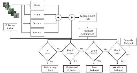
Foremost, it is very important to understand the impact of pollution on plants in different ways so as to design a prediction model which can predict the consequences of pollution accurately. The features considered from the input plant images are shape, color, texture and corners. First of all, the shape feature is evaluated and then a set of other properties like area, perimeter, major axis length and minor axis length are evaluated for each connected component in the binary image.
The model has been designed to identify and show the effect of pollutants on plants. The species for analysis were selected keeping in mind that they possess some air purifying or medicinal properties. Multiple features were extracted from the image samples and it was observed that morphological features like shape, color, texture, and corners got affected by air pollution. Polluted air contains harmful gases which create an adverse effect on plants. Researchers have already carried out multiple studies to find the effect of air contaminants on plants. They have performed several chemical experiments which show that plants are affected by contaminates present in the air.
The proposed model is designed to prepare a dataset from plant images and to predict the level of contamination. Categorization is completely based upon the contamination level and it is shown clearly in Figure 1. An algorithm has been formulated to get the desired output and accomplish the goal in the problem domain and it is elucidated in algorithm 1. The procedure for extracting features from the input image will be as per the following algorithm.
Algorithm 1
Input: (i) I(x,y): RGB input image belongings to one of the five categories.
(ii) PI: Pollution Index
Output: To calculate Pollution Effect (PE)
3.1 $\left(a, p, m_{i}, m_{o}\right) \leftarrow$Shape (I(x,y)).
3.2 $C \leftarrow$ Color (I(x,y)).
3.3 $\left(c, c_{o}, e, h\right) \leftarrow$Texture (I(x,y)).
3.4 l← Corner (I(x,y)).
4. Take the summation V of step 3.
$V=\sum a, p, m_{i}, m_{a}, C, c, c_{o}, e, h, l$
$M=\frac{\sum a, p, m_{i}, m_{a}, C, c, c_{o}, e, h, l}{P I}$
6.1 Evaluate the satisfactory threshold T1
$T 1=\frac{M}{\text { median of satisfactory } \operatorname{range}(l b, u b)}$
6.2 Evaluate the moderate threshold T2
$T 2=\frac{M}{\text { median of moderately polluted } \operatorname{range}(l b, u b)}$
6.3 Evaluate the poor threshold T3
$T 3=\frac{M}{\text { median of Poor Polluted range }(l b, u b)}$
6.4 Evaluate the very poor threshold T4.
$T 4=\frac{M}{\text { median of Very Poor range }(l b, u b)}$
7.1. If M>T1
Print ‘PE: Satisfactorily polluted’
7.2 Else If T1>M>T2
Print ‘PE: Moderately polluted’
7.3 Else If T2>M>T3
Print ‘PE: Poorly polluted’
7.4 Else If T3>M>T4
Print ‘PE: Very poor polluted’
7.5 Else
Print ‘PE: Severely Polluted’
8. End If.
9. End While loop.
End
Figure 1. Proposed model to show the pollution effect
|
Algorithm-1.1 Calculate Plant Shape Properties |
|
|
Input: I(x,y): RGB input image belonging to one of the five categories. Output: To calculate area (a), perimeter (p), minoraxislength (mi) and the majoraxislength (ma) |
|
|
|
Start |
|
|
While ($I_{\text {count }} \geq 0$) |
|
|
Convert the RGB values to CIE 1976 L*a*b* values. $I_{l a b} \leftarrow \operatorname{rgb} 2 \operatorname{lab}(I(x, y))$ |
|
|
Extract the foreground and background pixel $[$ foreground, background $] \leftarrow I_{\text {lab }}$ |
|
|
Compute the Super pixels from the image. |
|
|
Convert L*a*b*image to range [0, 1]. $I_{\text {range } 0,1} \leftarrow I_{l a b}$ |
|
|
Segmented image will be obtained by separating the foreground and background pixels using graph based segmentation. $I_{\text {seg }} \leftarrow$ graphcut $\left(I_{l a b}\right)$ |
|
|
Create the masked image. $I_{\text {mask }} \leftarrow$ graphcut $\left(I_{l a b}\right)$ |
|
|
$\left(a, p, m_{i}, m_{a}\right) \leftarrow I_{\text {seg }}$ |
|
|
End while loop |
|
|
End |
The shape feature is evaluated by the algorithm 1.1 and it is considered as a subroutine for evaluating shape. Initially the RGB input image is converted into L*a*b* color space. Then super pixels from the image are calculated. Depending upon the super pixels, the image is segmented by using the grab cut algorithm [38]. As a result, the binary image separates the foreground and background pixels. Then the properties like area (a), perimeter (p), minoraxislength (mi) and the majoraxislength (ma) are evaluated.
The color feature is extracted by algorithm 1.2. For the extraction of the color value, the green layer is extracted from the three color layers present in the RGB image. Then, median is calculated using equation 1which is given below.
$\operatorname{Med}(x)=\frac{x\left[\frac{n}{2}\right]+x\left[\frac{n+1}{2}\right]}{2} \quad$ if $n$ is even
$x\left[\frac{n+1}{2}\right] \quad \text { if } n \text { is odd }$ (1)
where, x acts the input array; n is the size of the array.
By summing all the median values, mean is calculated through the Eq. (2). The resulting value is the color value C of the associated image.
$C=\frac{\sum x}{n}$ (2)
where, x is the input array; n is the size of the array.
The texture features are evaluated on the basis of the gray tone of the image as given in algorithm 1.3. These gray tones are a part of the spatial pattern of the resolution cells which comprise of discrete values. For the calculation of textural features, the RGB image is converted into a grayscale image. Then theGrabCut algorithm [38] is applied to find the grey level co-occurrence matrix (GLCM). The Grabcut Algorithm is an optimized graphcut algorithm which combines texture and edge information. It has made of two improvements over graphcut mechanism i.e., “iterative estimation” and “incomplete labelling”. The basic steps in the algorithm includes segmentation followed by border matting in which the alpha values are computed in the narrow strip around the hard segmentation boundary.Then, the statistics like contrast c, correlation co, energy e, and homogeneity h are calculated.
|
Algorithm-1.2 Extract Plant Color Values |
|
|
Input: I(x,y): RGB input image belonging to one of the five categories. Output: Color value C |
|
|
|
Start |
|
|
While ($I_{\text {count }} \geq 0$) |
|
|
Extract the green layer from the three layers present in the RGB image. $I_{\text {green }} \leftarrow I_{\text {rgb }}$ |
|
|
Calculate the median of all the pixel values present in the green layer $\operatorname{Med}(x)=\left\{\begin{array}{l}\frac{x\left[\frac{n}{2}\right]+x\left[\frac{n+1}{2}\right]}{2} \text { if } n \text { is even } \\ \left.x \mid \frac{n+1}{2}\right] \quad \text { if } n \text { is odd }\end{array}\right.$ |
|
|
Calculate the mean for all the median values by equation 2. $C=\frac{\sum x}{n}$ |
|
|
End while loop |
|
|
End |
|
Algorithm-1.3 Calculate Plant Texture Properties |
|
|
Input: I(x,y): RGB input image belonging to one of the five categories. Output: To calculate contrast c, correlation co, energy e, homogeneity h |
|
|
|
Start |
|
|
While $\left(I_{\text {count }} \leq 0\right)$ |
|
|
$I_{G r a y} \leftarrow I_{r g b}$ |
|
|
$I_{\text {binary }} \leftarrow$ grabcut $\left(I_{\text {Gray }}\right) .$ |
|
|
glcm $\leftarrow$ gracomatrix(Ibinary) |
|
|
$\left(c, c_{o}, e, h\right) \leftarrow$ graycoprops(glcm) |
|
|
End while loop |
|
|
End |
|
Algorithm-1.4 Calculate Plant Corners |
|
|
Input I(x,y): RGB input image belongs to one of the five categories. Output: To calculate the length of corners l |
|
|
|
Start |
|
|
While ($I_{\text {count }} \geq 0$) |
|
|
$I_{\text {Gray }} \leftarrow I_{r g b}$ |
|
|
l $\leftarrow$ detectHarrisfeatures(IGray) |
|
|
End while loop |
|
|
End |
Corner feature is evaluated by implementing the algorithm 1.4. Corner points are the feature points that are detected in 2D grayscale image. These feature points are calculated by applying the Harris Stephens algorithm [39].
After evaluating all the features, summation is performed. Measurement M is calculated by applying the equation 3. The next step is threshold comparison. As each and every plant has its own capabilities to fight with pollution and external factors, the threshold value varies from plant to plant. As each and every plant has its own capabilities to fight with pollution and external factors, the threshold value varies from plant to plant. Here the threshold value of the plant is considered with respect to pollution index ranges given by Air Quality Standard followed by Central Pollution Control Board (CPCB). The threshold value was determined with the help of features calculated for a respective plant and the ranges given by the Air quality standard (AQI). Therefore, four threshold values are calculated with respect to each plant in the proposed model. The threshold values for all the four categories namely, Satisfactorily polluted, Moderately polluted, Poorly polluted and Very poorly polluted are denoted as $T_{1}, T_{2}, T_{3}, T_{4}$ respectively and they are calculated by the Eq. (4)-(7).
$M=\frac{\sum a, p, m_{i}, m_{a}, C, c, c_{o}, e, h, l}{P I}$ (3)
where, $a, p, m_{i}, m_{a}, C, c, c_{o}, e, h, l$ and $P I$ are area, perimeter, minoraxislength, majoraxislength, color value, contrast, correlation, energy, homogeneity, length of corner points, pollution index respectively.
The PI value is the pollution index for the day on which the image was captured. It is the AQI which was measured by the AQI checker system located in Faridabad. This system has been established by central pollution control board, India.
$T 1=\frac{M}{\text { median of satisfactory range }(l b, u b)}$ (4)
$T 2=\frac{M}{\text { median of moderately polluted range }(l b, u b)}$ (5)
$T 3=\frac{M}{\text { median of Poor Polluted } \operatorname{range}(l b, u b)}$ (6)
$T 4=\frac{M}{\text { median of Very Poor range }(l b, u b)}$ (7)
The measurement value M is compared with different threshold values. After comparison, the severity of the impact of pollution on the plant can be estimated into one of the categories on the basis of the range into which M lies. This outcome of the model is indicative of the pollution level.
4.1 Results and discussion
On the basis of the dataset prepared by implementing the above algorithms, a linear SVM classification model has been trained. The size of the dataset is 200 X 13. The dataset was partitioned into 80:20 ratio for training and testing data respectively. The dataset (to fit into my application) consists of RGB images having size of 3000X4000 pixels. Those images were collected for the 12 months continuously in all seasons to check the effect of pollution. In order to maintain the quality of the image, were captured through a 12.1 mega pixel digital camera. In future, this dataset can be used for any pollution-based application for researchers. While training the data, some specific features were selected for optimizing the results. 11 out of features were selected for this. While training the model, the prediction speed was ~1000 obs/sec. The model consumed total 7.2961 seconds for training. The accuracy of the training model comes out to be 87.9% with the total misclassification cost of 18. The model is then tested on the test data. While testing, an accuracy score of 85% has been observed for detecting the effect of pollution on plants. The plot shows the different features of the SVM model as shown in Figure 2.
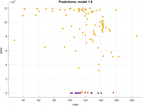
The outputs of the model are shown in Figure 3. Figure 3(a) shows the scatter plot of the training model in which cross(x) symbol shows the misclassified samples. It is plotted between the area and the color value.
Figure 2. Different features of the model
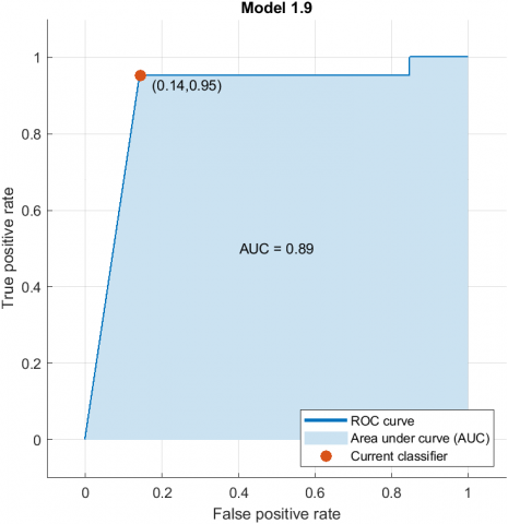
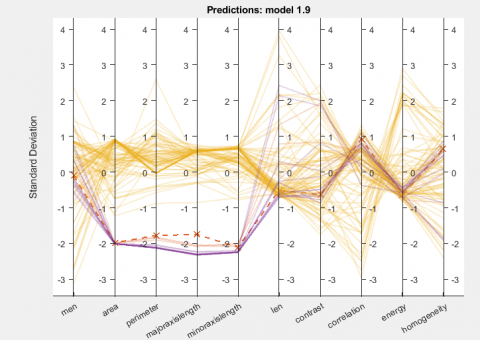
Confusion matrix is an important metric to know about the relevancy of the model. Figure 3(b) shows the confusion matrix which shows the count of correctly classified samples and misclassified samples. These samples belong to five different categories namely severely polluted, moderately polluted, satisfactorily polluted, poorly polluted and very poorly polluted. ROC curve of the model is shown in Figure 3(c). It shows the coordinates of the classification model on the curve. Figure 3(d) shows the parallel plot between the standard deviations and all the features calculated from the image samples.
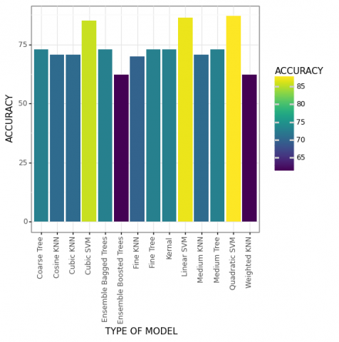
Different classifiers were tested on the dataset to predict the effect of contaminates on the vegetation as shown in Table 3.
From Table 3 best accuracy is highlighted. The plot shows the best accuracy of the different classifiers tested on the dataset as shown in Figure 4.
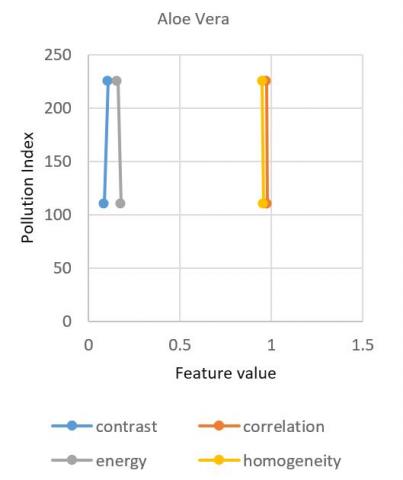
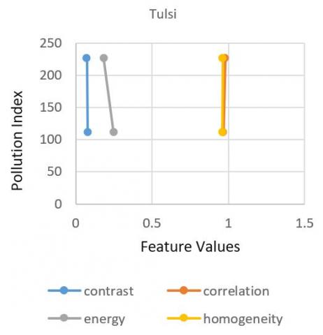
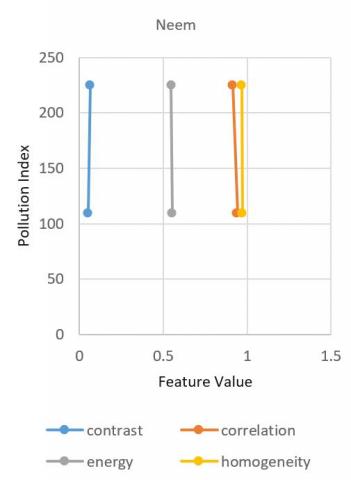
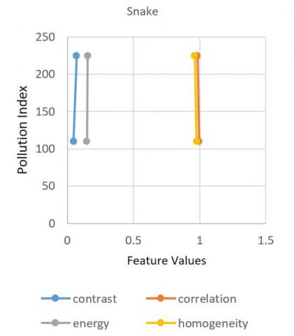
When the pollution index raise from 110(moderately polluted) to 225(poorly polluted) the plant species Aloe Vera’s features like contrast, energy, correlation and homogeneity shows a certain amount of change in its properties as shown in Figure 5. From all the plots there is an observation that When pollution index get increased the contrast in the plant species Aloe Vera, Snake, and Neem gets elevated and other plant species i.e. Spider and Tulsi gets declined. This means intensity of the pixel over its neighboring pixel gets increased in Aloe Vera, Snake, and Neem whereas in Spider and Tulsi shows no effect. In case of energy i.e., the uniform distribution of grey levels gets decreased in Aloe, Tulsi, and Neem and gets increased in Snake and Spider plant. In case of correlation feature, the pixels of the samples got less correlated in all the samples except Tulsi. Homogeneity gets increase in Spider and Tulsi and gets decreased in rest of the samples. On the whole when the pollution index gets more severe, the texture properties of the plant species show a variance. This shows that pollution impacts the plants. So to maintain the oxygen level in the atmosphere, afforestation should be supported more.
3(a)
3(b)
3(c)
3(d)
Figure 3. Results of the prediction model.3(a) Scatter plot to show the correct and incorrect predictions 3(b)Confusion Matrix 3(c) ROC curve 3(d) Parallel Plot for the predictions
Table 3. Accuracies of different models
|
S. NO. |
MODEL |
TYPE OF MODEL |
ACCURACY |
|
1. |
Tree |
Fine Tree |
72.9 |
|
Medium Tree |
72.9 |
||
|
Coarse Tree |
72.9 |
||
|
2. |
Naïve Bayes |
Kernal |
72.9 |
|
3. |
Support Vector Machine |
Linear |
86.4 |
|
Quadratic |
87.1 |
||
|
Cubic |
85.0 |
||
|
4. |
K Nearest neighbor |
Fine KNN |
70.0 |
|
Medium KNN |
70.7 |
||
|
Weighted KNN |
62.1 |
||
|
Cosine KNN |
70.7 |
||
|
Cubic KNN |
70.7 |
||
|
5. |
Ensemble |
Boosted Trees |
62.1 |
|
Bagged Trees |
72.9 |
Figure 4. Accuracies of different classifiers
5(a)
5(b)
5(c)
5(d)
5(e)
Figure 5. Plots for various plant species for the variation of feature values
4.2 Proposed GUI
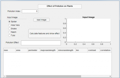
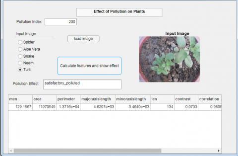
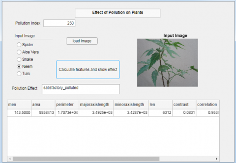
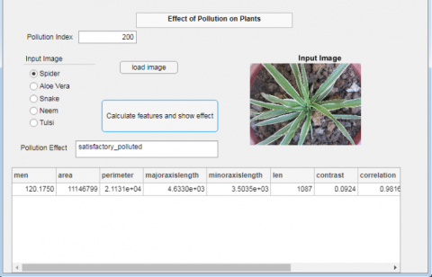
The graphical user interface as shown in Figure 6 has been developed to show the effect of pollution on plants. It has been created by using MATLAB 2020b. First of all, the user is required to enter the pollution index (PI) of the day on which the plant image was captured. Then the name of the plant species is to be selected and the image sample of the plant (Spider, Aloe Vera, Snake, Neem, and Tulsi) will be uploaded. Figure 4 shows the effect of contaminates on different input images as reflected on the GUI. Figure 7(a),7(b), 7(c), 7(d) shows the results for Aloe Vera, Tulsi, Neem, and Spider Plant respectively. The common names of the plant species are also displayed on the screen for easy understanding of the user. All image formats like .jpg, .png,.bmp, .oct are supported for uploading images. When the user clicks on the button ‘calculate features and show effect’, then the pollution effect will be shown in the edit field. Depending upon the evaluation of features (mean, area, perimeter, minoraxislength, majoraxislength, contrast, correlation, energy, homogeineity, and corners length) through the model, it will show the category of pollution effect in which the plant lies. The aim behind the development of this GUI is to provide a user interface for predicting the pollution effect on plants through the proposed model as discussed above.
Figure 6. Graphical User Interface to show the contamination effect
7(a)
7(b)
7(c)
7(d)
Figure 7. GUI with different input images. 7(a) Effect of Contaminates on Aloe Vera. 7(b) Effect of Contaminates on Tulsi. 7(c) Effect of Contaminates on Neem. 7(d) Effect of Contaminates on Spider Plant.
Pollution is one of the most dreadful problems the world is fighting with today. Air pollution being the most devastating of all types, is affecting humans badly and plants are not behind now. Plants too have become a victim and the fact is mostly ignored. It has been proved that pollution has a severe impact on the wellbeing of plants. Oxygen rich and medicinal plants (namely Ocimum Tenuiflorum, Sansevieria Trifasciata, Chlorophytum Comosum, and Azadirachta Indica) were considered for the research and it was found that they have shown a negative response towards pollution. Various features like shape, color, corners and texture have been studied and found to be affected by polluted air. Morphological properties of plants seem to be sensitive and badly impacted by pollution. These properties were successfully used to predict the pollution levels with an accuracy of 85%. The attempt was successful to categorize the plant images into one of the categories on the basis of severity of pollution. The technique of digital image processing was found to be useful in this process and a dataset was created which facilitated in designing and testing of the model using MATLAB 2020b. Finally, a graphical user interface has been designed successfully to facilitate the user for operating on the proposed model. The flora on earth is precious and global attention needs to be drawn towards the issue to save plants by controlling pollution and deforestation.
[1] Central Pollution Control Board (2019). National Air Quality Index. https://www.cpcb.nic.in/National-Air-Quality-Index/?&page_id=National-Air-Quality-Index.Accessed on 10 January 2020.
[2] Valliammal, N., Geethalakshmi, S.N. (2009). Analysis of the classification techniques for plant identification through leaf recognition. Data Mining and Knowledge Engineering, 1(5): 239-243.
[3] Bhatia, M., Mittal, M. (2017). Big data & deep data: minding the challenges. Deep Learning for image processing Applications, 31: 177.
[4] Garcia-Garcia, A., Orts-Escolano, S., Oprea, S., Villena-Martinez, V., Martinez-Gonzalez, P., Garcia-Rodriguez, J. (2018). A survey on deep learning techniques for image and video semantic segmentation. Applied Soft Computing, 70: 41-65. https://doi.org/10.1016/j.asoc.2018.05.018
[5] Anubha Pearline, S., Sathiesh Kumar, V., Harini, S. (2019). A study on plant recognition using conventional image processing and deep learning approaches. Journal of Intelligent & Fuzzy Systems, 36(3): 1997-2004. https://doi.org/10.3233/JIFS-169911
[6] Zhu, Y., Sun, W., Cao, X., Wang, C., Wu, D., Yang, Y., Ye, N. (2019). TA-CNN: Two-way attention models in deep convolutional neural network for plant recognition. Neurocomputing, 365: 191-200. https://doi.org/10.1016/j.neucom.2019.07.016
[7] Linné, C.V. (1788). Systema naturae per regna tria naturae. Humboldt-Universität zu Berlin.
[8] Aggarwal, S., Bhatia, M. (2019). Anatomy of leaf classification techniques. In 2019 International Conference on Machine Learning, Big Data, Cloud and Parallel Computing (COMITCon), pp. 510-513. https://doi.org/10.1109/COMITCon.2019.8862194
[9] Amin, A.H.M., Khan, A.I. (2013). One-shot classification of 2-D leaf shapes using distributed hierarchical graph neuron (DHGN) scheme with k-NN classifier. Procedia Computer Science, 24: 84-96. https://doi.org/10.1016/j.procs.2013.10.030
[10] Bengio, Y., Courville, A., Vincent, P. (2013). Representation learning: A review and new perspectives. IEEE Transactions on Pattern Analysis and Machine Intelligence, 35(8): 1798-1828. https://doi.org/10.1109/TPAMI.2013.50
[11] Singh, K., Gupta, I., Gupta, S. (2010). Svm-bdt pnn and fourier moment technique for classification of leaf shape. International Journal of Signal Processing, Image Processing and Pattern Recognition, 3(4): 67-78.
[12] WHO. Health aspects of air pollution with particulate matter, ozone and nitrogen dioxide.Report 2003 on a WHO working group. Bonn; 2003. http://www.euro.who.int/__data/assets/pdf_file/0005/112199/E79097.pdf.
[13] Stevovi, S. (2010). Environmental impact on morphological and anatomical structure of Tansy. African Journal of Biotechnology, 9(16): 2413-2421.
[14] Haralick, R.M., Shanmugam, K., Dinstein, I.H. (1973). Textural features for image classification. IEEE Transactions on Systems, Man, and Cybernetics, 6: 610-621. http://dx.doi.org/10.1109/TSMC.1973.4309314
[15] Kadir, A., Nugroho, L.E., Susanto, A., Santosa, P.I. (2013). Leaf classification using shape, color, and texture features. arXiv preprint arXiv:1401.4447.
[16] Samuel, N. (1971). Effects of air pollutants on vegetation. In Introduction to the Scientific Study of Atmospheric Pollution, 131-151. https://doi.org/10.1007/978-94-010-3137-0_5
[17] Pourkhabbaz, A., Rastin, N., Olbrich, A., Langenfeld-Heyser, R., Polle, A. (2010). Influence of environmental pollution on leaf properties of urban plane trees, Platanus orientalis L. Bulletin of Environmental Contamination and Toxicology, 85(3): 251-255. http://dx.doi.org/10.1007/s00128-010-0047-4
[18] Giri, S., Shrivastava, D., Deshmukh, K., Dubey, P. (2013). Effect of air pollution on chlorophyll content of leaves. Current Agriculture Research Journal, 1(2): 93-98. http://dx.doi.org/10.12944/CARJ.1.2.04
[19] Aggarwal, S., Bhatia, M., Pandey, H.M. Madaan, R. (2020). Envisaging Variance amid Indian Floras owed to contaminates via SSIM Technique. Indian J. of Env.Protection, In Press.
[20] Aggarwal, S., Bhatia, M., Madaan, R. and Pandey, H.M. (2021). Optimized Sequential model for Plant Recognition in Keras. In IOP Conference Series: Materials Science and Engineering, 1022(1): 012118.
[21] Aggarwal, S., Bhatia, M., Pandey, H.M. (2020). A new method to classify leaves using data visualization: Spreading awareness about global warming. In Proceedings of ICETIT 2019, pp. 1129-1139. http://dx.doi.org/10.1007/978-3-030-30577-2_100
[22] Bhatia, M., Bansal, A., Yadav, D. (2017). A proposed quantitative approach to classify brain MRI. International Journal of System Assurance Engineering and Management, 8(2): 577-584. http://dx.doi.org/10.1007/s13198-016-0465-8
[23] Zhao, A., Tsygankov, D., Qiu, P. (2017). Graph-based extraction of shape features for leaf classification. In 2017 IEEE Global Conference on Signal and Information Processing (GlobalSIP), pp. 663-666. http://dx.doi.org/10.1109/GlobalSIP.2017.8309042
[24] Du, J.X., Wang, X.F., Zhang, G.J. (2007). Leaf shape based plant species recognition. Applied Mathematics and Computation, 185(2): 883-893. http://dx.doi.org/10.1016/j.amc.2006.07.072
[25] Zhang, S., Chau, K.W. (2009). Dimension reduction using semi-supervised locally linear embedding for plant leaf classification. In International Conference on Intelligent Computing, pp. 948-955. http://dx.doi.org/10.1007/978-3-642-04070-2_100
[26] Chaki, J., Parekh, R., Bhattacharya, S. (2018). Plant leaf classification using multiple descriptors: A hierarchical approach. Journal of King Saud University-Computer and Information Sciences. http://dx.doi.org/10.1016/j.jksuci.2018.01.007
[27] Munisami, T., Ramsurn, M., Kishnah, S., Pudaruth, S. (2015). Plant leaf recognition using shape features and colour histogram with K-nearest neighbour classifiers. Procedia Computer Science, 58: 740-747. http://dx.doi.org/10.1016/j.procs.2015.08.095
[28] Rehman, N., Sinha, P. (2013). Colour and texture identification using image segmentation. International Journal on Emerging Technologies, 4(2): 69-75.
[29] Jamil, N., Hussin, N.A.C., Nordin, S., Awang, K. (2015). Automatic plant identification: Is shape the key feature? Procedia Computer Science, 76: 436-442. http://dx.doi.org/10.1016/j.procs.2015.12.287
[30] Murat, M., Chang, S.W., Abu, A., Yap, H.J., Yong, K.T. (2017). Automated classification of tropical shrub species: A hybrid of leaf shape and machine learning approach. PeerJ, 5: e3792. http://dx.doi.org/10.7717/peerj.3792
[31] Palanisamy, T., Sadayan, G., Pathinetampadiyan, N. (2019). Neural network–based leaf classification using machine learning. Concurrency and Computation: Practice and Experience, e5366. http://dx.doi.org/10.1002/cpe.5366
[32] Saleem, G., Akhtar, M., Ahmed, N., Qureshi, W.S. (2019). Automated analysis of visual leaf shape features for plant classification. Computers and Electronics in Agriculture, 157: 270-280. http://dx.doi.org/10.1016/j.compag.2018.12.038
[33] Aggarwal, S., Madaan, R., Bhatia, M. (2020). Morphological based optimized random forest classification for Indian oxygen plants. International Journal on Emerging Technologies, 11(3): 707-714.
[34] Bhatia, M., Bansal, A., Yadav, D., Gupta, P. (2015). Proposed algorithm to blotch grey matter from tumored and non tumored brain MRI images. Indian Journal of science and Technology, 8(17): 1-10. http://dx.doi.org/10.17485/ijst/2015/v8i17/63144
[35] Madaan, A., Bhatia, M., Hooda, M. (2018). Implementation of image compression and cryptography on fractal images. In: Kolhe M., Trivedi M., Tiwari S., Singh V. (eds) Advances in Data and Information Sciences. Lecture Notes in Networks and Systems, vol 38. Springer, Singapore. http://dx.doi.org/10.1007/978-981-10-8360-0_5
[36] Pandey, M., Bhatia, M., Bansal, A. (2016). An anatomization of noise removal techniques on medical images. In 2016 International Conference on Innovation and Challenges in Cyber Security (ICICCS-INBUSH), pp. 224-229. http://dx.doi.org/10.1109/ICICCS.2016.7542308
[37] Pandey, M., Bhatia, M., Bansal, A. (2016). IRIS based human identification: analogizing and exploiting PSNR and MSE techniques using MATLAB. In 2016 International Conference on Innovation and Challenges in Cyber Security (ICICCS-INBUSH), pp. 231-235. http://dx.doi.org/10.1109/ICICCS.2016.7542309
[38] Rother, C., Kolmogorov, V., Blake, A. (2004). “GrabCut" interactive foreground extraction using iterated graph cuts. ACM Transactions on Graphics (TOG), 23(3): 309-314.
[39] Harris, C.G., Stephens, M. (1988). A combined corner and edge detector. In Alvey Vision Conference, 15(5): 5210-5244. http://dx.doi.org/10.5244/C.2.23