Roshan M. Bodile* | Venkata K.H.R. Talari
© 2021 IIETA. This article is published by IIETA and is licensed under the CC BY 4.0 license (http://creativecommons.org/licenses/by/4.0/).
OPEN ACCESS
Electrocardiogram (ECG) is a primary signal utilized in the medical field for the identification and interpretation of pathological and physiological phenomenon. In different real conditions, the ECG is corrupted by many artifacts out of them is power-line interference (PLI). The PLI sternly limits the effectiveness of ECG recordings, and therefore, it is vital to remove PLI for better clinical judgment. In this paper, we have compared discrete wavelet transform (DWT), empirical mode decomposition (EMD), Kalman filter (KF), and KF smoother (KFS) for the elimination of PLI from ECG. These methodologies have experimented on different ECG recordings taken from the MIT-BIH arrhythmia database in the input signal to noise ratio (SNR) range of -10 to 10dB. The simulation results calculated using reconstructed ECG, magnitude spectrum, output SNR, and computational cost indicate that the KFS framework gives better denoising performance compared to KF, DWT, and EMD.
electrocardiogram, discrete wavelet transform, power-line interference, empirical mode decomposition, Kalman filter framework
The cardiac signal is an electrical expression of the contractile activity of the Heart. The electrocardiogram (ECG) is replicating the ionic current flow, those origins the cardiac muscle to contract & relax; consequently, the generation of the understandable graphical time-varying signal. ECG is achieved by recording the potential changes between two electrodes placed on the skin's surface. It is a crucial physiological signal for analysis, judgment, and treatment of severe cardiac diseases. During acquisition, these signals are contaminated or obscured by noises/artifacts such as baseline wander (BW), motion artifacts, electrode movement, and power-line interference (PLI). Furthermore, the use of telemedical applications requires storage and transmission of ECG; artifacts also appear in these applications owing to lousy channel conditions. Removal of such noises, which cause difficulty in diagnosing cardiovascular diseases, is essential for clinical purposes.
Many researchers have contributed to enhancing the quality of the ECG by reducing the noise. The wavelet transform [1-4] is an efficient tool for reducing noise from a non-stationary signal with a low signal-to-noise ratio. The method uses thresholding in the wavelet domain to remove or smooth coefficients of the decomposed signals. The thresholding used in the filtering process is given by Donoho [5, 6], and this method is suited not only to one dimension but also to outstanding works for a two-dimensional signal. Techniques that use shrinkage of coefficients (wavelets) are common for the evaluation of physiological signals. Most ECG wavelet filtering techniques are built on Donoho’s universal theory [4, 7-9]. Sayadi and Shamsollahi [1] introduced a method to reduce noise from noisy ECG recordings using bionic wavelet transform. Singh and Tiwari [10] provided a selection process of mother wavelet applied to remove noise in the wavelet domain. However, the DWT method is sufficiently degraded its denoising performance in low SNR (<=0 dB) conditions. The EMD is another decomposition technique that breaks the signal into different intrinsic mode functions (IMFs) and behaves as a wavelet-like dyadic filter bank [11]. The EMD emerge as a helpful denoising tool [12] for both low and high-frequency noise removal condition. However, the EMD based approach can distort the ECG morphology due to the mode-mixing problem. In the KF framework, tracking PLI and its cancellation using extended KF [13, 14] is studied. In this approach, PLI monitoring and deviations are investigated, which are vital problems in electrical systems. The variation of amplitude and frequency in electrical systems is less, and the use of adaptive filters does not require information about them. In KF [15], and KFS [16] methods, no assumptions are considered regarding the dynamics of the ECG corrupted by PLI. The KFS is an extension of the KF, but it requires a backward and forward filter. The use of this strategy adds better estimation of the PLI besides slight delay in PLI estimation [16]. This study concentrates on one PLI not reviewed any of its harmonics, but it can be extended by adding the dynamics of PLI harmonics.
In this paper, a comparative study of four different methods for eliminating PLI from noisy ECG is presented. Out of them, two are decompositional techniques (DWT and EMD), and others are based on the Kalman filter framework (KF and KFS). This study is considered various aspects performed during experiments such as low to high input SNR (-10 to 10 dB), time-domain analysis for checking reconstructed ECG signal morphology after filtering, quantitative evaluation, and magnitude spectrum to confirm whether PLI is removed or not. Moreover, the study measures the computation cost of all four methods, which may be helpful in real-time application. This study also helpful for selecting denoising methods in a highly noisy environment where PLI sufficiently distorts the ECG morphology.
The outline of the paper is as follows. In Section 2, four denoising methodologies DWT, EMD, KF, and smoother, are presented. The simulation results of four methods are provided using quantitative analysis, filtered signal, and computational time in Section 3. Section 4 gives a discussion about results and the concluding remark given in the last section.
This section has outlined the requirements and necessary implementation details of the DWT, EMD, and Kalman filter framework (KF and KFS).
2.1 Discrete wavelet transform
2.1.1 Wavelet filtering principle
The wavelet transform is a time-frequency method, and it can be term data by using the similarity function correlation with translation and dilation of a mother wavelet [17]. The wavelet transform can be either a continuous or discrete version and represents a signal or data as the addition of wavelets with different scales and locations [18]. In this work, Donoho’s technique is applied to DWT, and the DWT definition is given in Eq. (1) as follows [10, 19]:
$W(d, t)=\sum_{m \in Z} s(m) h_{i, j}(m)$ (1)
where, $W(d, t)$ is dyadic wavelet coefficients, $d=2^{-i}, t=$ $j 2^{-i}, i \in M, j \in Z, d$ is scale(dilation), $t$ is the translation, $s(m)$ is input signal, and $h_{i, j}(m)=2^{i / 2} g\left(2^{i} m-j\right)$ is discrete wavelet. DWT uses a dyadic filter bank to develop the multi-resolution analysis, and it has two filters, namely, high pass filter (HPF) and low pass filter (LPF). The cut-off frequency of HPF and LPF is half the bandwidth of the given signal.
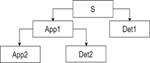
Figure 1. Decomposition of the noisy ECG signal
Wavelet analysis is a combination of the down-sampling and filtering, and it down-samples the given ECG signal by 2. When the ECG signal is passed through LPF, HPF, and down-sampled, the outcome of the process is named as the first level, and decomposition of the signal is given in Figure 1. Here, the noisy ECG (s) breaks into two levels. In the first level, App1 is an approximated coefficient with a frequency range of 0-90 Hz, and Det1 is a detail coefficient with a frequency range of 90-180 Hz. The second level is formed by decomposing App1 into an approximated coefficient (App2:0-45Hz) and detail coefficient (Det2:45-90Hz). The reconstruction process also uses two filters, but down-sampling is replaced by up-sampling with zero padding. Different levels and their corresponding detail frequency are given in Table 1.
Table 1. Detail coefficients at a different level and their corresponding frequency range (Hz)
|
Decomposition level |
Frequency range |
|
Det1 |
90-180 |
|
Det2 |
45-90 |
2.1.2 Thresholding methods
Hard thresholding in Eq. (2) and Soft thresholding in Eq. (3) are widely used algorithms first introduced by Donoho and Johnstone for wavelet-based filtering. The thresholding process is applied to the detail coefficients and is given by
Hard thresholding:
$\hat{D} e t_{i}= \begin{cases}\operatorname{Det}_{i}, & \left|\operatorname{Det}_{i}\right| \geq t h r \\ 0, & \left|\operatorname{Det}_{i}\right| \leq t h r\end{cases}$. (2)
Soft thresholding:
$\hat{D}e{{t}_{i}}=\left\{ \begin{array}{*{35}{l}} \operatorname{sign}\left( {{\operatorname{Det}}_{i}} \right)\left( \left| {{\operatorname{Det}}_{i}} \right|-thr \right), & \left| {{\operatorname{Det}}_{i}} \right|\ge thr \\ 0, & \left| {{\operatorname{Det}}_{i}} \right|\le thr. \\\end{array} \right.$ (3)
where, $\widehat{D} e t_{i}$ are coefficients after thresholding and Deti are coefficients before thresholding.
2.1.3 Denoising parameters and framework
The denoising process involves choosing the five parameters, namely, mother wavelet, type of thresholding, thresholding selection rule, number of levels (decomposition), and rescaling option [19]. In this method, the first stage involves selecting the suitable mother wavelet and its subtype for signal decomposition. The wavelet (biorthogonal and orthogonal) has a different type, and also each wavelet has different subtypes. The mother wavelet considered in this study is Coiflet (coif4) due to its similarity with the ECG morphology. The choice of the level is based on the type of data and experience, and mainly, it is selected based on noise characteristics present at a signal. Here, the PLI frequency is 50 Hz, and hence only two decomposition levels are required. Thresholding has two types, soft and hard, and four types of thresholding rule. The soft thresholding has been used for denoising and the selection of rescaling techniques is available as no scaling, first-level estimation, and level-dependent assessment. The parameters are given in Table 2. The PLI frequency and sampling frequency are known, as shown in Figure 1 and Table 1, two decomposition levels are sufficient for denoising PLI.
Table 2. Wavelet denoising parameters and their range
|
Parameters |
Range |
|
Mother wavelet |
Biorthogonal, Symlet, Daubechies and Coiflet. |
|
Decomposition level |
1-2. |
|
Rescaling approach |
No scaling, single level, and multiple levels. |
|
Thresholding |
Soft or Hard. |
|
Thresholding selection rule |
Rigsure, Minimax, Sqtwolog, and Heursure. |
2.2 Empirical mode decomposition
In conventional EMD, the signal is broken into its subcomponents, called IMFs. If the ECG signal is contaminated by PLI and termed as noisy ECG s(m), then the upper (u(m)) and lower (l(m)) envelopes are measured by interpolating the local minima and maxima with splines. To obtain $\tilde{s}(m)$, the average of envelopes is deducted from s(m), and the signal is produced as:
$\tilde{s}(m)=s(m)-1 / 2\{l(m)+u(m)\}$ (4)
The above process is repeated on $\tilde{s}(m)$ using Eq. (4) and succeeding data until the average value of envelopes is nearly zero. The obtained resulting signal is termed as the first IMF, and for the subsequent IMF that is for the second IMF, the above process is performed on residue r1(m)=s(m)-IMF1(m). Every repetition of the IMF production process generates new IMF and its residue until the process is terminated when residue becomes monotonic. The final signal is represented in Eq. (5) as:
$s(m)=\sum_{j=1}^{I} I M F_{j}(m)+r_{I}(m)$ (5)
where, rI(m) is the residue after the abstraction of IMFI. The decomposition of noisy ECG using EMD is shown in Figure 2. The noisy ECG signal is divided into several IMFs, and the lower IMFs (e.g., IMF1, IMF2, etc.) have high frequency, and the higher IMFs have a lower frequency (e.g., IMF7, IMF8, etc.). The PLI frequency considered in this work is 50 Hz. Most of the ECG features are below this frequency range, and hence to remove the PLI, the first IMF is subtracted from noisy ECG.
Figure 2. Decomposition of noisy ECG into different IMFs
2.3 Kalman filter framework
In this approach, as we consider PLI as interference in ECG, the dynamical model should be formed using the PLI signal. Let us consider, f0 is the PLI and fs sampling frequency, then single tone PLI with an amplitude and phase [15] is expressed as:
$x_{n}=C \cos \left(2 \pi n f_{0} / f_{s}+\phi\right)$ (6)
After applying trigonometric identities and the addition of model error parameter (vn), now the Eq. (6) can be shown in terms of the dynamical model [15] as:
$x_{n-1}+x_{n+1}=2 \cos \left(2 \pi f_{0} / f_{s}\right) x_{n}+v_{n}$ (7)
In practical cases, the model error parameters such as frequency and phase are not additive, as the PLI signal does not have rapid variations. However, to make the above model more flexible, it is common to add (vn) in the Kalman filter approach.
The ECG signal with PLI contamination plus noises or other biosignal is given as
$y_{n}=x_{n}+g_{n}$ (8)
where, xn and gn are the PLI and zero mean random terms, respectively, representing total noises and signals other than PLI. However, this study only considering PLI; we neglecting that gn can be a combination of noises and biosignals.
The dynamical model in Eq. (7) and Eq. (8) is needed to change into state-space form to apply the Kalman filter framework to estimate and eliminate PLI. The state-space form is expressed as:
$\left\{\begin{array}{l}x_{n+1}=B x_{n}+c v_{n} \\ y_{n}=l^{T} x_{n}+g_{n}\end{array}\right.$ (9)
where, $B=\left[\begin{array}{ll}2 \cos \left(2 \pi f_{0} / f_{s}\right) & -1 \\ 1 & 0\end{array}\right], x_{n}=\left[\begin{array}{l}x_{n} \\ x_{n-1}\end{array}\right], c=\left[\begin{array}{l}1 \\ 0\end{array}\right]$, and $l=\left[\begin{array}{l}1 \\ 0\end{array}\right] .$
The above dynamical model in Eq. (9) is ready to apply on PLI contaminated ECG using KF [15] in equations Eqns. (10)-(12) as:
Time Propagation:
$\hat{x}_{n+1}^{-}=B \hat{x}_{n}^{+}$
$P_{n+1}^{-}=B P_{n}^{+} B^{T}+q_{n} c c^{T}$ (10)
Kalman Gain:
$L_{n}=\frac{P_{n}^{-} l}{l^{T} P_{n}^{-} l+k_{n}}$ (11)
Measurement Propagation:
$\hat{x}_{n}^{+}=\hat{x}_{n}^{-}+L_{n}\left[y_{n}-l^{T} \hat{x}_{n}^{-}\right]$
$P_{n}^{+}=P_{n}^{-}-L_{n} l^{T} P_{n}^{-}$ (12)
where, $\quad q_{n}=E\left\{v_{n}^{2}\right\} \quad, \quad k_{n}=E\left\{g_{n}^{2}\right\} \quad, \quad$ priori $\quad \hat{x}_{n}^{-}=$$\hat{E}\left\{x_{n} \mid y_{n-1}, y_{n-2}, \ldots, y_{1}\right\} \quad$ and posterior $\quad \hat{x}_{n}^{+}=$$\widehat{E}\left\{x_{n} \mid y_{n}, y_{n-1}, \ldots, y_{1}\right\}$ estimation of state vector $x_{n}$ with observations $y_{1}$ to $y_{n-1}$. Similarly, the covariance matrices prior $P_{n}^{-}$ and posterior $P_{n}^{+}$ estimates of state vector for the $n^{\text {th }}$ stage are defined, and Kalman gain is $L_{n}$.
The KFS uses the information of future observations to provide better estimates of the present state. This noncausal behavior is expected to give better performance compare to KF [15]. The KFS generally consists of a KF forward step followed by a backward recursion smoothing action. There are two smoothing algorithms, namely, fixed interval or lag smoothing [16]; the fixed lag algorithm is generally used in real applications.
This section is divided into three parts. The first part of the section provides details about datasets and quantitative measures taken during experiments. In the next part, the denoising results obtained after filtering are compared. Finally, the computational cost required for these methods is provided.
3.1 Database and quantitative evaluation
The ECG recordings were taken from the MIT-BIH arrhythmia database [20] for both filtering and analyzing purposes. In this simulation, three ECG signals were taken with record numbers-105, 119 and 210, respectively, in which synthetic PLI (50 Hz) was added to make contaminated ECGs. The ECG records sampling frequency is 360Hz, and for all experiments, 3600 samples or 10 seconds window is used. The ECG with PLI signal s(m)=d(m)+b(m) is filtered, and the reconstructed signal is $\hat{d}(m)$. The signal d(m)is pure and b(m) is PLI; the combination of both is a contaminated signal s(m). The quantitative valuation is measured by using the output signal to noise ratio (SNR) [12]:
OutputSNR$=\frac{\sum_{m-1}^{M} \quad d^{2}(m)}{\sum_{m=1}^{M}\quad\{d(m)-\hat{d}(m)\}^{2}}$ , (13)
and input SNR is given as:
InputSNR$=\frac{\sum_{m=1}^{M} \quad d^{2}(m)}{\sum_{m=1}^{M} \quad b^{2}(m)}$. (14)
3.2 Denoising results
In this subsection, the efficacy of the four methods is evaluated by studying synthetic PLI that appears in the ECG signal. And the synthetic PLI is generated by using sinusoids. All ECG signals considered in this simulation have a sampling frequency of 360 Hz. After the generation of synthetic PLI, this PLI added to pure ECG to obtain a contaminated version of ECG. In DWT, we considered the coif4 mother wavelet with a soft thresholding technique to remove PLI from ECG. As the sampling of ECG is 360Hz, after decomposition of noisy ECG, the PLI appears in second level decomposition for all ECG data. In EMD, the high-frequency noise is available at lower IMFs, and PLI is seen in the first IMF. Therefore, to eliminate PLI from noisy ECG recordings, we just need to subtract the first IMF from noisy ECG. In KF and KFS, all the initial parameters are taken from the researches [15, 16] for filtering purposes.
The clean ECG record “105” and corrupted version of it with synthetic PLI are shown in Figures 3a and 3b, respectively. After applying DWT, EMD, KF, and KFS, the filtering results are shown in Figures 3c-3f. From Figures 3c-3f, it is clear that KFS is more close to the actual morphology of clean ECG, followed by KF, EMD, and DWT. After an inspection of time-domain filtering results, the spectra of the same are shown in Figure 4. The magnitude spectrum also offers the same results given in the time domain. In Figure 4c, the DWT shows some PLI remains in ECG even after filtering the noisy records. The EMD method though it is more suitable for high-frequency elimination, due to the mode mixing problem, some of the content of clean ECG leaks into other IMFs, which causes a decrease in performance. In the case of KF and KFS, as it does not requires any tuning parameters, and it is a stable filter, the denoising performance of the KF framework is high in low as well as high noisy environments.
The filtering results in the time and frequency domain show that the KF and KFS provide better reconstructed ECG after denoising. Now, quantitative analysis is tabulated in Table 3, the DWT gives output SNR of 6.27 to 23.20dB, the EMD offers 19.89 to 22.94dB, the KF provides 21.54 to 22.92dB, and the KFS presents 21.82.23.39dB for input range -10 to 10dB. It is clear from Table 3 that the Kalman framework (KF and KFS) is more suitable for removing PLI from ECGs.
Figure 3. Denoising results for record 105 at 0dB, (a) Noisy ECG, (b) Clean ECG, (c) DWT, (d)EMD, (e) KF, and (f) KFS
Figure 4. Magnitude spectrum, (a) Noisy ECG, (b) Clean ECG, (c) DWT, (d)EMD, (e) KF, and (f) KFS
Table 3. Output SNR for different filtering methods
|
Output SNR |
|
|
|
|
|
Input SNR |
105 |
119 |
210 |
Average |
|
|
DWT |
|
|
|
|
-10 |
6.71 |
6.42 |
5.69 |
6.27 |
|
-5 |
10.92 |
10.68 |
9.86 |
10.49 |
|
0 |
14.46 |
15.39 |
14.69 |
14.85 |
|
5 |
20.13 |
20.22 |
19.52 |
19.96 |
|
10 |
22.38 |
24.92 |
22.31 |
23.20 |
|
|
EMD |
|
|
|
|
-10 |
20.14 |
19.36 |
20.16 |
19.89 |
|
-5 |
21.11 |
20.15 |
21.59 |
20.95 |
|
0 |
22.24 |
21.69 |
21.95 |
21.96 |
|
5 |
23.05 |
23.87 |
22.67 |
23.20 |
|
10 |
22.59 |
24.19 |
22.03 |
22.94 |
|
|
KF |
|
|
|
|
-10 |
22.24 |
21.14 |
21.25 |
21.54 |
|
-5 |
22.56 |
21.56 |
22.55 |
22.22 |
|
0 |
23.33 |
21.84 |
22.73 |
22.63 |
|
5 |
23.69 |
22.32 |
23.21 |
23.07 |
|
10 |
23.11 |
23.01 |
22.64 |
22.92 |
|
|
KFS |
|
|
|
|
-10 |
22.31 |
21.17 |
21.97 |
21.82 |
|
-5 |
22.76 |
21.88 |
22.87 |
22.50 |
|
0 |
23.54 |
22.07 |
23.08 |
22.90 |
|
5 |
24.01 |
22.66 |
23.68 |
23.45 |
|
10 |
23.85 |
23.27 |
23.04 |
23.39 |
3.3 Computational cost
After comparing results quantitatively using output SNR, the reconstructed ECG after removing PLI in time-domain, and frequency domain evaluation using the magnitude spectrum, now methods are compared using the average time taken to remove PLI in the range -10 to 10 dB. In Table 4, the average time to remove 50Hz noise from ECG signals using DWT, EMD, KF, and KFS are shown. From Table 4, we can see that KF and KFS methods require less time, followed by DWT and EMD, respectively.
Table 4. The average computational cost for different denoising techniques
|
Methods |
Computational cost (Seconds) |
|
DWT |
1.4744 |
|
EMD |
2.1956 |
|
KF |
1.0240 |
|
KFS |
1.0244 |
The results section provides valid reasons to eliminate PLI noise from pure ECGs, as the information present in this signal is medically more valuable. The four methods are tested on highly noisy PLI (-10dB) and low noisy (10dB) environments. The DWT and EMD are decomposition-based techniques that divide the given signal into several small parts. The DWT scheme operation depends on the sampling frequency of the given signal, while the EMD is a purely data-based method. It is observed that for input SNR -10 to 0dB, the DWT performance is not good, and also it contains traces of PLI, which means the process is not entirely able to eliminate PLI from corrupted ECGs. After 0dB input SNR, the performance is sufficiently increased and competitive to other methods. In EMD, the denoising performance is nearly constant in the low to high SNR, and the reconstructed ECGs after filtering PLI show that it is a powerful tool for noise elimination.
The KF and KFS methods are used to estimate or track the PLI noise, and filtered signals can be obtained by subtracting this estimate from noisy ECG. The Kalman filter framework is more stable, and its estimates track PLI more efficiently even though in high noise contamination. These techniques convergence depends on the observation noises and covariances of the given model (other words, it merely depends on the ratio of it). The denoising results also provide evidence that the property (optimality) of the KF framework is achieved.
The methods presented in this work are sufficiently general to be applied to other biosignals such as electroencephalogram, electromyogram, etc. These methods are more flexible and can be adapted to PLI harmonics.
Electrocardiogram (ECG) is a primary signal utilized in the medical field for the identification and interpretation of pathological and physiological phenomenon. In different real conditions, the ECG is corrupted by many artifacts out of them is power-line interference (PLI). The PLI sternly limits the effectiveness of ECG recordings, and therefore, it is vital to remove PLI for better clinical judgment. In this paper, a comparative study of four different ECG filtering techniques based on DWT, EMD, KF, and KFS framework is performed. This comparison provides the selection of the best denoising method in a boisterous environment and computational cost. The filtering results show that KF and its smoother methods give the best performance in terms of the ECG morphology, computational cost, and denoising PLI, followed by EMD and DWT.
The study presented here is based on 50Hz PLI. In future work, the experiments will be performed on 60Hz PLI, and also, we have not considered any harmonics of 50 or 60Hz PLI. Therefore, the effect of harmonics in ECG is an area of further scope. The techniques presented in this work are employed on ECG signal only, as these methods are sufficiently general can be applied to other biosignals.
[1] Sayadi, O., Shamsollahi, M.B. (2006). ECG denoising with adaptive bionic wavelet transform. In 2006 International Conference of the IEEE Engineering in Medicine and Biology Society, New York, NY, USA, pp. 6597-6600. https://doi.org/10.1109/IEMBS.2006.260897
[2] Manikandan, M.S., Dandapat, S. (2007). Wavelet energy based diagnostic distortion measure for ECG. Biomedical Signal Processing and Control, 2(2): 80-96. https://doi.org/10.1016/j.bspc.2007.05.001
[3] Holan, S.H., Viator, J.A. (2008). Automated wavelet denoising of photoacoustic signals for circulating melanoma cell detection and burn image reconstruction. Physics in Medicine & Biology, 53(12): 227-236. https://doi.org/10.1088/0031-9155/53/12/N01
[4] Prasad, V.V.K.D.V., Siddaiah, P., Rao, B.P. (2008). A new wavelet based method for denoising of biological signals. International Journal of Computer Science and Network Security, 8(1): 238-244.
[5] Donoho, D.L. (1995). De-noising by soft-thresholding. IEEE Transactions on İnformation Theory, 41(3): 613-627. https://doi.org/10.1109/18.382009
[6] Donoho, D.L., Johnstone, I.M. (1994). Ideal spatial adaptation via wavelet shrinkage. Biometrica, 81: 425-455.
[7] Poornachandra, S. (2008). Wavelet-based denoising using subband dependent threshold for ECG signals. Digital Signal Processing, 18(1): 49-55. https://doi.org/10.1016/j.dsp.2007.09.006
[8] Poornachandra, S., Kumaravel, N. (2005). Hyper-trim shrinkage for denoising of ECG signal. Digital Signal Processing, 15(3): 317-327. https://doi.org/10.1016/j.dsp.2004.12.005
[9] Alfaouri, M., Daqrouq, K. (2008). ECG signal denoising by wavelet transform thresholding. American Journal of Applied Sciences, 5(3): 276-281. http://dx.doi.org/10.3844/ajassp.2008.276.281
[10] Singh, B.N., Tiwari, A.K. (2006). Optimal selection of wavelet basis function applied to ECG signal denoising. Digital Signal Processing, 16(3): 275-287. https://doi.org/10.1016/j.dsp.2005.12.003
[11] Velasco, M.B, Weng B., Barner, K.E. (2008). ECG signal denoising and baseline wander correction based on the empirical mode decomposition. Computers in Biology and Medicine, 38(1): 1-13. https://doi.org/10.1016/j.compbiomed.2007.06.003
[12] Kærgaard, K., Jensen, S.H., Puthusserypady, S. (2016). A comprehensive performance analysis of EEMD-BLMS and DWT-NN hybrid algorithms for ECG denoising. Biomedical Signal Processing and Control, 25: 178-187. https://doi.org/10.1016/j.bspc.2015.11.012
[13] Dash, P., Jena, R., Panda, G., Routray, A. ( 2000). An extended complex kalman filter for frequency measurement of distorted signals. IEEE Transactions on Instrumentation and Measurement, 49(4): 746-753. https://doi.org/10.1109/19.863918
[14] Routray, A., Pradhan, A., Rao, K. (2002). A novel kalman filter for frequency estimation of distorted signals in power systems. IEEE Transactions on Instrumentation and Measurement, 51(3): 469-479. https://doi.org/10.1109/TIM.2002.1017717
[15] Sameni, R. (2012). A linear kalman notch filter for power-line ınterference cancellation. In: The 16th CSI International Symposium on Artificial Intelligence and Signal Processing, Shiraz, Iran, pp. 604-610. https://doi.org/10.1109/AISP.2012.6313817
[16] Warmerdam, G.J.J., Vullings, R., Schmitt, L., Van Laar, J.O.E.H., Bergmans, J.W.M. (2016). A fixed-lag Kalman smoother to filter power line interference in electrocardiogram recordings. IEEE Transactions on Biomedical Engineering, 64(8): 1852-1861. https://doi.org/10.1109/TBME.2016.2626519
[17] Novak, D., Frau, D. C., Eck, V., Pérez-Cortés, J.C., AndreuGarcía, G. (2000). Denoising electrocardiogram signal using adaptive wavelets. In: BIOSIGNAL 2000, Brno, Czech, pp. 18-20.
[18] Zhang, Y., Wang, L., Gao, Y., Chen, J., Shi, X. (2007). Noise reduction in Doppler ultrasound signals using an adaptive decomposition algorithm. Medical Engineering & Physics, 29(6): 699-707. https://doi.org/10.1016/j.medengphy.2006.08.002
[19] El-Dahshan, E.S.A. (2011). Genetic algorithm and wavelet hybrid scheme for ECG signal denoising. Telecommunication Systems, 46(3): 209-215. https://doi.org/10.1007/s11235-010-9286-2
[20] Goldberger, A.L., Amaral, L.A.N., Glass, L., Hausdorff, J.M., Ivanov, P.C., Mark, R.G., Mietus, J.E., Moody, G.B., Peng, C.K., Stanley, H.E. (2000). PhysioBank, PhysioToolkit, and PhysioNet: Components of a new research resource for complex physiologic signals. Circulation, 101: 215-220. https://doi.org/10.1161/01.CIR.101.23.e215