Fatma Özcan* | Ahmet Alkan
© 2021 IIETA. This article is published by IIETA and is licensed under the CC BY 4.0 license (http://creativecommons.org/licenses/by/4.0/).
OPEN ACCESS
One of the goals of neural decoding in neuroscience is to create Brain-Computer Interfaces (BCI) that use nerve signals. In this context, we are interested in the activity of nerve cells. It is possible to classify nerve cells as excitatory or inhibitors by evaluating individual extra-cellular measurements taken from the frontal cortex of rats. Classification of neurons with only spike timing values has not been studied before, with deep learning, without knowing all of the wave properties and the intercellular interactions. In this study, inter-spike interval values of individual neuronal spike sequences were converted into recurrence plot images to analyze as point processing, image features were extracted using the pre-trained AlexNet with CNN deep learning method, and frontal cortex nerve cell type classification was made. Kernel classification, SVM, Naive Bayes, Ensemble, decision trees classification methods were used. The accuracy, sensitivity and specificity evaluate the proposed methods. A success of more than 81% has been achieved. Thus, the cell type is defined automatically. It has been observed that the ISI properties of spike trains can carry out information on cell type and thus neural network activity. Under these circumstances, these values are significant and important for neuroscientists.
classification, deep learning, excitator, inhibitor, neuroscience, point processing, recurrence plot, spike, excitatory units
Neuroscience is based on the study of the nervous system. It is an interdisciplinary field in which medicine, biology, psychology, chemistry, mathematics, physics and engineering sciences work together. Central and peripheral nervous system, brain, neuron, electrical potentials, synaptic connections, neural networks, nervous system development, sensory systems, motor control, learning, memory, language, cognition are some of the topics of interest to neuroscientists [1].
When a resting nerve cell is stimulated, a reaction called action potential (spike) occurs. Action potential is a potential change determined by differences in intracellular and extracellular chemical concentrations. The action potential (spike) measured from the nerve cell is a sudden electrical activity, as shown in Figure 1. Depending on the stimulus or situation, the spikes that are emitted into the neuronal cell, are generated or blocked.
Figure 1. The action potential [2]
With external sensory stimuli application such as light, sound, taste, odor and touch, sensory neurons show their activities with spike sequences in different temporal patterns. This sensory stimulus information is encoded and transmitted to the brain and its environment. This is considered the main way of transferring information in the nervous system [2]. Neuroscientists are studying the features of the sequence (time, propagation frequency, spiking rate, peak width, etc.) and the intercellular interactions to understand how the brain behaves (neuronal coding) depending on the stimulus or situation (sleep, wakefulness, hunger, thirst) to be analyzed.
The frontal cortex is a region of the brain responsible for voluntary motor coordination and language. Studies are conducted to find out what type of neuronal activity these functions are involved we want to work with data acquired during one of these studies [3, 4].
In order to understand variable neural network architectures, it is important to know the basics of the methods of recording neural activities. The most invasive measures consist in placing electrodes in the brain and recording signals [5].
Figure 2. The basics of the methods of recording neural activities [6]
Extracellular multineural records are made using multi-electrodes (Figure 2). At each electrode, the electrical activity of one neuron is measured as well as the electrical activity of neighboring neurons [7]. As can be seen in Figure 3A, two types of signals can be distinguished from the obtained measurements: The local field potential (LFP) and the action potential sequence (Figure 3B). Next, by a spike sorting process, a registered spike signal sequence is associated with each cell (Figure 3C) [7-10]. By using the individual neuronal signal and intercellular interactions, cell types are identified as excitatory or inhibitory.
Figure 3. Extracellular multineural records. A: Obtaining spike sequences for all cells, from extracellular recording [10]. B and C: Spike sorting of three nerve cells [8]
Figure 4. Neural decoding: Different neural input data (top) and prediction of many different outputs (bottom) [5]
The raw waveform sequence is reduced to vectors time values. In this process, the presynaptic and postsynaptic interaction information of neurons, spike width and trough-to-peak information are removed. This state of the data shows the spiking rate or time encoding, enabling the examination of the temporal structure in one or more cells.
Spike sequences can help to understand the features of neural coding and decoding. In the coding process, neural activity is the result of a biological signal (stimulus). During decoding, the relationship is reversed and the signal (stimulus) is predicted from neural activity (Figure 4).
One of the goals of neural decoding is to create brain- computer interfaces (BCI) that use nerve signals. This could allow, for example, patients with neurological or motor diseases to control a robotic arm. An additional objective of neural decoding is to better define the relationship between neural activity and the environment. To improve the accuracy of decoding, it is possible to compare work done with different experimental conditions (different brain regions, different cell types, different types of subjects). Neural decoding is used to predict movement, speech, vision, etc. [5]. As shown in Figure 4 [5]. For example, in a decoding process, the spike sequence is sent to the decoder and an attempt is made to obtain the applied stimulus information. While the time coding of the sequence was used in the decoding process in previous works [11], there have not been many studies using deep learning [5].
The coding properties of spikes can convey information about the cell type. The classification of individual neurons informs us about the global state of activity (sleep or wakefulness) of the neural network (neural community) [12].
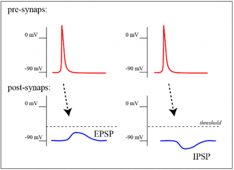
A neurotransmitter affects a neuron in three ways: with excitatory, inhibitory (Figure 5) or regulatory properties. In the excitatory nerve cells, pyramidal cells, the presynaptic neuron supports the generation of the action potential signal in the postsynaptic neuron, while this is blocked in the internal inhibitory nerve cells. Whether a neurotransmitter type depends on the receptor to which it binds [13]. Recognizing the excitatory or inhibitory properties of nerve cells in a particular area of the brain, provides information about the "learning" of the neural network [14]. In the measurements performed, the supposedly stimulating (excitatory-pyramidal cells) or suppressive (inhibitor-interneuron cells) properties of the cells must be highlighted.
Figure 5. Cell type: (left) excitatory or epsp (= excitatory post synaptic potential), (right) inhibitory or ipsp (inhibitory post synaptic potential [15]
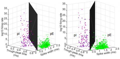
Figure 6. Classification of putative excitatory (pe) and putative inhibitory (pi) cells as a function of trigger frequency, spike width and trough-to-peak time using the raw waveform [3]
By evaluating extracellular signals measured from the frontal cortex of laboratory animals, it is possible to classify nerve cells as either excitatory or inhibitory. This process has already been successfully carried out using the raw waveform or cross-correlogram method that evaluates intercellular interactions (Figure 6). Unfortunately, the latter method requires manual control of the result by the neuroscientist and is a laborious procedure [3].
The trigger rate is higher in inhibitory neurons. This is due to the need for heavier measurement parameters than excitatory neurons. This explains the low amount of inhibitory cell measurement [14].
A fine analysis of the time structure in spike series can be used to find the characteristics of the cells. The classification of excitatory and inhibitory cells with only recorded spike timing sequences, without knowing their wave properties and inter-cellular interactions, has not been previously performed by deep learning. Can we now understand the neuronal activity of the frontal cortex through the temporal coding of spikes? Can we get information to decode this encoding?
In probability theory and statistics, discrete series of events such as spike time sequences are analyzed as point processing. These time series are both dynamic and stochastic. Its properties therefore change over time. This signal is a series of binary values (0-1). Spike series are difficult to analyze and compare because there are few point processing analysis methods.
Recently, many studies have attempted to determine the identity of neurons by evaluating the distance metric in spike timing [16]. One of them is the interval Inter-Spike (ISI) [12, 17]. In neural coding, the distance between two spikes can contain important information [18]. The ISI value has been shown to be effective in classifying cell type in the brain [17]. In spike trains, a recurrence graph was used to visualize the dynamic changes of the ISI measurements. The recurrence graph converts each value into an Inter-Spike interval matrix [12]. This process allows to draw two-dimensional graphs, which allows to study many spike sequence properties such as serial dependence, chaos and synchronization [19]. In our study, the ISI values obtained from spike timing sequences will be converted into recurrence plot images.
Over the past decade, deep learning has become the most successful method in many machine learning studies, from image segmentation to speech recognition. The popularity of deep networks in a variety of other fields has spawned a new generation of applications in neuroscience. Deep learning has proven to be an important tool for increasing the accuracy and flexibility of neural decoding in many areas. Further development of these areas of neuroscience can be expected in the future [5]. Deep learning techniques can also be considered effective with spike sequences converted into images.
Classifying nerve cells as excitatory or inhibitory using extracellular measurements of the frontal cortex of rats, Watson et al. [3] obtained about 90% accuracy in the waveform-based classification. He obtained this result using the raw spike waveform. Classification by the cross-correlogram method, which is not fully automatic, requires intensive manual supervision by the neuroscientist and uses intercellular interactions, was close to 100%. In our study, we will use this output as ground truth in the classification of spike time sequences (without recognizing the intercellular interaction, spike width, trough-to-peak properties of the spike).
In his study entitled "Computational classification approach to profile neuron subtypes from brain activity mapping data", Li et al. [17] classified pyramidal excitatory neurons and interneurons using spike wave, Inter-Spike interval and spiking rate. They developed two pyramidal cell types in the cortical and subcortical regions of awake and in slow wave sleep-SWS animals. This was done using the inter-spike interval. They also identified two types of dopaminergic (DA) neurons in the mesencephale-VTA (ventral tegmental region). In the classification of cell subtypes with the ANOVA and Tukey tests, he obtained high accuracy.
Lazarevich et al. [12] in their paper "Neural activity classification with machine learning models on inter-spike interval series data", obtained 60% success in the classification of excitatory and inhibitory cells with the machine learning method, kNN (k-nearest neighbors). With the manual feature extraction method (tsfresh, Python package), he obtained more than 65% accuracy by using several classification algorithms (random forest, trees, boost). We used the same dataset in our work.
Glaser et al. [20] in his work entitled "machine learning for neural decoding", he tried to study the decoding of spike neural activity with machine learning methods. They used Neural Networks, Boosted trees, Support Vector Machines, on spike sequences from the motor cortex, somatosensory cortex and monkey hippocampus. In this study, to determine the instant movement speed, about 80% accuracy was obtained for the motor cortex, by the Ensemble approach. This success was about 60% in the hippocampus.
In 1995, Şeker et al., and Hinton et al. developed, using the wake-sleep algorithm, a network with hundreds of hidden layers, 6 of which were fully connected. They saw that this was possible, even though the training took two days [21, 22]. Chagas et al, in a study entitled "Functional analysis of ultra high information rates conveyed by rat vibrissal primary afferents", they were able to predict the position, speed and acceleration of the rat whiskers from spike sequences of rapidly adapting and slowly adapting afferent cells with an accuracy of 80-90% [23]. Fang et al. [18] in their study entitled "Spiking neural networks for cortical neuronal spike train decoding", obtained about 82% of accuracy in classification with the SNN approach in motion control encoding. Saif-ur-Rehman et al. [24] with the application of SpikeDeeptector, performed a classification study to distinguish noise and spikes from raw neural signals. They obtained an accuracy of 98.9% using CNN and FNN (Fully connected Neural Networks) deep learning methods [24]. In our study, the importance of temporal structure and spiking rate in cell type classification will be revealed by using only the spike sequence, and not the raw neural signal as in the study of Saif-ur-Rehman et al. [24]. Jouty et al. [25] in his study entitled "Non-Parametric Physiological Classification of retinal ganglion cells in the mouse retina", he achieved great success in classifying 1000 different retinal ganglion cells by comparing two spike sequences. Markanday et al. [26] in his study entitled "Using deep neural networks to detect complex spikes of cerebellar Purkinje cells", succeeded in distinguishing complex and simple spikes from cortex signals with the CNN deep learning network. This study is in the framework of spike sorting. Racz et al. [27] in his study entitled "Spike detection and sorting with deep learning", applied the CNN method to the raw wave from the motor cortex and contributed to brain-computer interface (BCI) studies by predicting the activity of 20 neurons with an accuracy of 89%. Livezey and Glaser [28] in his work entitled "Deep learning approaches for neural decoding: From CNNs to LSTMs and spikes to fMRI", reviewed deep learning approaches for neural decoding. He stated that deep learning has proven to be a useful tool for increasing the success and flexibility of neural decoding in a wide variety of tasks, and that further development of these scientific fields can be expected in the future [5].
Lin et al. [29] in their study entitled "Evaluation of vertical ground reaction forces pattern visualization in neurodegenerative diseases identification using deep learning and recurrence plot image feature extraction", using deep learning, made five classifications of neurodegenerative diseases with recurrence plots and obtained an accuracy of almost 100% [28]. Garcia-Ceja et al., in their study entitled "Classification of Recurrence Plots' Distance Matrices with a Convolutional Neural Network for Activity Recognition", obtained 90.1% accuracy using the convolutional neural network (CNN) with the recurrence plot [30]. Afonso et al. [31], in their study entitled "A recurrence plot-based approach for Parkinson's disease Identification", converted the signals from the sensors, which are on the pen used, to plot a recurrence plot, for Parkinson's disease detection and they improved the accuracy rate in detecting the disease with 87% [32].
The use of recurrence plot and CNN to classify spike sequences was not found in the literature.
Neuroscientists are trying to understand more about how the different areas of the brain are connected to the external world. This might be useful, for example, to control human-computer interface devices by predicting the code for cerebral activity [20, 27]. One of the objectives of neural decoding is to provide, in a sick individual who has had treatment, a result similar to that of a healthy individual. For example, it may be aimed at developing a treatment that provides, in a patient with various complications of neuronal activity during sleep, results obtained from a healthy individual. Neuronal decoding is a classification used to associate nervous signals with certain variables [20]. To date, in deep learning techniques have been very successful in decoding neuronal activity (stimulus prediction from a spike sequence) [33] or in neural coding (prediction of neural activity from a stimulus) [34].
Well, can neural network models in deep learning help us to understand the neural networks of the brain? With these models, can temporal structure be used without all the characteristics of the neural signal? As in the brain, in the execution of the model in question, can we process few data to obtain the information required?
Knowing whether cells are excitatory or inhibitory can help us understand how individual cells interact with each other, and thus learn about the activity of the neural network (neuronal community) in order to understand the neuronal code. Some properties of spike trains may contain information about the cell type [12].
As a hypothesis, a fine analysis of the temporal structure can be considered useful to find the properties of cells with spike trains. This is thought to be decisive in the analysis of an individual neuron. Can we understand the neuronal activity of the frontal cortex with an analysis of the temporal coding of the spike? The spiking rate is higher in inhibitory neurons than in excitatory neurons [14]. In the study, we can see that the temporal structure is distinctive. With just the temporal sequence of the spike, can we still classify the cells as excitatory or inhibitory? What accuracy values can we achieve under such conditions, even if the results of a raw signal are not achieved?
In classification, studies using deep learning approaches on raw neural waveforms, have been very successful. However, in the literature, we have never encountered cell type classification with a temporal spike sequence studied with deep learning methods. During sleep and wakefulness situations, on measurements of the frontal cortex of the brain, statistical and machine learning models have been used to distinguish excitatory and inhibitory neurons. However, these classification studies have not been very successful. It may be possible to facilitate, accelerate and obtain new information with deep learning methods. With this type of data, can we use methods that have not been used before and improve accuracy? Can we use a small amount of data to have a significant result in our deep learning system?
The temporal structure of spikes, the dynamic process of generating action potentials from individual neurons or the distance between spikes may have a significant role in the transfer of information via neurons [18]. The classification of excitatory and inhibitory cells with only temporal sequences and the Inter-Spike interval, without knowing all the features of the raw signals and cellular interactions, has not been previously performed by deep learning. How can we carry out the work in this context? Deep learning techniques are thought to be effective with the conversion of signals into images. The aim of this study is to classify cell types by converting the ISI values of the individual neuronal sequence into a recurrence plot image, extracting the image features with deep learning, as shown in Figure 9. The sleep-wake state is not taken into consideration in this study in which we want to see the applicability of the methods in question.
The computational neuroscience aims at developing mathematical computational models inspired by the neurosciences [35]. With these models, artificial intelligence, machine learning and deep learning solutions used in engineering have been developed. In our work, convolutional neural networks can be used to better understand the brain's nerve cell activity. We will try to see if the inspired model can help to further our understanding of the source of inspiration. In addition, our work may eventually help us to understand the multiple issues involved in the interaction between the neurosciences and computer science.
3.1 Data
In our study, a high-quality dataset with recordings of neural firing activity is used. The open-access fcx-1 dataset, which is freely available from the Collaborative Research in Computational Neuroscience (CRCNS) repository (http://crcns.org/), will be used [36].
In the dataset fcx-1 [3, 4], 11 male Long Evans rats aged 4 to 7 months without any particular behavior, task or stimulus were used. During sleep and wake states, multielectrode arrays installed on a microdrive allow for multineural extracellular recordings by accessing the frontal cortex region. For this purpose, 256-channel Amplipex recording implants were used. Spiking activity and LocalField Potential (LFP) signals are distinguished from recordings. The Local Field Potential (LFP) is derived from the obtained signals using a 20 kHz low-pass filter. LFPs are thought to be the sum of the input activities of local neurons [5]. With the 800 Hz high-pass filter, the action potential signals are separated and thresholded. The spike sorting applications, KlustaKwik and Klusters, allow the identification of the spike train of each individual neuron by the clustering or classification process. In general, cells with a firing rate of < 5 Hz and a width of > 300 µs are excitatory, cells with a firing rate of > 10 Hz and a width of < 250 µs are inhibitory cells [17].
Data from approximately 40 cells were considered for each animal. There were 27 recording sessions containing an average of 2 wake-sleep episodes wherein at least 7 minutes of wake are followed by 20 minutes of sleep. Measurements lasted between about 1 and 8 hours [5, 37, 38]. Sleep states are determined according to the properties of the LFP and EMG signals. Sleep or wakefulness was not addressed in this study. Again, in this study it is assumed that the time and amplitude properties of each action potential do not change. Vectors of spike times was used for each cell.
Approximately 1121 stable units (neurons) were recorded, with 126 putative inhibitory cells and 995 putative excitatory cells. The spike times trains were classified into neuron/experiment/animal.
Several classifications can be solved with this dataset:
- classification of excitatory and inhibitory cells with spike trains with a similar mean neural firing rate,
- classification of the status of sleep and wakefulness activity.
In our study, the first point above will be discussed using the vectors of spike times.
In this study, we want to show that success rate is high with deep learning methods using fewer data, without the necessity of all the data set. The reason why we want to work with less data is that the time saving is important as well in recording signals, in all signal processing steps, in the conversion of the signals into images and in the acceleration of the deep learning process.
3.2 Tools
The study was executed with Matlab2020a. A computer with an Intel CoreTM i5-3210M 2.5 GHz processor, 6 GB RAM and an NVIDIA GeForce GT640M GPU graphics board was used.
3.2.1 Preprocessing
The multitude of features can sometimes interfere with proper operation. Therefore, one of the most common pre-processing techniques is downsizing or feature selection. Feature selection is the process of identifying and removing information that is irrelevant and unnecessary. The selection of features in our study will be done automatically by the convolutional neural network (CNN). By reducing the size of the data, the learning algorithms can work faster and more efficiently.
A classification problem occurred with this dataset. The images of excitatory and inhibitory cells with the same firing rate patterns are similar. In our study, images that are likely to cause misclassification were not removed.
The number of spikes and the recording time in the sequence of each neuron are variable, so the length of the sequence is not the same. One way to normalize the length of the chains is to divide them into equal parts. They can be divided into segments of equal time or segments of equal number of points. In this study, each series will be divided into equal segments of 25 points. In other words, each sequence is divided into windows of 25 ISI and the number of data is therefore increased. We did not choose the number of points less than 25 to have enough information on an image, and not more than 25 to not lose the resolution of the image.
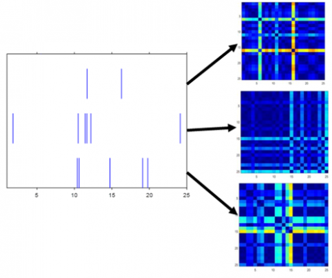
Deep learning techniques would be effective by converting spike trains into images. The spike train that we have, could be plotted as a raster plot. On Figure 7A neuronal spiking activity of an excitatory cell is plotted over a duration of about 6 hours. On Figure 7B neuronal spiking activity of an inhibitory cell is plotted. However, since the temporal properties of the data are more marked, it was preferred to obtain images in the form of a recurrence plot using Inter-Spike interval values. In Figure 8, 8A shows the Recurrence plot of 25 ISI of the excitatory cell recordings. The 8B shows Recurrence plot of the inhibitory cell recordings.
The spike sequences were collected from 6 neurons, 3 excitators and 3 inhibitors from 5 of the 11 animals in the dataset summarized in Table 1. As shown in Figure 10 and Figure 11, we obtained 100 recurrence plot images for each cell. As a result, 1500 recurrence plot images of excitatory cells and 1500 recurrence plot images of inhibitory cells are generated (Figures 11 and 12). The images to be trained with CNN are in RGB 227x227x3 and jpeg format. 70% (2100 images) of the 3000 images are used for training and 30% (900 images) for the test.
Figure 7. 0-22000 seconds of raster plot that we plotted in Matlab: A: Neuronal spiking activity of an excitatory cell (blue). B: Neuronal spiking activity of an inhibitory cells (red)
Figure 8. Recurrence plot. A: Recurrence plot of 25 ISI of the excitatory cell recordings. B: Recurrence plot of the inhibitory cell recordings. (dark blue: close to 0 seconds, burgundy: 30 seconds or more) visualized in Matlab
Table 1. Features of dataset (pe: Putative excitatory, pi: Putative inhibitory) [3]
|
Animal name |
Anatomical Location |
Number of Sessions |
pe Units / Session |
pi Units / Session |
|
BWRat17 |
ACC |
2 |
38.5 |
4 |
|
BWRat18 |
M2 |
1 |
34 |
6 |
|
BWRat19 |
M2 |
2 |
44 |
11.5 |
|
BWRat20 |
ACC |
2 |
38.5 |
5.5 |
|
BWRat21 |
mPFC |
3 |
19.7 |
2 |
|
Dino |
mPFC, ACC |
8 |
41.8 |
3.9 |
|
B22 |
OFC |
3 |
34 |
7.3 |
|
Bogey |
mPFC |
1 |
33 |
3 |
|
Splinter |
OFC |
2 |
33.5 |
5.5 |
|
Rizzo |
OFC |
2 |
57 |
2.5 |
|
Templeton |
OFC |
1 |
10 |
0 |
3.2.2 Feature change: Recurrence plot
According to Eckmann et al. [37] the Recurrence Plot (RP) is a means of visualizing repetitive behaviors in time series. Recently, the recurrence plot, initially proposed as a visual analysis tool, has been used to extract dynamic properties (dynamism, synchronization, regime changes) from time series data of complex systems [38]. The conversion of the original 1D (time domain) signal into a 2D image format shows the temporal structure. The ISI distance matrices composed of our data can be recorded as images [39]. The recurrence plot provides a series of points of size N × N in square shape. N is the number of cases considered (Table 2). The points of the table are placed in the coordinates (i, j) with the value $D_{i, j}$(x) as shown in formula (1) [31].
$D_{i, j}(\mathrm{x})=\left\|\overrightarrow{x_{i}}-\overrightarrow{x_{j}}\right\|$ (1)
$\mathrm{X}=\left\{\overrightarrow{x_{1}}, \overrightarrow{x_{2}}, \ldots, \overrightarrow{x_{n-1}}, \overrightarrow{x_{n}}\right\}$ are ISI values in the matrix. All values are entered symmetrically. If $D_{i, j}$(x) is divided by the largest value of X, the data are normalized and all values are between 0 and 1. On the other hand, neural data are both dynamic and stochastic. Therefore, it was observed that the difference between the normalized excitatory and inhibitory images diminished. We therefore chose not to normalize the values. If the difference between $\overrightarrow{x_{i}}$ and $\overrightarrow{x_{j}}$ is too small, the pixel will be dark, and if it is large, the pixel will be lighter. In addition, with these tools, texture characteristics (texture) can be analyzed on recurrence plot.
Table 2. Recurrence plot matrix of 5 ISI values points
|
|
1 |
2 |
3 |
4 |
5 |
|
1 |
0 |
0.0524 |
0.5194 |
0.0383 |
0.0771 |
|
2 |
0.0524 |
0 |
0.4670 |
0.0140 |
0.0247 |
|
3 |
0.5194 |
0.4670 |
0 |
0.4811 |
0.4423 |
|
4 |
0.0383 |
0.0140 |
0.4811 |
0 |
0.0387 |
|
5 |
0.0771 |
0.0247 |
0.4423 |
0.0387 |
0 |
Figure 9. Flowchart from recording to cell type γ classification
Figure 10. Obtaining recurrence plots from raster plots: bwrat21_121113 first inhibitory cell, 25 ISI, 3 images
Figure 11. Obtaining recurrence plots from raster plots: bwrat21_121113, second excitatory cell, 25 ISI, 3 images
Figure 13. Model construction: architecture of the convolutional neural network (CNN)
3.2.3 Artificial intelligence, deep learning
The fields of neuroscience and artificial intelligence (AI) have a closely related history. A better understanding of biological brains is found to play a key role in building intelligent machines. Neuroscience studies in humans and animals have led to the development of studies in artificial intelligence. Taking this further, intelligent algorithms have the potential to offer new insights into the foundations of intelligence in the human and animal brain. This general narrative curve shows how ideas are exchanged between neuroscience and artificial intelligence [40].
Deep learning is important for people who want to understand how perception and cognition are derived from neural activity. Neural network model systems are based on biological brains and use only biologically reasonable calculations. Advances in deep learning are bringing us closer to understanding the brain via the various fields of neuroscienced [40].
With deep learning techniques that have shown great success in image and natural language processing, much greater success can be achieved in this study. In deep learning, there is a structure based on learning several levels of data characteristics. Deep learning is essentially based on learning data representation [21].
The human brain can learn with much less data than deep learning. Moreover, deep learning uses many more neural layers than the human brain [11]. In the coming years, neural network learning will be possible with more robust and generalized performance by becoming less dependent on large labeled data sets [41]. In this work, we will use a reduced number of data sets for learning.
3.2.4 Convolutional Neural Networks (CNN)
The convolutional neural network (CNN) in fact imitates the human cerebral cortex. The CNN algorithm is inspired by the visual processing center of animals.
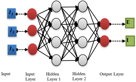
CNN is a Multi Layer Perceptron-MLP. The convolution process is the response of a neuron to stimuli from its own stimulation field. As shown in Figure 14, CNN consists of one or more fully connected layers, like a neural network [21].
Figure 14. Deep neural network with 3 inputs and 2 outputs
The architecture of a CNN is designed to have a 2D input structure (image or signal). One advantage of CNNs is that they are simpler to train. CNNs have far fewer parameters than other fully connected networks [29].
In general, a CNN is composed of convolution, pooling and fully connected layers. The convolution layer consists of a series of filters that apply to the width and height of the input image. At the convolution layer, there is learning of hierarchical patterns, which is not the case for fully connected layers. The surface layers learn small local patterns, while subsequent layers learn more abstract patterns than the previous ones. The pooling layer divides the input image into non-overlapping rectangular subregions to which a function is applied. Pooling layers reduce the size of the data from the convolution layer, which reduces the number of parameters and makes the process of learning more computationally efficient [30, 39]. In image recognition tasks, feature detection is very important rather than the exact location of that feature. This is achieved at the level of the pooling layer which provides translation invariance. As a result, at the expense of spatial resolution, less significant data is eliminated and the detected features are preserved in a minimal representation.
Max pooling and average pooling are the most commonly used reduction methods. Max pooling has shown more rapid convergence with improved performance [42]. Thus, current work tends towards max pooling. Max pooling is used in the Alexnet architecture.
The overlapping window method at the pooling layers can reduce the risk of overfitting. This reduction can limit the depth of a network and ultimately its performance. This problem has prompted researchers to find alternative methods to improve or replace the pooling layer. One approach is to use "fractional filters instead of common filters" [43]. Another option is to remove the pooling layers and perform the reduction by increasing the pitch in the convolutional layers [44]. These solutions remain current research topics, and will not be addressed in our work.
After stacking the convolution and pooling layers, the last layer is usually used to obtain the final classification [29].
3.2.5 Transfer learning
With the knowledge acquired, human beings have an excellent ability to generalize or transfer learning to areas not previously seen. For example, a person who can drive a car can act when confronted with a vehicle that has never been used before. On this basis, artificial intelligence architectures that can show strong generalization or transference have been developed. In the neuroscience literature, one of the distinctive characteristics of transfer learning has been the ability to reason. AI researchers have made progress in building deep networks that meet these expectations [40]. With transfer learning, there can be rapid learning and connections can be made with other data [40]. In this study, an AlexNet pretrained model architecture was used because the ratio of processing time to classification accuracy performance is judicious [45].
A pre-trained AlexNet CNN is used with the MATLAB R2020a Deep Learning ToolboxTM [45]. Kirzhevsky et al. trained a deeply convolved neural network, called AlexNet. The latter, contains 1.2 million high resolution images from 1000 different labels. The architecture consists of 25 layers, including an input layer, five convolution layers, seven ReLU layers, two cross-channel normalization layers, three 2D max-pooling layers, three fully connected layers, two regularization layers, a softmax layer, and an output layer. The shallow layers, which generally produce fewer features, have higher spatial resolution and a greater number of activations. The deep layers contain higher level features created by features from the surface layers (Figure 13) [29].
In this work, a pre-trained AlexNet [45] was used to obtain a balance point between accuracy performance and computation time. Indeed, with Alexnet, the classification accuracy is much better than classical CNNs such as LeNet. Moreover, AlexNet consumes less time compared to advanced CNNs such as GoogLeNet or ResNet) [29].
3.2.6 Image classification
The purpose of image classification is to classify images into several classes, according to a labeling. We can list the steps of the operation as follows:
- Input: consists of N images, each labeled by one of the K different classes. These data are called training sets.
- Training: learns what the classes look like using the features of the input data.
- Evaluation: As a result, the classifier is asked to guess the labels of a new set of images that has never seen before. It is then compared to the actual labels, so the classifier is evaluated [28].
In our study, among data mining methods, decision trees and Support Vector Machine (SVM), collective models (ensemble methods), Naive Bayes and kernel classification methods have been tested. The hyperparameter optimization option is used in all classification algorithms. This option allows to find the best performance of the classifier by selecting the optimal value for the hyperparameters. For this purpose, 30 tests are performed.
3.2.7 Decision tree
Decision trees are one of the supervised learning algorithms and by extracting decision rules from the training dataset, they create a model to estimate the class or value of the target variables. Starting with the variable with the lowest entropy, they determine the variables as hierarchical decomposition nodes in a tree structure. In decision tree learning, repeated attempts are set to find a decision or a way to divide the classes that best separates them [46]. Once the decision tree and decision rules are created, data attribute values are tested on the decision tree to classify an unknown data. The class of the data is determined by running from the root to the leaf on the decision tree. There are many different algorithms [32]: Matlab uses the CART (Classification and Regression Tree) algorithm. The decision tree algorithm generally uses Eqns. (2), (3) and (4).
Knowledge gain:
$\mathrm{I}(\mathrm{p}, \mathrm{n})=\frac{-p}{p+n} \log _{2}\left(\frac{p}{p+n}\right)-\frac{n}{p+n} \log _{2}\left(\frac{n}{p+n}\right)$ (2)
The label attribute or result is checked by binary values (0,1) to find p and n.
The entropy E (A) is essentially used to build a tree:
$\mathrm{E}(\mathrm{A})=\sum_{i=1}^{v} \frac{p_{i}+n_{i}}{p+n}(I(p, n))$ (3)
The gain is mainly used to find training features [47]:
Gain $=\mathrm{I}(\mathrm{p}, \mathrm{n})-\mathrm{E}(\mathrm{A})$ (4)
3.2.8 Support Vector Machine (SVM)
The support vector machine is a learning algorithm that studies how to draw boundaries between variables in order to better distinguish the classes to be predicted [48]. Support vector machines are divided in two according to the linear or non-linear separation of the data set. Assuming that the data are linearly distributed, the classes are separated from each other using a decision function determined using training data. For non-linear data, the curve separating the classes from each other is estimated [32]. In this study, there is a quadratic separation. By mapping the input space to a kernel space, a quadratic model is created on this space.
3.2.9 Sample based ensemble learning
Sample Based Ensemble Learning methods, one of the classification methods, are used to increase the success of training of base learner [49].
Individual learners working together to build an ensemble is called collective learning. Ensemble methods are meta-algorithms that combine various machine learning techniques into a single predictive model to increase prediction power or reduce variance and bias error by using multiple classification models. With this approach, it is possible to produce better prediction performance than a single model.
3.2.10 Naïve Bayes
Naive Bayes is a simple probabilistic classifier based on the application of the Bayes theorem. It is a model that determines its own features. A Naive Bayes classifier assumes that the existence of a particular property of a class has no relation to the existence of another property. The advantage of the Naive Bayes classifier is that it requires only a small amount of training data to estimate the variances of the variables needed for classification. The Naive Bayes operator (Kernel) can be applied to numerical attributes. This can clearly be done using kernel density estimation and the Bayes theorem:
$\hat{P}\left(y=j \mid x_{0}\right)=\frac{\widehat{\pi}_{j} \hat{f}_{j}\left(X_{0}\right)}{\sum_{K=1}^{K} \quad\widehat{\pi}_{j} \hat{f}_{j}\left(X_{0}\right)}$ (5)
$\hat{\pi}_{j}$ is an estimate of the previous probability of class j; in general, $\hat{\pi}_{j}$ is the sampling frequency that falls into the jth category, $\hat{f}_{j}$ is the predicted density at $x_{0}$ [50].
3.2.11 Kernel classification
It allows the conversion of linearly inseparable data into linearly separable data. The kernel function is applied to the dataset to extract the original nonlinear observations in a higher dimensional area from which they can be separated [50]. This function moves the data from a small dimensional space to a large dimensional space. The linear model in a higher dimensional area is equivalent to a model with a Gaussian kernel in a lower dimensional space. The Gaussian kernel classification model is used for Big Data applications with large training sets by extending the random characteristics, but it can also 0be applied to smaller data sets that hold in memory [51].
Mathematical definition:
$\mathrm{K}(\mathrm{x}, \mathrm{y})=<\mathrm{f}(\mathrm{x}), \mathrm{f}(\mathrm{y})>$ (6)
Here, K is the function of the kernel, x, y, n-dimensional entries. f is the transition from an n-dimensional space to an m-dimensional space. Usually, m is much larger than n [50].
The Fitckernel function uses the Fastfood scheme for the extension of random features and applies a linear classification to form a Gaussian kernel classification model. Unlike the Fitcsvm function, which requires the calculation of the n x n Gram matrix, the Fitckernel solver only needs to form a matrix of size n x m [51].
The kernel solves the problem by using a given finite-dimensional feature space. For large datasets, the kernel approach can be much faster and produce sufficiently good results.
3.2.12 Evaluation methods
For the performance evaluations of the algorithms used, the values of accuracy rate (7), confusion matrix (Table 3), sensitivity (8) and specificity (9) will be sufficient.
For this study, accuracy has been defined as the ability of the algorithm to accurately detect the cells (excitatory or inhibitory) from which the data are derived. The accuracy can be calculated using formula 7.
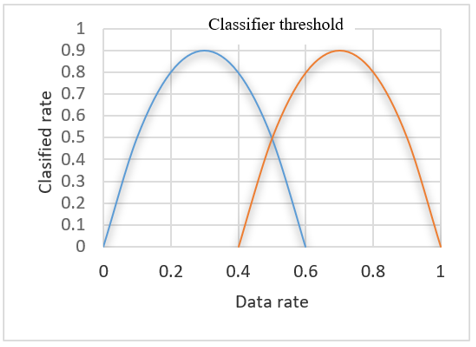
The confusion matrix is used to evaluate the accuracy of the model in the classification results. As can be seen in Figure 15 and Figure 16, the TN, TP, FN, FP values may change depending on the location of the threshold selected by the classifier.
Table 3. Results of the evaluation parameters
|
|
Accuracy |
Specificity |
Sensitivity |
|
Kernel |
0.8044 |
0.8311 |
0.7778 |
|
SVM |
0.7678 |
0.7467 |
0.7889 |
|
Naive Bayes |
0.8133 |
0.7622 |
0.8644 |
|
Ensemble |
0.7978 |
0.7689 |
0.8267 |
|
Tree |
0.7478 |
0.7311 |
0.7644 |
Figure 15. TN (True Negatif), TP (True Positif), FN (False Negatif), FP (False Positif) values in the classification of data according to a threshold
Figure 16. Confusion matrix, Predicted class vs. True class. EXCIT: excitatory, INHIB: Inhibitory
The accuracy in the confusion matrix is calculated as follows:
$\begin{aligned} \text { Accuracy }=&((\mathrm{TP}+\mathrm{TN}) /(\mathrm{TP}+\mathrm{TN}+\mathrm{FP}+\mathrm{FN})) \times 100 \\ &=\left(1-\frac{\text { misclassified }}{\text { total }}\right) \times 100 \end{aligned}$ (7)
The confusion matrix helps to identify areas where the classifier is malfunctioning. In the table, the rows show the actual class and the columns show the predicted class. Diagonal cells show how well the actual and predicted classes match.
Sensitivity $=\mathrm{TP} /(\mathrm{TP}+\mathrm{FN})$ (8)
Specificity $=\mathrm{TN} /(\mathrm{TN}+\mathrm{FP})$ (9)
4.1 Results
In this study, the Inter-Spike interval values of each neuronal sequence were converted to a recurrence plot image, the image features were extracted by Alexnet CNN and the classification of nerve cell types in the frontal cortex was performed in rats. In the study, classification methods such as kernel classification, support vector machines, Naive Bayes, Ensemble, decision tree were used. Results can be obtained with the data from the confusing matrices in Figures 17-19. The precision, sensitivity and specificity of the proposed methods were measured as evaluation parameters.
As can be seen in Table 3, the method that gave the best classification result was Naive Bayes with an accuracy of 81.33%, specificity of 76.22% and sensitivity of 86.44%. The best specificity value was obtained by Kernel classification with 83.11%. But its accuracy value is also important, but slightly lower than Naive Bayes. For the sensitivity, the result is among the lowest. With the best accuracy, after Naïve Bayes, we can use Kernel (80.44%) and Ensemble (79.78%) classifications. We can adopt the Naïve Bayes and Kernel classification for this work. The least suitable classifications are SVM and Tree.
Figure 17. Kernel classification confusion matrix. TP=350; FN=100; FP=76; TN=374
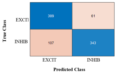
Figure 18. Naive Bayes confusion matrix. TP=389; FN=61; FP=107; TN=343
This algorithm gave the most effective result in the Ensemble trial with the Bag method.
Figure 19. Ensemble confusion matrix. TP=372; FN=78; FP=104; TN=346
Table 4. Best test result with the hyperparameter optimisation
|
|
Value of the objective function |
Function evaluation time (seconds) |
|
Kernel |
0.2176 |
175.9 |
|
SVM |
0.2390 |
15.1 |
|
Naive Bayes |
0.2081 |
273.41 |
|
Ensemble |
0.2005 |
352.4 |
|
Tree |
0.2452 |
23.81 |
In the hyperparameter optimization study, 30 trials were conducted for each method. The best results of the trials are presented in Table 4 according to different classification methods. Considering the evaluation time, we have seen the most optimal values with Kernel classification. Looking at the optimization results on Table 4, we can see that the Kernel classification is the most suitable. In kernel classification, an optimization study was carried out to find the best hyperparameters. With 30 trials, the value of the estimated and observed minimum objective function was 0.22. Using the kernel scaling parameter, a random basis for the extension of random features was obtained, which was at best 44,813. Lambda determines the power of regularity and was estimated to be 0.00018685 at best.
The most interesting function evaluation time is obtained by SVM, with 15.1 seconds. But with this, the value of the objective function remains relatively high (0.2390), which makes this algorithm less usable. The most interesting value of the objective function is obtained by Ensemble but with a very high function evaluation time (352.4 seconds). Considering both values, we can adopt the Kernel classification with a value of the objective function of 0.2176 and a function evaluation time of 175.9 seconds.
The classification of excitatory cells was, at best, obtained by Naive Bayes with 86.4%. The classification of inhibitory cells, on the other hand, was obtained by Kernel classification with 83.2% (Table 5).
Table 5. Results of classification of excitatory and inhibitory cells (%)
|
|
Excitator cell classification |
Inhibitor cell classification |
|
Kernel |
77.8% |
83.2% |
|
SVM |
78.9% |
74.7% |
|
Naive Bayes |
86.4% |
76.2% |
|
Ensemble |
82.7% |
76.9% |
|
Tree |
76.44% |
73.11% |
With the Kernel classification of inhibitor cells, the best result is obtained with 83.2%, but for excitator cells, this classification is 77.8%. The classification of excitator cells is maximal using Naive Bayes (86.4%) but this classification remains a bit weak for inhibitor cells (76.2). The classification of excitatory cells is also relatively interesting with Ensemble as we have obtained 82.7%. Ensemble gave us a slightly higher classification result for inhibitor cells than what we obtained with Naive Bayes. In this framework, the poorest results were given by SVM and Tree classification.
4.2 Discussion
Statistics and machine learning models did not obtain a very good classification of excitatory and inhibitory neurons, with data from the frontal cortex of the brain in the sleep and wakeful state in rats. The deep learning methods, which have not been used before with this type of data, allowed to have a classification with better results.
The classification of excitatory and inhibitory cells with only spike times sequences was performed by deep learning, without knowing all the properties of the raw signals (spike width, spike trough-peak length) and the intercellular interactions. More than 81% accuracy was obtained with respect to the Ground Truth. The best classification of excitatory cells was obtained by Naive Bayes with 86.4%. The best classification of inhibitory cells was obtained by Kernel classification with 83.2%. Using the same data set, but with more data, Lazarevich et al. [12] in their article "Neural activity classification with machine learning models on inter-spike interval series data", had found 65% success in classifying excitatory and inhibitory cells with machine learning methods. Compared to this value, we obtained better success with deep learning methods. We have also seen that we can reduce the number of data, and therefore the processing time to get a good classification result. Thus, it has been observed that cells can be classified as either excitatory or inhibitory with great success using spike time series that do not contain all the characteristics with respect to the raw waveform, and this with less data.
Although the success (> 90%) obtained with the raw wave based classification method cannot be achieved [3], these values are not far off. Consequently, the importance of temporal structure in neural data has been revealed. Under these conditions, we can say that such results are relatively important for neuroscientists.
If our data were raw spike trains, we believe our success rate could increase. Like Saif-ur-Rehman et al. [24] with the application of SpikeDeeptector, the classification study to distinguish between noise and signal from raw neural signals had 98.9% success with deep learning.
This dataset, which includes spike firing rate or time coding, made it possible to consider the temporal structure in an individual cell. The analysis of the fine temporal structure in the sequences was used to find the properties of the cells. It was observed that frontal cortex spike activity and classification of neuron types can be understood by spike times coding. We can say that the ISI properties of spike trains can carry information about the cell type and thus about the neural network activity.
In neural coding, recurrence plot images using ISI values have increased the success of classification. Recurrence plot was used to extract dynamic properties (dynamics, synchronization, regime changes) from the spike sequence data of these complex systems [38]. Lin et al. [29] in his work "Evaluation of vertical ground reaction forces pattern visualization in neurodegenerative diseases identification using deep learning and recurrence plot image feature extraction", Garcia-Ceja et al. [30] in his book "Classification of recurrence plots 'distance matrices with a convolutional neural network for activity recognition", Afonso et al. [31] in his study entitled "A recurrence plot-based approach for Parkinson's disease Identification", we saw the improvement of results thanks to recurrence plot and deep learning methods. We have shown that the same methods increase the success of our own study.
Recognizing the excitatory or inhibitory properties of nerve cells in a particular area of the brain, during sleep and wakefulness, helps to understand how individual cells interact and thus provides information about the "learning" of the neural network [14]. Concrete links have been established between neural network learning and spike-timing, which depends on plasticity [51]. It is promising to use deep learning methods to study learning in sleep and wakefulness with spike timing data.
It can be said that the representations learned through deep learning are used to better understand the structure of neuronal information. In this study, convolutional neural networks are used to better understand the activity of brain nerve cells. The results may help to understand the inspired model and to update its architecture.
In this study, the Inter-Spike interval values of the individual neuron spike sequence were converted into a recurrence plot image, the characteristics of the image were extracted using the pre-trained Alexnet learning transfer method and the classification of nerve cell types of the frontal cortex was performed. In our study, classification methods such as kernel classification, support vector machines, Naive Bayes, Ensemble, and finally the decision tree were used. More than 81% success was obtained with Naive Bayes in the classification of excitatory and inhibitory cells with temporal spike sequences, from which some wave properties and intercellular interaction information were suppressed. Thus, the cell type is defined automatically. It has been observed that the ISI properties of spike trains can carry information on cell type and thus neural network activity. Learning whether cells are excitatory or inhibitory indicates how individual cells interact. Consequently, the importance of temporal structure in neuronal data was revealed. Under these circumstances, these values are significant and important for neuroscientists.
In summary, deep learning neural network models help us, in part, to understand the neural networks of the brain. With these models, the temporal structure can be used without all the characteristics of the neural signal. As in the brain, in the execution of the model in question, we were able to process little data to obtain the required information.
In this study, we have seen the applicability of the methods used. In another study, we plan to do a more complete study and comparison using various trained networks, increasing the amount of data, modifying the pre-processing steps.
[1] Nörobilim. Nörobilim nedir? https://norobilim.com/norobilim-nedir/, accessed on 2014.
[2] The Brain Bank North West. Neural coding 1: How to understand what a neuron is saying? https://thebrainbank.scienceblog.com/2017/02/26/neural-coding-1-how-to-understand-what-a-neuron-is-saying, accessed on Feb. 26, 2017.
[3] Watson, B.O., Levenstein, D., Greene, J.P., Gelinas, J.N., Buzs´aki, G. (2016). Network homeostasis and state dynamics of neocortical sleep. Neuron, 90(4): 839-852. https://doi.org/10.1016/j.neuron.2016.03.036
[4] Watson, B., Levenstein, D., Greene, J.P., Gelinas, J.N., Buzsáki, G. (2016). Multi-unit spiking activity recorded from rat frontal cortex (brain regions MPFC, OFC, ACC, and M2) during wake-sleep episode wherein at least 7 minutes of wake are followed by 20 minutes of sleep. CRCNS. org, 10: K02N506Q. http://dx.doi.org/10.6080/K02N506Q
[5] Livezey, J.A., Glaser, J.I. (2020). Deep learning approaches for neural decoding: From CNNs to LSTMs and spikes to fMRI. arXiv. https://arxiv.org/pdf/2005.09687.pdf.
[6] Strosky, P.N. Brain-Machine Interface. Electrical Library. https://www.electricalelibrary.com/en/2019/03/22/brain-machine-interface/, accessed on March 22, 2019.
[7] Lefebvre, B., Yger, P., Marre, O. (2018). Recent progress in multi-electrode spike sorting methods. Journal of Physiology-Paris, 110(4): 327-335. https://doi.org/10.1016/j.jphysparis.2017.02.005
[8] Brown, E.N., Kass, R.E., Mitra, P.P. (2004). Multiple neural spike train data analysis: State-of-the-art and future challenges. Nature Neuroscience, 7(5): 456-461. https://doi.org/10.1038/nn1228
[9] Pachitarin, M., Steinmetz, N., Kadir, S., Carandini, M., Harris, K. (2016). Fast and accurate spike sorting of high-channel count probes with Kilosort. Conference on Neural Information Processing Systems 29.
[10] Rey, H.G., Pedreira, C., Quiroga, R.Q. (2015). Past, present and future of spike sorting techniques. Brain Research Bulletin, 119(Part B): 106-117. https://doi.org/10.1016/j.brainresbull.2015.04.007
[11] De Schutter, E. (2018). Deep Learning and Computational Neuroscience. Neuroinformatics, 16: 1-2. https://doi.org/10.1007/s12021-018-9360-6
[12] Lazarevich, I., Prokin, I., Gutkin, B. (2020). Neural activity classification with machine learning models on inter-spike interval series data. arXiv: 1810.03855v2.
[13] The University of Queensland. Queensland Brain Institute. What are Neurotransmitters? https://qbi.uq.edu.au/brain/brain-physiology/what-are-neurotransmitters, accessed on Nov. 9, 2017.
[14] Brendel, W., Bourdoukan, R., Vertechi, P., Machens, C.K., Deneve, S. (2020). Learning to represent signals spike by spike. Plos Computational Biology, 16(3): e1007692. https://doi.org/10.1371/journal. pcbi.1007692
[15] Basic physiology. Basic physiology Contents. http://basicphysiology.com/, accessed on Mar. 14, 2021.
[16] Tezuka, T. (2018). Multineuron spike train analysis with r-convolution kernel. Neural Networks, 102: 67-77. https://doi.org/10.1016/j.neunet.2018.02.013
[17] Li, M., Zhao, F., Wang, D., Kuang, H., Tsien, J.Z. (2015). Computational classification approach to profile neuron subtypes from brain activity mapping data. Scientific Reports, 5: 12474. https://doi.org/10.1038/srep12474
[18] Fang, H., Wang, Y., He, J. (2010). Spiking neural networks for cortical neuronal spike train decoding. Neural Computation, 22(4): 1060-1085. https://doi.org/10.1162/neco.2009.10-08-885
[19] Hirata, Y., Lang, E.J., Aihara, K. (2014). Recurrence Plots and the Analysis of Multiple Spike Trains. Springer Handbook of Bio-/Neuroinformatics, 735-744. https://doi.org/10.1007/978-3-642-30574-0_42
[20] Glaser, J.I., Benjamin, A.S., Chowdhury, R.H., Perich, M.G., Miller, L.E., Kording, K.P. (2020). Machine learning for neural decoding. eNeuro, 7(4): 0506-19. https://doi.org/10.1523/ENEURO.0506-19.2020
[21] Şeker, A., Diri, B., Balık, H.H. (2017). Derin öğrenme yöntemleri ve uygulamaları hakkında bir inceleme. Gazi Mühendislik Bilimleri Dergisi, 3(3): 47-64.
[22] Hinton, G.E., Dayan, P., Frey, B.J., Neal, R.M. (1995). The wake-sleep algorithm for unsupervised neural networks. Science, 268(5214): 1158-1161. https://doi.org/10.1126/science.7761831
[23] Chagas, A.M., Theis, L., Sengupta, B., Stüttgen, M.C., Bethge, M., Schwarz, C. (2013). Functional analysis of ultra high information rates conveyed by rat vibrissal primary afferents. Frontiers in Neural Circuits, 7: 190. https://doi.org/10.3389/fncir.2013.00190
[24] Saif-ur-Rehman, M., Lienkämper, R., Parpaley, Y., Wellmer, J., Liu, C., Lee, B., Kellis, S., Andersen, R., Iossifidis, I., Glasmachers, T., Klaes, C. (2019). SpikeDeeptector: A deep learning based method for detection of neural spiking activity. Journal of Neural Engineering, 16(5): 056003. https://doi.org/10.1088/1741-2552/ab1e63
[25] Jouty, J., Hilgen, G., Sernagor, E., Hennig, M.H. (2018). Non-parametric physiological classification of retinal ganglion cells in the mouse retina. Frontiers in Cellular Neuroscience, 12: 481. https://doi.org/10.3389/fncel.2018.00481
[26] Markanday, A., Bellet, J., Bellet, M.E., Hafed, Z.M., Thier, P. (2020). Using deep neural networks to detect complex spikes of cerebellar Purkinje cells. Neurophysiol., 123(6): 2217-2234. https://doi.org/10.1152/jn.00754.2019
[27] Racz, M., Liber, C., Nemeth, E., Fiath, R., Rokai, J., Harmati, I., Ulbert, I., Marton, G. (2019). Spike detection and sorting with deep learning. Journal of Neural Engineering, 17(1): 016038. https://doi.org/10.1088/1741-2552/ab4896
[28] Livezey, J., Glaser, J.I. (2018). Deep learning approaches for neural decoding: From CNNs to LSTMs and spikes to fMRI. arXiv:2005.09687.
[29] Lin, C., Wen, T., Setiawan, F. (2020). Evaluation of vertical ground reaction forces pattern visualization in neurodegenerative diseases identification using deep learning and recurrence plot image feature extraction. Sensors, 20(14): 3857. https://doi.org/10.3390/s20143857
[30] Garcia-Ceja, E., Uddin, M.Z., Torresen, J. (2018). Classification of recurrence plots’ distance matrices with a convolutional neural network for activity recognition. Procedia Computer Science, 130: 157-163. https://doi.org/10.1016/j.procs.2018.04.025
[31] Afonso, L.C.S., Rosa, G.H., Pereira, C.R., Weber, S.A.T., Hook, C., Albuquerque, V.H.C., Papa, J.P. (2018). A recurrence plot-based approach for Parkinson’s disease Identification. Future Generation Computer Systems, 94: 282-292. https://doi.org/10.1016/j.future.2018.11.054
[32] Fakı, B.M. (2015). Veri Madenciliği Yöntemlerini Kullanarak Anemi Sınıflandırmasına Yönelik Bir Uygulama. Yüksek Lisans Tezi, Istanbul Teknik Universitesi.
[33] Naselaris, T., Prenger, R.J., Kay, K.N., Oliver, M., Gallant, J.L. (2009). Bayesian reconstruction of natural images from human brain activity. Neuron, 63(6): 902-915. https://doi.org/10.1016/j.neuron.2009.09.006
[34] Cadena, S.A., Denfield, G.H., Walker, E.Y., Gatys, L.A., Tolias, A.S., Bethge, M., Ecker, A.S. (2019). Deep convolutional models improve predictions of macaque V1 responses to natural images. Plos Computational Biology, 15(4): e1006897. https://doi.org/10.1371/journal.pcbi.1006897
[35] NP Istanbul Beyin Hastanesi. Nörobilim Uygulama. https://npistanbul.com/norobilim-yuksek-lisansta-uygulama-firsati/1975, accessed on Jan. 13, 2017.
[36] Teeters, J.L., Sommer, F.T. (2009). Crcns. org: A repository of high-quality data sets and tools for computational neuroscience. BMC Neuroscience, 10: S6. https://doi.org/10.1186/1471-2202-10-S1-S6
[37] Eckmann, J.P., Kamphorst, S.O., Ruelle, D. (1995). Recurrence plots of dynamical systems. World Scientific Series on Nonlinear Science Series A, 16: 441-446.
[38] Goswami, B. (2019). A brief introduction to nonlinear time series analyses and recurrence plots. Vibration, 2(4): 332-368. https://doi.org/10.3390/vibration2040021
[39] Hassabis, D., Kumaran, D., Summerfield, C., Botvinick, M. (2017). Neuroscience-inspired artificial intelligence. Neuron, 95: 245-258. https://doi.org/10.1016/j.neuron.2017.06.011
[40] Storrs, K.R., Kriegeskorte, N. (2019). Deep Learning for Cognitif Neuroscience. arXiv,2019.
[41] Scherer, D., Müller, A., Behnke, S. (2010). Evaluation of pooling operations in convolutional architectures for object recognition. Artificial Neural Networks-ICANN, 2010: 92-101.
[42] CS231n Convolutional Neural Networks for Visual Recognition. Convolutional Neural Networks (CNN/ConvNets). https://cs231n.github.io/convolutional-networks/#fca, accessed on June 2, 2021.
[43] Graham, B. (2014). Fractional Max pooling. arXiv: 1412.6071v4.
[44] Springenberg, J.T., Dosovitskiy, A., Brox, T., Riedmiller, M. (2015). Striving For Simplicity: The All Convolutional Net. arXiv:1412.6806v3.
[45] Krizhevsky, A., Sutskever, I., Hinton, G.E. (2012). Imagenet classification with deep convolutional neural networks. Adv. Neural Inf. Process. Syst., 60(6): 84-90.
[46] Yakupoğlu, Y. (2018). Eğitimsel Veri Madenciliği Ve Bir Uygulaması. Yüksek Lisans Tezi, Istanbul Teknik Universitesi.
[47] Ali, A. (2018). Decision Tree (CART) Algorithm in Machine Learning. Wavy Al Reserch Fondation, Chapter 4.
[48] Takcı, H. (2016). Centroid Sınıflayıcılar Yardımıyla meme kanseri teşhisi. Journal of the Faculty of Engineering and Architecture of Gazi University Cilt, 31(2): 323-330.
[49] Bulut, F. (2017). Örnek tabanlı sınıflandırıcı topluluklarıyla yeni bir klinik karar destek istemi. Journal of the Faculty of Engineering and Architecture of Gazi University, 32(1): 65-76.
[50] Towards Data Science. Kernel Functions. https://towardsdatascience.com/kernel-function-6f1d2be6091, accessed on Jan. 2, 2017.
[51] Mathworks. fitckernel. https://fr.mathworks.com/help/stats/fitckernel.html, accessed on June 2, 2021.