Siva Priyanka S* | Kishore Kumar T
© 2021 IIETA. This article is published by IIETA and is licensed under the CC BY 4.0 license (http://creativecommons.org/licenses/by/4.0/).
OPEN ACCESS
In speech communication applications such as teleconferences, mobile phones, etc., the real-time noises degrade the desired speech quality and intelligibility. For these applications, in the case of multichannel speech enhancement, the adaptive beamforming algorithms play a major role compared to fixed beamforming algorithms. Among the adaptive beamformers, Generalized Sidelobe Canceller (GSC) beamforming with Least Mean Square (LMS) Algorithm has the least complexity but provides poor noise reduction whereas GSC beamforming with Combined LMS (CLMS) algorithm has better noise reduction performance but with high computational complexity. In order to achieve a tradeoff between noise reduction and computational complexity in real-time noisy conditions, a Signed Convex Combination of Fast Convergence (SCCFC) algorithm based GSC beamforming for multi-channel speech enhancement is proposed. This proposed SCCFC algorithm is implemented using a signed convex combination of two Fast Convergence Normalized Least Mean Square (FCNLMS) adaptive filters with different step-sizes. This improves the overall performance of the GSC beamformer in real-time noisy conditions as well as reduces the computation complexity when compared to the existing GSC algorithms. The performance of the proposed multi-channel speech enhancement system is evaluated using the standard speech processing performance metrics. The simulation results demonstrate the superiority of the proposed GSC-SCCFC beamformer over the traditional methods.
multi-channel speech enhancement, generalized sidelobe canceller (GSC) beamforming, adaptive filters, fast convergence normalized least mean square (FCNLMS), signed convex combination of fast convergence (SCCFC)
In multi-microphone array processing, environmental noise degrades the desired speech quality and intelligibility. This is a major issue in speech communication applications like teleconferences, mobile phones, etc. When the desired speaker is non-stationary [1], i.e., in a real-time noisy environment, reducing the noise becomes quite difficult. In these cases, for noise reduction and interference suppression [2], in the place of conventional Finite Impulse Response (FIR) filters which result in high computational complexities, the adaptive filters like, Least Mean Square (LMS), Normalized LMS (NLMS) are widely used for noise reduction. However, in the case of single-channel speech enhancement, noise from a specific direction cannot be found using these basic adaptive filters. So, in multi-channel speech enhancement, Griffiths and Jim [3] introduced a GSC beamforming structure that comprises three major blocks: fixed beamformer, blocking matrix, and an adaptive filtering block. In the fixed beamformer such as Delay and Sum Beamformer (DSB) [4], the microphone array receives the desired speech along with the noise. Delay from each microphone is calculated and then summed together to obtain the partially enhanced output [5, 6].
The performance of a multi-channel speech enhancement system depends completely on the blocking matrix and the adaptive filtering [7] block, which eliminates the unwanted noise and increases the quality of the desired speech. The adaptive filter block in the GSC beamforming plays a crucial role in noise reduction performance [8]. In the time domain, the gradient descent adaptive algorithms are used to update the weight of the filter. One such algorithm is the LMS algorithm which has low computational complexity but not stable in real-time noisy conditions when the filter tap gets increased [9-11]. Another popular adaptive algorithm is Recursive Least Squares (RLS) filter which is based on Hessian adaptive filtering. It gives faster convergence when compared to LMS whereas computational cost is high and is too expensive for real-time noisy environments [12, 13]. Fast convergence [14] algorithm has less computational complexity but gives less performance under various noisy conditions. And also when the positions of the source signal changes, the weight coefficient information used to update the adaptive filter will be lost, due to this, poor performance in the non-stationary environment combined adaptive filter [15-17] are designed, which give good convergence transition compared to the single adaptive filter.
To improve the adaption performance, adaptive beamforming with an Affine Projection Algorithm [18] (APA) is introduced, which gives a better noise reduction when compared to the existing time-domain algorithms but fails in the case of a real-time noisy environment. In the combined adaptive beamforming method [19], a combination of LMS-RLS adaptive filters in sidelobe canceller fails in real-time noisy conditions, and the computational burden is raised due to the mixing parameter. Another existing algorithm for noise reduction in recent times is, GSC beamformer with linear prediction filter [20] which is used in multichannel speech enhancement system addresses dereverberation and noise reduction, but has high computation complexity. Barnov et al., in 2019 introduced GSC beamforming using controlled white Gaussian gain [21], where non-stationary environments are only limited to a single speaker. A modified change prediction [22] to GSC beamforming is applied which holds good for echo cancellation but fails in interference suppression.
The above-mentioned algorithms give the motivation for the further improvement of the sidelobe canceller path of the GSC beamformer to achieve both noise reduction and less computational burden. To overcome these drawbacks, a robust beamforming method should be designed. In this paper, a GSC beamformer with SCCFC adaptive filters is proposed to address the above-mentioned issues. The novelty of the paper lies in the sidelobe cancelling path. In this paper, novelty is achieved in two steps. The first step is to consider FCNLMS as an adaptive filter in the convex combination algorithm to give a better noise reduction and a low computational complexity. The second step is to employ a signed algorithm, to further reduce the computational complexity in the mixing parameter design. In this way, using the signed algorithm with a convex combination of FCNLMS adaptive filters, both noise reduction, and low computational complexity are achieved under various real-time noisy conditions. The proposed GSC beamforming using the SCCFC algorithm shows better noise reduction and lower computation complexity when compared to the existing algorithms.
The main contributions of the work are as follows:
The paper is structured as follows: In Section 2 the proposed multi-channel speech enhancement system is described. In Section 3, the Signed Convex Combination of Fast Convergence (SCCFC) adaptive algorithm is discussed besides the description of the signed algorithm. The simulation environment and performance evaluation of the proposed system is discussed in Section 4. Finally, the conclusions are summarized in Section 5.
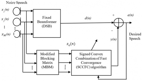
This section describes the multi-channel speech enhancement system in a real-time environment as shown in Figure 1. GSC beamformer comprises of three major blocks: a fixed beamformer and Modified Blocking Matrix (MBM) and a sidelobe cancelling path where an SCCFC is proposed. The input to the proposed system is considered using a microphone array setup with real-time noisy conditions in a virtual conference room.
The virtual conference room is designed based on the Image method [23] which takes the Room Impulse Response in the form of a Mex function in MATLAB. In this paper, DSB [10] is considered as a fixed beamformer.
Figure 1. Proposed multi-channel speech enhancement system using GSC-SCCFC
2.1 Fixed beamformer (DSB)
The DSB is used to find the direction of arrival (DOA) of the unknown signal. It calculates the DOA based on the delay and distance from each microphone. An unknown noisy input signal with partial enhancement is found at the output of DSB. To further reduce the noise in the signal, we proposed an SCCFC in the sidelobe cancelling path of the GSC beamformer. The required steps involved in the overall design of the GSC beamformer with the proposed SCCFC is explained below.
A microphone array with M microphones is considered in which xk(n) is the received signal by the kth microphone where k=1, 2, ..., M. It holds a delayed copy of the desired speech S(n) combined with the room impulse response, Rk, and real-time environment noise, Ek(n). Using the DSB beamformer principle, the delay from each microphone is calculated and summed up, so that the output of DSB will be a partially enhanced speech.
This is referred to as a speech reference signal d(n).
$d\left( n \right)=\sum\limits_{k=1}^{M}{{{x}_{k}}\left( n \right)} =\sum\limits_{k=1}^{M}{\sum\limits_{l=0}^{N-1}{{{R}_{k}}\left( n \right)S\left( N-l-{{\tau }_{k}} \right)}}+{{E}_{k}}\left( n \right)$ (1)
The length of the input signal is given by N. Delay from the input signal to the kth microphone is given by τk. Next is about blocking matrix explained as follows
Griffiths [3] devised a standard blocking scheme based on the idea that "by summing the rows of a matrix, it becomes zero," when following the binary-valued Walsh function or similar patterns in a matrix. However, since the current matrix does not fully leverage spatial knowledge, we created a Modified Blocking Matrix (MBM), in which the number of columns in the matrix indicates the number of microphones.
2.2 Modified blocking matrix
The blocking matrix is very important in GSC beamforming. It is used to block the desired speech signal and only provide noise reference as input to the adaptive interference canceller, as stated below. The GSC beamformer's lower path contains a blocking matrix [3], which is used to block the desired signal d(n). Since the desired signal is the same for all microphones and in Eq. (1), blocking is verified if the blocking matrix's rows add up to nil.
If $b_{m}^{T}$ is the mth row of blocking matrix
$b_{m}^{T}1=0$ for all values of m
Since bm is linearly independent, zq(n) it will have M-1 linearly independent components. As a result, the blocking matrix's row dimensions must be M-1.
If we assume that there are four microphones, M=4. Griffiths [3] defined two blocking matrices.
The first is defined as follows:
$B{{M}_{1}}=\left[ \begin{matrix}1\\1\\1\\\end{matrix}\begin{matrix}1\\-1\\-1\\\end{matrix}\begin{matrix}-1\\-1\\1\\\end{matrix}\begin{matrix}-1\\-1\\1\\\end{matrix} \right]$
The second blocking matrix is similarly defined as
$B{{M}_{2}}=\left[ \begin{matrix}1\\0\\0\\\end{matrix}\begin{matrix}-1\\1\\0\\\end{matrix}\begin{matrix}0\\-1\\1\\\end{matrix}\begin{matrix}0\\0\\1\\\end{matrix} \right]$
The rows in BM1 are mutually orthogonal and are elements of a binary-valued Walsh equation, while the difference between adjacent microphone outputs is represented by BM2. BM1 has different amplitude responses for each row, while BM2 has the same patterns. However, the spatial information is not fully used when these matrices are used.
So, using adjacent microphones, the Modified Blocking Matrix (MBM) is designed to subtract the desired speech from the input noisy signal. By using similar patterns in the matrix, MBM is used in the proposed GSC beamformer to use full spatial information on adjacent microphones as well as on other microphones.
MBM is designed as
$\mathrm{MBM}=\left(\begin{array}{cccccc}1 & -1 & 0 & & 0 & 0 \\ 0 & 1 & -1 & \cdots & 0 & 0 \\ 0 & 0 & 0 & & 0 & 0 \\ & \vdots & & \ddots & & \vdots & \\ 0 & 0 & 0 & & -1 & 0 \\ 0 & 0 & 0 & \cdots & 0 & -1\end{array}\right)$
The number of columns in the matrix indicates the microphone here with q=1,..., Q where Q=M - 1, where M is the number of microphones.
MBM gives the details of the complete noise present in the target signal and blocks the desired speech and thus acts as noise reference for SCCFC.
These constraints are considered to show the effectiveness of the proposed SCCFC in the GSC structure. The noise reference signals are adapted using the proposed SCCFC algorithm. The error at the output of the GSC beamformer is the difference between SCCFC output y(n) and speech reference d(n). Then, the GSC-SCCFC beamformer output is given by e(n)=d(n)-y(n). The error is updated using the proposed SCCFC algorithm until it is minimized.
The derivation of the SCCFC algorithm is shown in the below section. Firstly, a convex combination of the FCNLMS adaptive filter is drawn and then the signed algorithm is applied using the transfer approach in the next section.
The proposed SCCFC block is a signed convex combination of two same fast convergence adaptive filters i.e., FCNLMS, as shown in Figure 2 with updating rule which is given by:
$H_{n,q}^{(l)}\in {{\mathbb{R}}^{N}}={{\left( h_{0,q}^{(l)}(n),h_{1,q}^{(l)}(n),.....h_{N-1,q}^{(l)}(n) \right)}^{T}}$ (2)
where, $H_{n,q}^{(l)}$ is the vector with qth filter coefficients of lthsystem, with l=a,b at nth time instant, l=a implies first FCNLMS filter and l=b second FCNLMS filter. qth noise reference vector is expressed similarly.
${{Z}_{n,q}}\in {{R}^{N}}={{\left( {{z}_{q}}\left( n \right){{z}_{q}}\left( n-1 \right)....{{z}_{q}}\left( n-N+1 \right) \right)}^{T}}$ (3)
The combined adaptive filter is obtained by combining the two adaptive filter outputs using the mixing parameter. y(l)(n) is the output of combined adaptive filter which is defined as
Figure 2. Proposed convex combination of fast convergence adaptive filter
${{y}^{(l)}}(n)=\sum\limits_{q=1}^{Q}{y_{q}^{(l)}(n)}$ (4)
The convex combination of y(a)(n) and y(b)(n) is given by
where, $\tilde{C}_{N}(n)$ is dual Kalman gain [14], γN(n) is the Likelihood variable [14].
Dual Kalman gain is defined as:
$y(n)=\lambda (n){{y}^{(a)}}(n)+(1-\lambda (n)){{y}^{(b)}}(n)$ (5)
where, λ(n) is a mixing parameter, and ranges from [0,1] [16]. When λ(n)=0 the small step size filter (slow filter) works effectively by maintaining low steady-state error. When λ(n)=1, the large step size filter (fast filter) works better with high convergence, to limit the λ(n) range between [0,1], the mixing parameter is expressed by sigmoid function and an auxiliary parameter I(n).
$\lambda (n)=\frac{1}{1+{{e}^{-I(n)}}}$ (6)
The convex combined filter [16] error is minimized by adapting I(n) and is defined as:
$I(n+1)=I(n)+{{\mu }_{I}}e(n)\left[ \begin{align} & {{y}^{(a)}}(n)-{{y}^{(b)}}(n) \\ \end{align} \right]\lambda (n)[1-\lambda (n)]$ (7)
To reduce the inactivity when λ(n) is equal to 0 or 1, the auxiliary parameter is limited to [-I+, I+], such that the mixing parameter is made to move in [1-λ+, λ+]. Here, I+ and λ+ are small positive constants. The update rule of the weight vector $H_{n,q}^{l}(n+1)$ for lth an adaptive filter (l=a,b) is written as
$H_{n,q}^{(l)}(n+1)=H_{n-1,q}^{(l)}-\mu e_{q}^{(l)}(n){{\gamma }_{N}}(n){{\tilde{C}}_{N}}(n)$ (8)
$\widetilde{C_{N}}(n)=-\frac{Z_{n, p}(n)}{\frac{\lambda}{1-\lambda} \sigma_{z}^{2}+c_{o}}$ (9)
where, co and λ is a small positive constant. Likelihood variable is defined as:
${{\gamma }_{N}}(n)=\frac{1}{1-\sum\limits_{k=1}^{N}{v(n-k+1)}}$ (10)
where, $v(n)=C_{N}^{(-1)}x(n)$ is the shifting component, $e_{q}^{(l)}(n)$ in Eq. (8). is the error estimator of FCNLMS filter with qth error signal, expressed as
$e_{q}^{(l)}=d(n)-y_{q}^{(l)}(n)$ (11)
where, $y_{q}^{(l)}(n)$ is the FCNLMS filter output of qth filter and is expressed as
$y_{q}^{(l)}(n)=Z_{n,q}^{T}H_{n-1,q}^{(l)}$ (12)
where, ${{\mu }_{l}}$ is the step size of lth adaptive filter.
The overall weight coefficient of the convex combination of the adaptive filters is expressed as
${{H}_{n,q}}=\lambda (n)H_{n,q}^{(a)}(n)+[1-\lambda (n)]H_{n,q}^{(b)}$ (13)
By updating the filter with the help of the mixing parameter, there is a decent trade-off between the convergence speed and steady-state error. However, such algorithms require fixing of mixing parameters while updating the weights resulting in the loss of information. Complexity burden increases due to I(n) in the update rule and also fails to work for real-time noises. To avoid these issues, a GSC beamformer for various real-time noise reductions with fewer operations in the I(n) update rule should be developed.
To overcome the computational burden on mixing parameters and overall real-time noise reduction. In this paper, a signed algorithm is proposed for the convex combination of fast convergence adaptive filters, which is described in the next section.
3.1 Signed algorithm to convex combination of fast convergence adaptive filters
We propose the SCCFC algorithm in this section. By opting for this signed algorithm, the mixing parameter update rule is changed to limit the squared estimation error.
$J(n)=\frac{1}{2}{{e}^{2}}(n)$ (14)
The gradient ${{\nabla }_{I}}J(n),$ is normalized and I(n), is updated recursively and is expressed as:
$I(n+1)=I(n)-{{\mu }_{I}}\frac{{{\nabla }_{I}}J(n)}{\parallel {{\nabla }_{I}}J(n)\parallel }$ (15)
Here ${{\mu }_{I}}$ is a step-size and is a small positive constant, ${{\nabla }_{I}}J(n),$ is defined as
${{\nabla }_{I}}J(n)=-e(n)({{y}_{a}}(n)-{{y}_{b}}(n))\lambda (n)(1-\lambda (n))$ (16)
The normalized gradient $\frac{{{\nabla }_{I}}J(n)}{\left\| {{\nabla }_{I}}J(n) \right\|}$ in Eq. (15). can be expressed as
$\frac{\nabla_{I} J(n)}{\left\|\nabla_{I} J(n)\right\|}=\operatorname{sgn}\left(\nabla_{I} J(n)\right)$ (17)
where, $\operatorname{sgn}(.)$ is a sign function [16] and is defined as
$\operatorname{sgn}(.)=\frac{u}{\|z\|}=\left\{\begin{array}{lll}1 & \text { if } & z>0 \\ 0 & \text { if } & z=0 \\ -1 & \text { if } & z<0\end{array} . \rightarrow\right.$ (18)
Therefore, Eq. (15). can be written as
$I(n+1)=I(n)+\mu_{I} \operatorname{sgn}\left(\begin{array}{l}e(n) y^{(a)}(n) \\ -y^{(b)}(n) \lambda(n)(1-\lambda(n))\end{array}\right)$ (19)
As λ(n)>0 & 1-λ(n)>0the parameter I(n) in Eq. (19). can also be represented as
$I(n+1)=I(n)+\mu_{I} \operatorname{sgn}\left(e(n)\left(y^{(a)}(n)-y^{(b)}(n)\right)\right)$ (20)
$I(n+1)=I(n)+\mu_{I} \operatorname{sgn}\left(e(n)\left(e^{(a)}(n)-e^{(b)}(n)\right)\right)$ (21)
The proposed SCCFC algorithm can reduce computational complexity and attain robustness by replacing $e(n)[{{y}^{(a)}}(n)-{{y}^{(b)}}(n)]\lambda [1-\lambda (n)]$ it with normalized gradient $\frac{\nabla_{I} J(n)}{\left\|\nabla_{I} J(n)\right\|}$.
To enhance the speech further with less computation, while maintaining high convergence, an instant transfer algorithm [16] can be used,
if nmod ${{D}_{o}}=0$ and $I(n+1)={{I}^{+}}$ then
$H_{n,q}^{(b)}(n+1)=H_{n,q}^{(a)}(n+1)$
endif
where, Do is the length of the window. During convergence transition, an instant transfer algorithm is applied only when the first FCNLMS is effective than the second FCNLMS filter. The computation cost of this algorithm is smaller compared to the traditional combination filters. Due to the predefined window length, the computation burden is still reduced so that, the proposed SCCFC works effectively for various real-time noises with low complexity in updating the adaptive filter.
Overall steps involved in the proposed SCCFC algorithm is summarized as follows
|
Summary of proposed SCCFC algorithm |
|
|
|
|
|
|
Signed Algorithm |
|
if |
|
$I(n+1)<-{{I}^{+}}$ |
|
$I(n+1)=-{{I}^{+}}$ $\lambda (n+1)=0$ |
|
endif if |
|
$I(n+1)\ge -{{I}^{+}}$ |
|
$\lambda (n+1)=1$ if$(\bmod (n-1),{{D}_{o}}=0)$ $H_{n,q}^{(b)}(n+1)=H_{n,q}^{(a)}(n)(n+1)$ endif |
|
else |
|
$H_{n,q}^{(b)}=H_{n-1,q}^{(b)}-\mu e_{q}^{(b)}(n){{\gamma }_{N}}(n){{\tilde{C}}_{N}}(n)$ |
|
${{H}_{n,q}}=\lambda (n)H_{n,q}^{(a)}(n)+[1-\lambda (n)]H_{n,q}^{(b)}$ endif |
|
let n=n+1 end |
The workflow of the proposed multi-channel speech enhancement system (GSC-SCCFC) is as shown in Figure 3.
Figure 3. Workflow of proposed multi-channel speech enhancement system (GSC-SCCFC)
Table 1. Computational complexity
|
Algorithms |
Multiplications |
Primary combinations |
Precise weight calculations |
Weight transfer |
|
LMS [11] |
2N+1 |
- |
- |
- |
|
NLMS [13] |
2N |
- |
- |
- |
|
FCNLMS [14] |
2N |
- |
- |
- |
|
CLMS [16] |
4N+2 |
6 |
2N |
2N |
|
SCCFC (proposed) |
4N |
3 |
2N |
- |
3.2 Computational complexity
The computational complexity of the LMS [11], NLMS [13], FCNLMS [14], CLMS [16], and the proposed SCCFC algorithms are compared in this section. Here the length of the adaptive algorithm is given by N. For a regular LMS algorithm takes 2N+1 multiplications to update the filter. The basic NLMS and FCNLMS algorithms require a 2N number of multiplications. The proposed SCCFC algorithm which is a combination of the two same filters FCNLMS requires 4N multiplications to update the filter components. According to Eq. (15). to update I(n) the proposed SCCFC required only 3 multiplications, whereas the existing CLMS algorithm requires 6 multiplications to update the same I(n) parameter. Due to the usage of the signed algorithm with known window length, the proposed SCCFC algorithm reduces the computational operations compared to the conventional algorithms. Coming to stability, the relative variations in e(n) is maintained by taking μ as a small positive constant. Also, the mixing parameter I(n) is independent on J(n), I(n) becomes more stable when the ${{\nabla }_{I}}J(n)$ is small.
Finally, the proposed GSC-SCCFC gives less computation complexity with 4N multiplications, where N=256 is the length of the filter and requires three primary combinations in the update rule which is very less compared to existing algorithms. The computational complexity of the proposed multi-channel speech enhancement system is compared with the existing algorithms as shown in Table 1. The proposed algorithm also gives good trade-off stability compared to the other algorithms.
In this section, the simulation of the proposed GSC-SCCFC in real-time noisy conditions is evaluated and explained. The proposed GSC-SCCFC method considers the following simulation parameter as shown in Table 2. A multi-channel room impulse response is generated using a Mex function in MATLAB (rir-generator.cpp [24]) taking the above specifications.
Table 2. Specification parameters
|
Parameters |
Specifications |
|
Number of microphones(m) |
m=4 |
|
Spacing to each microphone |
5cm |
|
Real-time noisy environment |
Car, Restaurant, Babble, Airport, Station, and Street |
|
Input SNR Levels |
-10 dB, -5 dB, 0 dB, 5 dB, 10 dB, 15 dB |
|
Room dimensions |
6 m X 5 m X 3 m (Image Method) [23] |
|
Database |
DARPA TIMIT [25] and Noizeus [26, 27] |
|
Tools |
MATLAB and Python |
|
Processor |
Intel Core I7 Processor, Clock Speed-2.20 GHz, 8 GB RAM |
The real-time noisy condition is created by adding desired speech and real-time noises from unknown directions. The desired speech is taken using the DARPA TIMIT [25] database. The database is maintained with a sampling frequency of 8 kHz which consists of 6300 male and female sentences where each of the 630 speakers speaks 10 sentences each. The real-time noises (Car, Restaurant, Babble, Airport, Station, Street noises) are taken from the NOIZEUS database [26, 27]. These input signals are provided to the mex setup which gives a combination of the desired speech with real-time noise for different SNRs (-10 dB to 15 dB).
The degraded speech is an input to the DSB to evaluate the delay from each microphone and obtains a reference enhanced signal. After that, the input degraded speech is given to MBM. Using the MBM matrix, the subtraction of the delays caused on the adjacent microphones is calculated. Further, at the MBM output, a noise reference is generated. Finally, the same reference noise is applied to the SCCFC block as input where the weights of the individual filters are updated and combined using a mixing parameter. Due to the proposed SCCFC algorithm, the error is minimized and enhanced speech is attained at the output of the GSC beamformer.
The proposed GSC-SCCFC algorithm is compared with different existing algorithms like Combined adaptive beamforming [19], GSC with improved linear prediction [20], GSC with controlled white Gaussian [21], combined beamforming and echo cancellation [22] which are represented as GSC-CC [2013], GSC-LP [2018], GSC-CWGN [2019], and GSC-CBE [2019] respectively. GSC-CC algorithm uses a combination of adaptive filters [LMS-RLS] for noise reduction. GSC-LP multichannel improve linear predictor to improves the spatial filter. Both GSC-CBE and GSC-CWGN are used for noise reduction under white noise.
4.1 Performance analysis of proposed GSC-SCCFC algorithm under various environmental noises
The performance of the proposed GSC-SCCFC algorithm is evaluated using standard speech processing performance metrics namely Perceptual Evaluation of Speech Quality [28] (PESQ), Segmental SNR (SSNR) [29], Log-Spectral Distance (LSD) [30], and Log-Likelihood Ratio [28].
4.1.1 PESQ
PESQ [28] is an objective comprehensible measure. The range of PESQ as per the Standards International Telecommunication Union Telecommunication (ITU-T) lies in between “0.5 to 4.5”. The more the PESQ, the better is the intelligibility. Table 3 shows the PESQ score comparison of GSC-SCCFC over existing methods. Under station noise, for -10 dB, the proposed GSC- SCCFC PESQ score is 3.302, but for GSC-CC it is 2.411. Similarly, at 15 dB input SNR for street noise, PESQ for the proposed GSC-SCCFC is 4.393 but for GSC-CWGN and GSC-CBE it is 3.401 and 3.567, respectively.
At -10 dB car noise, the proposed GSC-SCCFC method gives a PESQ of 2.632, but for GSC with CWGN and CBE, it is 2.305 and 2.401, respectively. Similarly, at 15 dB PESQ for GSC-CWGN, GSC-CBE, and the proposed GSC-SCCFC are 3.232, 3.451, and 4.365 respectively. Similarly, for the remaining noises too, the perception is improved for the enhanced speech using the proposed GSC-SCCFC algorithm when compared with conventional algorithms as shown in Table 3. For the proposed method, an improvement in PESQ of 4.393 is achieved, which is very much closer to the maximum PESQ that can be achieved. Due to SCCFC, at the output, the desired speech perception is attained.
4.1.2 SSNR
SSNR [29], SSNR is the renowned objective measure for speech enhancement. In SNR, the complete signal is taken into consideration whereas, for SSNR, the segments with 256 samples per frame are considered. (k=256, with 50 percent overlap). Higher the Segmental SNR, more will be the speech quality.
SSNR is defined as
$SSNR=\frac{10}{N}\frac{\sum\limits_{q=0}^{N-1}{10\log \sum\limits_{q=0}^{M-1}{{{z}^{2}}(q+\frac{nM}{2})}}}{\sum\limits_{q=0}^{M-1}{{{[(q+\frac{nM}{2})-e(q+\frac{nM}{2})]}^{2}}}}$ (22)
From Table 3 at -10 dB with car noise, SSNR for GSC-SCCFC algorithm is 11.2, but for GSC-CC, GSC-LP, GSC-CWGN, and GSC-CBE, it is 2.9, 3.7, 4.2, and 5.6 respectively. Similarly, SSNR for 15 dB GSC-SCCFC is 32.5 while that for GSC-CC, GSC-LP, GSC-CWGN, and GSC-CBE are 15.3, 16.2, 17.6, and 19.8 respectively. SSNR for the proposed GSC-SCCFC shows improved performance as noise present in each frame is reduced. Also for 15 dB station noise, SSNR for GSC-SCCFC is 33.8, but for GSC-CC, GSC-LP, GSC-CWGN, and GSC-CBE, it is 15.8, 15.9, 16.2, and 22.6 respectively. Likewise for 15 dB street noise, GSC-SCCFC, GSC-CC, GSC-LP, GSC-CWGN, and GSC-CBE results in SSNRs of 34.6, 16.2, 17.4, 18.4, and 22.1, respectively. Likewise, the performance of SSNR is improved gradually for different real-time noises which are represented in Table 3. SSNR for the proposed GSC-SCCFC with four microphones gives better noise reduction in the segmental analysis.
Table 3. Comparison of PESQ and SSNR of proposed GSC-SCCFC with existing methods
|
SNR in dB |
Noise Type |
GSC-CC [2013] |
GSC-LP [2018] |
GSC-CWGN [2019] |
GSC-CBE [2019] |
GSC-SCCFC (Proposed)
|
|||||
|
PESQ |
SSNR |
PESQ |
SSNR |
PESQ |
SSNR |
PESQ |
SSNR |
PESQ |
SSNR |
||
|
-10 |
Car |
2.401 |
2.9 |
2.482 |
3.7 |
2.305 |
4.2 |
2.401 |
5.6 |
2.632 |
11.2 |
|
-10 |
Restaurant |
2.325 |
4.6 |
2.062 |
4.9 |
2.232 |
5.8 |
2.591 |
5.9 |
3.013 |
15.3 |
|
-10 |
Babble |
2.303 |
2.8 |
2.123 |
4.2 |
2.200 |
5.2 |
2.501 |
6.1 |
3.022 |
16.1 |
|
-10 |
Station |
2.411 |
5.2 |
2.102 |
3.2 |
2.428 |
4.5 |
2.656 |
5.3 |
3.302 |
12.1 |
|
-10 |
Airport |
2.510 |
3.7 |
2.323 |
4.2 |
2.398 |
5.7 |
2.618 |
6.3 |
2.801 |
13.3 |
|
-10 |
Street |
2.241 |
4.4 |
2.208 |
5.5 |
2.511 |
6.2 |
2.674 |
7.7 |
3.011 |
16.7 |
|
-5 |
Car |
2.008 |
3.6 |
2.569 |
4.2 |
2.507 |
5.1 |
2.604 |
7.2 |
2.804 |
17.2 |
|
-5 |
Restaurant |
2.211 |
4.7 |
2.381 |
3.6 |
2.316 |
4.8 |
2.623 |
7.8 |
3.093 |
21.5 |
|
-5 |
Babble |
2.007 |
5.1 |
2.312 |
4.5 |
2.421 |
5.9 |
2.729 |
8.1 |
3.201 |
18.1 |
|
-5 |
Station |
2.118 |
3.5 |
2.421 |
3.8 |
2.551 |
6.7 |
2.634 |
8.4 |
3.104 |
16.8 |
|
-5 |
Airport |
2.092 |
2.8 |
2.383 |
4.1 |
2.483 |
6.2 |
2.715 |
9.4 |
3.302 |
15.2 |
|
-5 |
Street |
2.183 |
5.7 |
2.572 |
5.9 |
2.501 |
7.5 |
2.749 |
9.5 |
3.259 |
20.3 |
|
0 |
Car |
2.010 |
7.2 |
2.454 |
6.9 |
2.611 |
5.9 |
2.734 |
9.2 |
3.405 |
21.4 |
|
0 |
Restaurant |
2.486 |
3.1 |
2.687 |
7.3 |
2.643 |
6.4 |
2.787 |
8.5 |
3.401 |
25.3 |
|
0 |
Babble |
2.201 |
5.4 |
2.532 |
7.9 |
2.571 |
6.3 |
2.663 |
10.5 |
3.569 |
24.2 |
|
0 |
Station |
2.229 |
7.5 |
2.556 |
6.8 |
2.691 |
6.9 |
2.719 |
9.7 |
3.582 |
22.8 |
|
0 |
Airport |
2.237 |
4.6 |
2.399 |
8.1 |
2.582 |
7.1 |
2.697 |
10.6 |
3.691 |
21.5 |
|
0 |
Street |
2.597 |
6.9 |
2.573 |
7.9 |
2.660 |
8.2 |
2.793 |
11.5 |
3.710 |
25.2 |
|
5 |
Car |
2.602 |
8.8 |
2.735 |
9.3 |
2.812 |
9.5 |
2.867 |
10.7 |
3.408 |
21.7 |
|
5 |
Restaurant |
2.676 |
7.2 |
2.812 |
8.9 |
2.752 |
9.8 |
2.702 |
11.3 |
3.421 |
25.1 |
|
5 |
Babble |
2.698 |
5.8 |
2.790 |
9.5 |
2.862 |
10.2 |
2.923 |
11.7 |
3.543 |
24.2 |
|
5 |
Station |
2.702 |
4.7 |
2.809 |
10.2 |
2.951 |
10.7 |
2.921 |
12.1 |
3.521 |
22.6 |
|
5 |
Airport |
2.818 |
4.9 |
2.901 |
9.9 |
3.028 |
10.5 |
3.052 |
11.9 |
3.671 |
21.9 |
|
5 |
Street |
2.992 |
8.9 |
3.095 |
12.8 |
3.191 |
11.7 |
3.179 |
13.8 |
3.722 |
25.2 |
|
10 |
Car |
2.901 |
10.6 |
3.011 |
11.7 |
3.221 |
12.7 |
3.328 |
13.3 |
3.992 |
31.9 |
|
10 |
Restaurant |
2.822 |
12.4 |
3.039 |
11.6 |
3.219 |
13.7 |
3.222 |
13.5 |
4.072 |
32.4 |
|
10 |
Babble |
2.899 |
15.1 |
3.156 |
11.9 |
3.312 |
13.2 |
3.356 |
14.2 |
4.287 |
34.1 |
|
10 |
Station |
2.907 |
12.2 |
3.121 |
12.7 |
3.224 |
12.9 |
3.401 |
14.8 |
4.356 |
32.8 |
|
10 |
Airport |
2.974 |
13.2 |
3.111 |
11.6 |
3.212 |
13.2 |
3.456 |
14.1 |
4.456 |
34.1 |
|
10 |
Street |
3.012 |
14.7 |
3.223 |
15.6 |
3.431 |
16.3 |
3.582 |
17.7 |
4.311 |
31.6 |
|
15 |
Car |
3.061 |
15.3 |
3.151 |
16.2 |
3.232 |
16.3 |
3.451 |
19.8 |
4.365 |
32.5 |
|
15 |
Restaurant |
2.921 |
15.9 |
3.164 |
16.2 |
3.379 |
1.8 |
3.511 |
20.9 |
4.346 |
34.3 |
|
15 |
Babble |
3.056 |
15.2 |
3.178 |
15.4 |
3.245 |
16.9 |
3.489 |
20.3 |
4.310 |
34.1 |
|
15 |
Station |
3.110 |
15.8 |
3.208 |
15.9 |
3.212 |
16.2 |
3.501 |
22.6 |
4.355 |
33.8 |
|
15 |
Airport |
3.089 |
15.5 |
3.219 |
16.9 |
3.302 |
17.8 |
3.451 |
21.7 |
4.387 |
34.8 |
|
15 |
Street |
3.121 |
16.2 |
3.410 |
17.4 |
3.401 |
18.4 |
3.567 |
22.1 |
4.393 |
34.6 |
4.1.3 LSD
LSD [30], is an Advanced metric, the reduction in the spectral distance is calculated using LSD.
The expression LSD is provided in Eq. (23),
$LSD=\frac{10}{N}\sum\limits_{n=0}^{(N-1)}{\frac{1}{(M+1)}}\sum\limits_{n=0}^{(\frac{M}{2})}{{{[\log {{z}_{q}}(n)-\log e(n)]}^{2}}}$ (23)
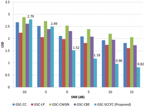
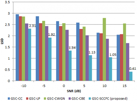
LSD for the proposed GSC-SCCFC algorithm is compared with existing algorithms for various real-time noises as shown in Figure 4a to 4f. The proposed algorithm showing lower values of LSD implies better performance. The reduction of the spectral distance is achieved using MBM by utilizing the complete spatial information. As the distance between the frames decreases, the distortion gets reduced. At 10 dB for car noise, LSD for GSC-SCCFC is 0.91 but for GSC-CC, GSC-LP, GSC-CWGN, and GSC-CBE, it is 2.04, 2.22, 2.39, 2.21. For 15 dB input SNR under station noise, LSD for GSC-SCCFC, GSC-CC, GSC-LP, GSC-CWGN, and GSC-CBE is 0.51, 1.54, 2.16, 2.03, and 1.73, respectively. The proposed GSC-SCCFC achieves better performance when compared to the existing algorithms. LSD gradually decreases for the remaining noises which are shown in Figure 4. A smaller spectral distance for the proposed GSC-SCCFC for 15 dB at 0.41 is observed under street noise. Using the proposed SCCFC algorithm in the adaptive filtering block of GSC beamforming, better quality is achieved for the output speech which is represented in terms of LSD as shown in Figure 4a to 4f.
a. LSD for airport noise
b. LSD for babble noise
c. LSD for car noise
d. LSD for restaurant noise
e. LSD for station noise
f. LSD for street noise
Figure 4. LSD comparison for proposed GSC-SCCFC with existing method under various noisy conditions
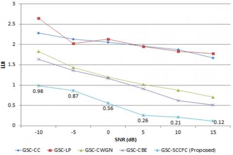
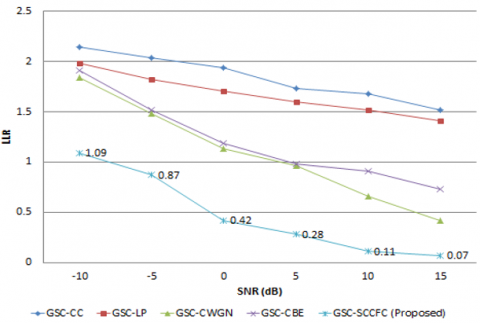
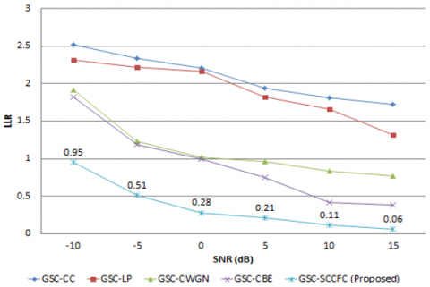
4.1.4 LLR
LLR [28] is an objective measure defined based on the LPC co-efficient, where αc is the LPC vector of clean speech and αp is the LPC vector of the processed speech and Rc is the auto-correlation matrix of the clean speech.
LLR can be calculated as
${{d}_{LLR}}({{\alpha }_{p}},{{\alpha }_{c}})=\log \left( \frac{{{\alpha }_{p}}{{R}_{c}}\alpha _{p}^{T}}{{{\alpha }_{c}}{{R}_{c}}\alpha _{c}^{T}} \right)$ (24)
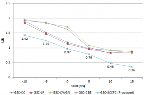
Lower the LLR more will be speech performance quality. For car noise at 15 dB input SNR, LLR is 0.36 for the proposed GSC-SCCFC, but for GSC-CC, GSC-LP, GSC-CWGN, and GSC-CBE it is 0.89, 0.87, 0.83, and 0.72, respectively. For station noise with 15 dB input SNR, GSC-SCCFC results in an LLR of 0.07 whereas GSC-CC, GSC-LP, GSC-CWGN, and GSC-CBE, it is 1.52, 1.41, 0.42, and 0.73 respectively. At 15 dB input SNR, LLR of 0.04 under airport noise is achieved by the proposed GSC-SCCFC which is very low when compared to the other conventional algorithms as shown in Figure 5a to 5f.
a. LLR for airport noise
b. LLR for babble noise
c. LLR for car noise
d. LLR for restaurant noise
e. LLR for station noise
f. LLR for street noise
Figure 5. LLR comparison for proposed GSC-SCCFC with existing method under various noisy conditions
Table 4. Computation time
|
Methods |
Computation time (s) |
|
GSC-CC [2013] |
2.38 |
|
GSC-LP [2018] |
1.98 |
|
GSC-CWGN [2019] |
2.71 |
|
GSC-CBE [2019] |
2.29 |
|
GSC-SCCFC (proposed) |
0.93 |
4.2 Computational time
The computational time is calculated in this section. An input degraded speech signal from the real-time environment with a duration of 2.814 seconds is considered. The simulations are executed on an intel i7 core processor with a 2.20 GHz clock speed with 8 GB RAM. The operating system used is Windows 10. The GSC-SCCFC is compared with the conventional algorithm in Table 4. GSC-SCCFC shows less computation of 0.93 s is shown in Table 4. The conventional algorithm shows low performance in noise reduction and gives high computation time is shown in Table 4. The proposed GSC-SCCFC method gives better performance with lower computational time.
4.3 Waveforms
In Figure 6 and Figure 7, the time domain plots and spectrograms of the proposed multi-channel speech enhancement system are illustrated. Which shows the proposed GSC-SCCFC noise reduction performance for 5 dB car noise. The enhanced speech signal of the proposed GSC-SCCFC algorithm shown in Figure 6 looks similar to the clean speech signal. The enhanced speech signal is also attained at low SNRs.
Figure 6. The time-domain plot of the proposed multi-channel speech enhancement system
Figure 7. Spectrogram of the proposed multi-channel speech enhancement system
Using the proposed GSC-SCCFC method, PESQ of 4.393 is obtained which is the highest compared to that of GSC-CC [2013], GSC-LP [2018], GSC-CWGN [2019], GSC-CBE [2019] having scores of 3.121, 3.410, 3.401, and 3.567 at 15 dB input SNR for street noise respectively. The PESQ score of the proposed method almost reaches the maximum achievable PESQ score of 4.5 [28]. In the same way, the proposed method has significantly higher SSNR, and lower LSD, LLR, and also lower computational complexity values clearly showing its superiority in performance and its ability to provide a better trade-off between noise reduction and computational complexity compared to other methods.
A multi-channel speech enhancement system using the GSC-SCCFC algorithm is proposed in this paper. Both noise reduction and low computational complexity are achieved using GSC-SCCFC. GSC beamforming using the proposed SCCFC algorithm is compared with the existing algorithms under various real-time noisy conditions. The real-time noises are considered for evaluating the proposed algorithm. In the proposed multi-channel speech enhancement system a signed algorithm is adapted into the convex combination of two same adaptive filters (FCNLMS) with different step sizes which effectively reduces the computational burden in updating the weight coefficient and also reduces the real-time noises present in the input signal. The proposed system gave better speech intelligibility scores of 4.393 of PESQ, and SSNR of 34.8 for 15 dB airport noise respectively. Other measures like LSD and LLR gave values of 0.41 for 15 dB street noise, and 0.04 for 15 dB airport noise respectively for the proposed GSC-SCCFC algorithm, which are smaller values compared to the conventional algorithms. Lower LLR and LSD values, showing the lower distance between the frames, shows improved speech quality. From the performance comparisons, the proposed GSC-SCCFC shows improved results for the quality and intelligibility over the conventional algorithms. The proposed algorithm is very essential for smooth communication through speech in real-time noisy conditions.
The project is approved with financial help from the Science and Engineering Research Board, New Delhi, India.
[1] Brandstein, M., Ward., D. (2001). Microphone Arrays: Signal Processing Techniques and Applications. Springer Science & Business Media.
[2] Cohen, I., Benesty, J., Gannot, S. (2010). Speech Processing in Modern Communication: Challenges and Perspectives. Springer.
[3] Griffith, L., Jim, C. (1982). An alternative approach to linearly constrained adaptive beamforming. IEEE Transactions on Antennas and Propagation, 30(1): 27-34. https://doi.org/10.1109/TAP.1982.1142739
[4] Gannot, S., Burshtein, D., Weinstein, E. (2001). Signal enhancement using beamforming and nonstationary with applications to speech. IEEE Transactions on Signal Processing, 49(8): 1614-162. https://doi.org/10.1109/78.934132
[5] Gannot, S., Vincent, E., Markovich-Golan, S., Ozerov, A. (2017). A consolidated perspective on multi-microphone speech enhancement and source separation. IEEE/ACM Transactions on Audio, Speech, and Language Processing, 25(4): 692-730. https://doi.org/10.1109/TASLP.2016.2647702
[6] Priyanka, S. (2017). A review on adaptive beamforming techniques for speech enhancement. 2017 IEEE International Conference on Innovations in Power and Advanced Computing Technologies (i-PACT), Vellore, India, pp. 1-6.
[7] Yu, S.J., Ueng, F.B. (2000). Blind adaptive beamforming based on generalized sidelobe canceller. Elsevier Journal of Signal Processing, 80(12): 2497-2506. https://doi.org/10.1016/S0165-1684(00)00141-9
[8] Rakesh, P., Siva Priyanka, S., Kishore Kumar, T. (2017). Performance evaluation of beamforming techniques for Speech Enhancement. 2017 IEEE 4th International Conference on Signal Processing, Communication, and Networking (ICSCN), Chennai, India.
[9] Haykin, S. (2008). Adaptive Filter Theory. Pearson Education.
[10] Sayed, A.H. (2010). Fundamentals of Adaptive Filtering. Wiley India Pvt. Limited.
[11] Alouane, M.T.H., Jai, M. (2006). A new nonstationary LMS algorithm for tracking Markovian time varying systems. Elsevier Journal of Signal Processing, 86(1): 50-70. https://doi.org/10.1016/j.sigpro.2005.04.010
[12] Husoy, J.H., Abadi, E. (2004). A comparative study of some simplified RLS type algorithm. 2004 IEEE International Symposium on Control, Communications, and Signal Processing, Hammamet, Tunisia, pp. 705-708.
[13] Sayed, A.H. (2008). Adaptive Filters, John Wiley & Sons, Hoboken, NJ.
[14] Benallal, A., Aezki, M. (2013). A fast convergence normalized least mean-square type algorithm for adaptive filtering. International Journal of Adaptive Control Signal Processing, 28(10): 1073-1080. https://doi.org/10.1002/acs.2423
[15] Nascimento, V.H., Silva, M.T.M., Azpicueta-Ruiz, L.A., Arenas-Garcia, J. (2010). On the tracking performance of the combination of least mean squares and recursive least squares adaptive filters. 2010 IEEE International Conference on Acoustic, Speech, Signal Processing, Dallas, TX, pp. 3710-3713.
[16] Lu, L., Zhao, H. (2015). Novel sign adaption scheme for convex combination of two adaptive filters. Elsevier International Journal of Electronics and Communication, 69(11): 1590-1598. https://doi.org/101016/j.aeue.2015.07.009
[17] Nascimento, V., Lamare, R. (2012). A low complexity strategy for speeding up the convergence of convex combinational of adaptive filters. 2012 IEEE International Conference of Acoustics, Speech and Signal Processing, pp. 3553-3556.
[18] Comminiello, D., Scarpiniti, M., Parisi, R., Uncini, A. (2013). Combined adaptive beamforming techniques for noise reduction in changing environments. In 36th IEEE International Conference on Telecommunications and Signal Processing, Italy, pp. 4799-0403.
[19] Comminiello, D., Scarpiniti, M., Parisi, R., Uncini, A. (2013). Combined adaptive beamforming schemes for non-stationary interfering noise reduction. Elsevier Journal of Signal Processing. 93(12): 3306-3318. https://doi.org/10.1016/j.sigpro.2013.05.014
[20] Dietzen, T., Doclo, S., Moonen, M. (2018). Joint multi-microphone speech dereverberation and noise reduction using integrated sidelobe cancellation and linear prediction. In 16th IEEE International Workshop on Acoustic Signal Enhancement (IWAENC), Japan, pp. 221-225.
[21] Barnov, A., Bracha, V.B., Markovich-Golan, S., Gannot, S. (2019). Spatially robust GSC beamforming with controlled white noise gain. In 16th IEEE International Workshop on Acoustic Signal Enhancement (IWAENC), Japan, pp. 231-235.
[22] Kuhl, S., Bohlender, A., Schrammen, M., Jax, P. (2019). Improved change prediction for combined beamforming and echo cancellation with application to a generalized sidelobe canceller. Proceedings of IEEE Workshop on Applications of Signal Processing to Audio and Acoustics (WASPAA), pp. 363-367.
[23] Allen, J., Berkley, D. (1979) Image method for efficiently simulating small-room acoustics. Journal of Acoustic Society of America, 65: 943-950.
[24] RIR Generator. Multi-channel Simulation Software https://www.audiolabs-erlangen.de/fau/professor/habets/software/rir-generator, accessed on Jan. 09, 2021.
[25] Garofolo, J., Lamel, L., Fisher, W., Fiscus, J., Pallett, D., Dahlgren, N. (1990). The DARPA TIMIT acoustic-phonetic continuous speech corpus. NTIS speech disc, NTIS order number PB91-100354.
[26] Hu, Y., Loizou, P. (2007). Subjective evaluation and comparison of speech enhancement algorithms. Speech Communication, 49(7-8): 588-601. https://doi.org/10.1016/j.specom.2006.12.006
[27] Rothauser, E.H. (1969). IEEE recommended practice for speech quality measurements. IEEE Trans. on Audio and Electroacoustics, 17: 225-246. https://doi.org/10.1109/TAU.1969.1162058
[28] Hu, Y., Loizou, P. (2008). Evaluation of objective quality measures for speech enhancement. IEEE Transaction on Audio, Speech and Language Processing, 16(1): 229-238. https://doi.org/10.1109/TASL.2007.911054
[29] Cohen, I., Gannot, S., Berdugo, B. (2003). An integrated real-time beamforming and postfiltering system for non-stationary noise environments. EURASIP Journal on Applied Signal Processing, 11: 1064-1073. https://doi.org/10.1155/S1110865703305050
[30] Cohen, I. (2004). Multi-channel postfiltering in nonstationary noise environments. IEEE Transaction on Signal Processing, 52(5): 1149-1160. https://doi.org/10.1109/TSP.2004.826166