Automatic Extraction of Color Features from Landscape Images Based on Image Processing

2.1 Lighting model construction based on color constancy theories

Three conditions must be satisfied to suppress the external interference of the computer vision system and the image processing system, and to enhance the robustness and stability of the color features of landscape images:

(1) The landscape image samples could be properly imported to the machine learning network as vectors;

(2) The network learning algorithm could fit the mapping function between color distribution of landscape images and lighting;

(3) The output vectors of machine learning network should be composed of the color distribution features of landscape images.

1.png

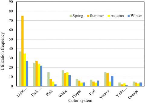
Figure 1. Utilization frequencies of different color systems in landscape images

Figure 1 shows the utilization frequencies of different color systems in landscape images. Among the spatial color systems of the landscape images in spring, summer, autumn, and winter, the light green is the most frequently utilized color system, followed in turn by dark green, yellow, white, pink, purple, and red. Currently, there are mainly two theories about color constancy. The first theory differentiates between lighting conditions and object colors through image depiction. The second theory explains the brightness and color change with the human memory process. Let (a, b) be the coordinates of any pixel in the target landscape image; ZD be the illuminance of the image; CH be the reflection property of the objects in the image; RE be the reflected light that can form an image once it is captured by the imaging device. Then, we have:

$RE(a, b)=ZD(a, b)\cdot CH(a,b)$               (1)

Formula (1) shows that the reflected light is only affected by CH and ZD. However, the impact of CH is far greater than that of ZD. If ZD can be estimated from RE and removed, then the landscape image enters the optimal state, eliminating the need for considering lighting variation. In this case, it is very likely to restore a clear landscape image.

Without any additional conditions or limitations, it is difficult to estimate the lighting and color distribution features of images accurately. If the lighting is fixed, however, the color distribution of a landscape image can form a closed and bounded convex set. This paper introduces the color constancy of landscape images to the machine learning network, and thus determines the mapping function between the color distribution features and the imaging lighting of landscape images. The landscape image lighting model needs to consider the following light factors, namely, ambient light, diffuse reflected light, specular reflected light, and light intensity attenuation.

The ambient light of landscape imaging scene may change obviously, if the weather changes from sunny to cloudy, or the other way around. The lights from all directions reach plants and buildings on different levels, and are then reflected evenly in all directions. Let RE_S be ambient light intensity; CO_S be the reflection coefficient of the object surface for ambient light. Then, the reflection intensity RE_H of ambient light can be calculated by:

$R{{E}_{H}}=R{{E}_{S}}\cdot C{{O}_{S}}$           (2)

The sun lights come from the same direction, and are reflected evenly in all directions by the plants and buildings on different landscape levels. Let M be the normal vector of plant/building surface at point O; K be the vector pointing from O to the light source, i.e., the sun; ω be the angle between M and K, i.e., the incident angle of lights; RE_G be the light source intensity; CO_M $\in$ [0, 1] be the diffuse reflection coefficient, which depends on the material attribute of plant/building, and the wavelength of the incident light. According to the law of cosines, the intensity of diffuse reflected light RE_M at O can be calculated by:

$R{{E}_{M}}=R{{E}_{G}}C{{O}_{M}}cos\omega ,\omega \in \left[ 0,\frac{\pi }{2} \right]$                (3)

Let CO_J be the specular reflection coefficient CO_J; β be the angle between the viewpoint direction U and the specular reflection direction S; m be a constant related to the smoothness of plant/building surface (the greater the value of m, the smoother the object surface). Then, the light intensity RE_J in the viewing direction of specular reflected light, which measures the level of specular reflection, can be calculated by Phong model:

$R{{E}_{J}}=R{{E}_{G}}C{{O}_{J}}co{{s}^{m}}\beta $                 (4)

If the light conditions are fixed, an object close to the light source will appear brighter than that far away from the source. Thus, the attenuation of the light intensity must be considered during the processing of landscape images. Let l be the propagation distance of light. Then, the secondary attenuation function of landscape image light intensity can be established as:

$g\left( l \right)=min\left( 1,\frac{1}{{{p}_{0}}+{{p}_{1}}l+{{p}_{2}}{{l}^{2}}} \right)$                 (5)

Formula (5) shows that the different light effects in the landscape scene can be realized by regulating the adjustment coefficients p₀, p₁ and p₂ of the computer vision system. The RGB color space can be selected to illustrate the color scene of a landscape image. Therefore, this paper decides to build a lighting model of each color component in the RGB color space. Then, the intensities of ambient light, diffuse reflected light, and specular reflected light can be respectively described as:

$R{{E}_{S}}=\left( R{{E}_{SR}},R{{E}_{SG}},R{{E}_{SB}} \right)$           (6)

$R{{E}_{M}}=\left( R{{E}_{MR}},R{{E}_{MG}},R{{E}_{MB}} \right)$                     (7)

$R{{E}_{G}}=\left( R{{E}_{GR}},R{{E}_{GG}},R{{E}_{GB}} \right)$          (8)

The coefficients of ambient light reflection CO_S, diffuse reflection CO_M, and specular reflection CO_J can be respectively calculated by:

$C{{O}_{S}}=\left( C{{O}_{SR}},C{{O}_{SG}},C{{O}_{SB}} \right)$           (9)

$C{{O}_{M}}=\left( C{{O}_{MR}},C{{O}_{MG}},C{{O}_{MB}} \right)$            (10)

$C{{O}_{J}}=\left( C{{O}_{JR}},C{{O}_{JG}},C{{O}_{JB}} \right)$                   (11)

In the RGB color space, the light intensities of the red, green, and blue channels can be respectively given by:

$\begin{align}  & R{{E}_{R}}=R{{E}_{SR}}C{{O}_{SR}}+\sum\limits_{i=1}^{m}{g\left( {{l}_{h}} \right)}R{{E}_{GR,i}}C{{O}_{MR}}\left( {{K}_{h}}\bullet M \right) \\  & +\sum\limits_{i=1}^{m}{g\left( {{l}_{h}} \right)}R{{E}_{GR,i}}C{{O}_{JR}}{{\left( {{F}_{h}}\bullet M \right)}^{m}} \\ \end{align}$                  (12)

$\begin{align}  & R{{E}_{G}}=R{{E}_{SG}}C{{O}_{SG}}+\sum\limits_{i=1}^{m}{g\left( {{l}_{h}} \right)}R{{E}_{GG,i}}C{{O}_{MG}}\left( {{K}_{h}}\bullet M \right) \\  & +\sum\limits_{i=1}^{m}{g\left( {{l}_{h}} \right)}R{{E}_{GG,i}}C{{O}_{JG}}{{\left( {{F}_{h}}\bullet M \right)}^{m}} \\ \end{align}$              (13)

$\begin{align}  & R{{E}_{B}}=R{{E}_{SB}}C{{O}_{SB}}+\sum\limits_{i=1}^{m}{g\left( {{l}_{h}} \right)}R{{E}_{GB,i}}C{{O}_{MB}}\left( {{K}_{h}}\bullet M \right) \\  & +\sum\limits_{i=1}^{m}{g\left( {{l}_{h}} \right)}R{{E}_{GB,i}}C{{O}_{JB}}{{\left( {{F}_{h}}\bullet M \right)}^{m}} \\ \end{align}$                  (14)

To simplify the adjustment of light effects, the different reflection coefficients can be decomposed as:

$\left[\begin{array}{l}C O_{S R} \\ C O_{S G} \\ C O_{S B}\end{array}\right]=C O_{S}\left[\begin{array}{c}Z D_{M R} \\ Z D_{M G} \\ Z D_{M B}\end{array}\right],\left[\begin{array}{l}C O_{M R} \\ C O_{M G} \\ C O_{M B}\end{array}\right]=C O_{M}\left[\begin{array}{c}Z D_{M R} \\ Z D_{M G} \\ Z D_{M B}\end{array}\right],\left[\begin{array}{c}C O_{J R} \\ C O_{J G} \\ C O_{J B}\end{array}\right]=C O_{J}\left[\begin{array}{c}Z D_{M R} \\ Z D_{M G} \\ Z D_{M B}\end{array}\right]$.              (15)

Formula (15) shows that, when the ambient light intensity and light source intensity of a landscape image are fixed, the surface colors of plants/buildings on different levels are jointly determined by CO_S, CO_M, and CO_J.

2.2 Landscape image enhancement

Based on color constancy, image enhancement can improve the quality of landscape images. The enhancement helps to enrich the information in the target image, improve the identification effect of the objects in the image, and promote the automatic extraction effect on the color distribution features from the image. To achieve color constant image enhancement, the premise is to ignore the landscape color features not required for image quality decline and attenuation, and to highlight the necessary features. Under this premise, the processed landscape image could be more effective than the original image in certain application scenarios.

To simplify the calculation process of color constant image enhancement, the original landscape image should be transformed to the logarithmic space, that is, the multiplication and division operations in formula (16) should be replaced with linear addition and subtraction:

$\frac{Q}{W}=\delta \left( \frac{{{l}_{2}}}{{{l}_{1}}} \right)\times \delta \left( \frac{{{l}_{3}}}{{{l}_{2}}} \right)\times \delta \left( \frac{{{l}_{4}}}{{{l}_{3}}} \right)\times ...\times \delta \left( \frac{{{l}_{m}}}{{{l}_{m}}-1} \right)$         (16)

Then, the illumination variation should be estimated by comparing the values of different pixels in the landscape image. Let [c, d] be the grayscale interval of the original landscape image g(a, b); [e, f] be the grayscale interval of h(a, b) after contrast stretching. Taking contrast stretching as a linear transform, the relationship between the original landscape image and the linearly transformed image can be characterized by:

$h\left( a,b \right)=e+\frac{f-e}{d-c}\left( g\left( a,b \right)-c \right)$                    (17)

The values of c and d can be obtained from the histograms of the original and processed landscape images, while the values of e and f can be derived from the grayscale interval of the mapping function. Since |d-c| is always smaller than |f-e|, the grayscale difference and contrast difference between pixels are increased through discretization, which does not change the number of pixels in the landscape image. The growing differences improve the quality of the landscape image, and facilitate the automatic extraction of color features. Figure 2 compares the histograms of the original and processed landscape images after color constant image enhancement.

2a.png

(a) Original image

2b.png

(b) Processed image

Figure 2. Histograms of the original and processed landscape images after color constant image enhancement

2.3 Color feature extraction from landscape images

The basic color features and dominant color system of a landscape image can be determined according to the landscape image captured in real time by the computer vision system, as well as the landscape environment information provided by field operators. Here, the relative color system bias component (CSBC) extracted from the RGB space is taken as a basic color feature of the landscape image. The greater the color system bias, the better the automatic extraction of color features. Let S_O be the CSBC of the original landscape image, and S_O be the corresponding grayscale component. Then, the relative color system bias CDC_S of the original landscape image can be calculated by:

$CD{{C}_{S}}=\frac{{{S}_{O}}-{{G}_{O}}}{{{G}_{O}}}$                (18)

The extracted relative color system bias should be normalized to further enhance the robustness of color feature extraction from landscape images under different light conditions.

Table 1 shows the composition of color clusters in landscape images. In the hue-saturation-value (HSV) color space of the landscape image colors, the H component is mostly light green, dark green, white, yellow, etc. The H value is independent of the lighting conditions of the imaging site, and related only to the colors of plants/buildings on different levels in the landscape images. Therefore, the mean value of H was selected as the color feature of landscape images. The H value can be simply calculated by:

After a landscape image completes RGB-HSV transform, the mean value of H was calculated. The greater the mean value, the smaller the CSBC. The inverse is also true.

$H\left( LI \right)=\left\{ \begin{align}  & 360-{{\cos }^{1}}\frac{\left[ \left( L{{I}_{R}}-L{{I}_{G}} \right)+\left( L{{I}_{R}}-L{{I}_{B}} \right) \right]}{2\sqrt{{{\left( L{{I}_{R}}-L{{I}_{G}} \right)}^{2}}+\left( L{{I}_{R}}-L{{I}_{B}} \right)\left( L{{I}_{G}}-L{{I}_{B}} \right)}} \\  & L{{I}_{B}}>L{{I}_{G}} \\  & {{\cos }^{-1}}\frac{\left[ \left( L{{I}_{R}}-L{{I}_{G}} \right)+\left( L{{I}_{R}}-L{{I}_{B}} \right) \right]}{2\sqrt{{{\left( L{{I}_{R}}-L{{I}_{G}} \right)}^{2}}+\left( L{{I}_{R}}-L{{I}_{B}} \right)\left( L{{I}_{R}}-L{{I}_{B}} \right)}} \\  & L{{I}_{B}}\le L{{I}_{G}} \\ \end{align} \right.$         (19)

Table 1. Composition of color clusters in landscape images

3.png

Figure 3. Analysis results on CSBC

Figure 3 presents the analysis results on CSBC. Theoretically, the color space-based CSBC analysis had a low discriminability. The color features were randomly extracted from landscape images of different seasons. For example, the green component of spring landscape images was sometimes smaller than that of autumn images. This calls for the extraction of high-level color features.

Based on machine vision and image processing, the automatic extraction of color features from landscape images aims to extract image information through computer vision system, and then classify landscape image pixels to different classes of image color features. To obtain color feature classes more accurately, this paper integrates different complementary components from multiple color spaces of the original image. Our strategy can be detailed as follows:

Step 1. Image graying is the basis of multi-color space fusion. Based on Camshift algorithm, this paper transforms the original image into a color probability distribution map, better reflection. The distribution law of the original landscape image grayscale value, using the color histograms of plants/buildings on different levels in the landscape image. The map better reflects the distribution law of grayscales in the original image. Next, other components like hue and saturation were added for further fusion.

Step 2. The background differencing algorithm was improved to quantify the feature difference between plants/buildings on different levels and the background of the landscape image in different color spaces. The improved algorithm was applied to perform differential operations on the nine color feature sub-space (CFSS) components LI_R, LI_G, LI_B, LI_H, LI_S, LI_h, LI_L, LI_a, and LI_b, which are extracted from the original landscape image in three color spaces, namely, RGB, HSV, and Lab3. In this way, 9 decomposed sub-images could be obtained

Step 3. Through the extraction and background differencing of the components from multiple color spaces and multiple CFSSs of the landscape image, the information of multiple color spaces was successfully fused based on the differential results. Let Φ₁ be the target area of the plants/buildings on different levels, which is identified through background differencing of grayscale; $\Phi_{2}, \Phi_{3} \ldots, \Phi_{q}$, q=2, 3, …, 9 be the target area identified through background differencing of the other eight components. Then, the target areas of different objects in the landscape image could be obtained through simultaneous background differencing of multiple CFSS components.

Step 4. The color results of different components were fused and denoised. To check if the landscape image contains a noise component c, it is necessary to search for K nearest neighbors similar to the image in the normalized landscape image library. Let l_cτ be the Euclidean distance between two landscape images c and τ; n be the number of image color features; φ_a be the adjustable parameter. Then, the similarity between the eigenvariables of K+1 images can be defined by:

${{O}_{c\tau }}\left( a \right)=\exp \left( -\frac{l_{c\tau }^{2}}{n{{\psi }_{a}}} \right)\text{        }\tau =1,2,...K$             (20)

The similarity in color features between landscape image c and K nearest samples can be defined as:

${{g}_{c\tau }}=1-\left| {{O}_{c\tau }}\left( a \right)-max\left( {{O}_{c\tau }}\left( b \right) \right) \right|$           (21)

There are K color feature matching scores. If the matching scores of the target landscape image are all below the preset threshold, then the image must be noisy. Therefore, the greater the K value or the preset threshold, the smaller the probability of noise presence in the landscape image. After eliminating the noise from the image, the final image color features would be exposed.

The color features of landscape images, including RE_H, RE_M, RE_J, CDC_S, hue H, CFDV, O_S and O_C, were grouped in pairs, and subject to Pearson correlation analysis. The results in Table 2 show that the RE_H of foreground plants in landscape images has a significant negative correlation with RE_J and CDC_S. To extract and classify color features from landscape images, it is often necessary to coordinate the color brightness and CSBC of plants/buildings on different levels in the images. The plants/buildings with a high hue H tend to have bright colors, and relatively large O_S and O_C. Their color features are more likely to be correctly classified.

Table 2. Correlations between color features

6.png

Figure 6. Hue values of objects on different levels

Figure 6 shows the distribution range of the hues of plants/buildings on different levels. Note that H1 and H2 stand for the hues of foreground and background objects, respectively. It can be seen that the hues of plants/buildings on different levels clustered in different areas. The H1 values of foreground plants/buildings mainly concentrated in [0°, 80°] and [230°, 260°], the intervals of red, orange, yellow, and purple color systems. The H2 values of background plants/buildings mainly concentrated in [80°, 230°], the interval of yellow and green color systems. Therefore, the foreground objects of the landscape images cover more color systems than the background objects.

7.png

Figure 7. Mean hue distribution of landscape images

According to the distribution of mean hue of landscape images (Figure 7), the landscape images after the extraction of low-level color features had smaller mean hues than those after the extraction of high-level color features. The CSBC similarity of landscape images was separately measured by angle cosine and Euclidean distance. The two metrics captured basically the same trend of hue. Of course, the CSBC obtained by Euclidean distance was larger than that obtained by angle cosine. It can be seen from Figure 7 that, the smaller the mean hue of a landscape image, the lower the extraction accuracy of its color features. This agrees with the results of manual extraction of color features. There was no obvious boundary between the hue values of low-level color extraction and those of high-level color extraction. The two sets of hues were only overlapped partially. Therefore, the color features of landscape images cannot be classified accurately, solely relying on hue. This paper introduces saturation of landscape images to the color feature analysis. Figure 8 illustrates the relationship between mean hue and mean saturation of landscape images.

8.png

Figure 8. Relationship between mean hue and mean saturation of landscape images

9.png

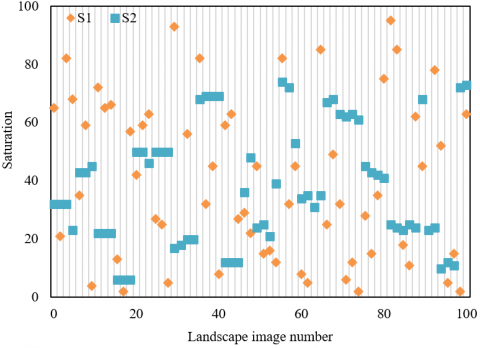
Figure 9. Saturations of objects on different levels

Figure 9 compares the statistical distributions of saturations of plants/buildings on different levels. Note that S1 and S2 stand for the saturations of foreground and background objects, respectively. It can be seen that the S1 values of foreground plants/buildings mainly concentrated in [10°, 80°], while the S2 values of background plants/buildings mainly concentrated in [0°, 90°]. There was no obvious difference between the concentration areas of the saturations for objects on different levels.

10.png

Figure 10. Values of objects on different levels

Figure 10 compares the statistical distributions of values of plants/buildings on different levels. Note that V1 and V2 stand for the values of foreground and background objects, respectively. It can be seen that the V1 values of foreground plants/buildings mainly concentrated in [60°, 95°], while the V2 values of background plants/buildings mainly concentrated in [40°, 80°]. There was an obvious difference between the concentration areas of the values for objects on different levels: the foreground plants/buildings had relatively high values; the landscape would have a better sense of depth, if the foreground and background objects have a 30% value difference.

11.png

Figure 11. Color ratios of objects on different levels

In a landscape image, the color ratio of objects refers to the color area of plants/buildings on different levels as a proportion of the total area of the landscape. Figure 11 compares the statistical distributions of color ratios of plants/buildings on different levels. It can be seen that the color ratios of foreground and background objects concentrated in [0.05, 0.35] and [0.25, 0.35], respectively. Foreground objects have a smaller color ratio than background objects.