Kazim Firildak* | Muhammed Fatih Talu
© 2021 IIETA. This article is published by IIETA and is licensed under the CC BY 4.0 license (http://creativecommons.org/licenses/by/4.0/).
OPEN ACCESS
Pneumonia, featured by inflammation of the air sacs in one or both lungs, is usually detected by examining chest X-ray images. This paper probes into the classification models that can distinguish between normal and pneumonia images. As is known, trained networks like AlexNet and GoogleNet are deep network architectures, which are widely adopted to solve many classification problems. They have been adapted to the target datasets, and employed to classify new data generated through transfer learning. However, the classical architectures are not accurate enough for the diagnosis of pneumonia. Therefore, this paper designs a capsule network with high discrimination capability, and trains the network on Kaggle’s online pneumonia dataset, which contains chest X-ray images of many adults and children. The original dataset consists of 1,583 normal images, and 4,273 pneumonia images. Then, two data augmentation approaches were applied to the dataset, and their effects on classification accuracy were compared in details. The model parameters were optimized through five different experiments. The results show that the highest classification accuracy (93.91% even on small images) was achieved by the capsule network, coupled with data augmentation by generative adversarial network (GAN), using optimized parameters. This network outperformed the classical strategies.
pneumonia, capsule network, deep convolutional generative adversarial network (DCGAN), chest X-ray, data augmentation, classification
Pneumonia, an infectious disease induced by bacteria and viruses, poses an adversely effect on human health [1]. It may cause death to children under the age of 5, the elderly, and the other individuals with a weak immune system [2]. Approximately 7% of deaths in the world are attributable to pneumonia [3, 4]. Therefore, it is critical to diagnose the disease early on. Pneumonia is generally detected by radiologists, who evaluate chest X-ray images [5]. According to the World Health Organization (WHO), only 33% of the global population can reach a radiologist capable of detecting the disease from X-ray images [6]. Hence, computer-aided decision (CmpAD) systems become increasingly important in the analysis of X-ray images.
CmpAD is the smart software that thinks and decides like a human. This software has been applied in many fields, especially in medical care [7-9]. In the medical field, CmpAD provides a strong assistance to doctors in disease diagnosis. Brinker et al. [10] compared the phenomena diagnosis by doctors without CmpAD with that by doctors aided by the software, and found that CmpAD reduced the diagnosis errors. As a result, CmpAD systems have gained popularity among doctors. Based on a hybrid deep learning (DL) model, this paper proposes a CmpAD system for pneumonia detection from X-ray images.
The application of artificial learning (AL) in medical care is mainly bottlenecked by the limited datasets and the difficulty in data collection [11]. Besides, lots of manpower, time, expert knowledge, and preprocessing technique are needed to label and classify the collected medical data. In recent years, many common medical datasets have been created and shared with researchers for the detection of specific diseases. The studies on these datasets have shown that the AL performance is proportional to the data volume. Nevertheless, the current datasets for pneumonia detection are not large enough, forcing researchers to generate synthetic data. In this paper, a deep convolutional generative adversarial network (DCGAN) is developed to augment synthetic data, and this data augmentation approach is contrasted with the classical methods.
As a subfield of AL, DL are widely applied in medical practice [11-13]. For example, chest X-ray images can be segmented by DL [14], and evaluated through DL to detect pneumonia [15]. In one of these applications, feature transfer was made from VGG16, VGG19 [16], and AlexNeT [17]; the minimum redundancy maximum relevance (mRMR) algorithm was called to select the features to be transferred; Then, the selected features were imported to a linear classifier to determine pneumonia [18]. RetinaNet [19] was also used for pneumonia detection; the detection accuracy was as high as 90.25% [20]. Recently, some scholars detected pneumonia with capsule network (CA), and grouped convolutional layers into new capsule models for disease detection [21].
This paper proposes a basic CA model [22] for pneumonia detection, which uses a GAN for data augmentation. The GAN [23] consists of a generator and a discriminator. The two modules work together to produce new images similar to training images. GAN techniques have been implemented in style transfer [24], semantic painting [25], and the solution of various medical problems [11, 26, 27]. In this paper, DCGAN [28] is designed to generate new chest X-ray images. The new images were added to the pneumonia dataset. Then, the expanded dataset was inputted to the CA classifier. To maximize the classification accuracy, the authors examined the effects of the number of convolution layers, the number of filters, and the kernel size of the CA. After that, the classification performance of the proposed method was compared with AlexNET and GoogleNET [29]. Finally, the performance of our method was evaluated by statistical metrics, and contrasted with that of existing approaches, using the pneumonia dataset.
The rest of this paper is organized as follows: Section 2 briefly introduces the dataset; Section 3 presents the classical strategy of data augmentation and the DCGAN-based data augmentation; Section 4 explains the architecture of CA; Section 5 describes the proposed hybrid architecture; Section 6 provides the experimental results of the proposed CA-DCGAN architecture, and compares the performance of our method with that of existing approaches; Section 7 draws the conclusions, and proposes ideas of future work.
The pneumonia dataset used in this study encompasses 5,856 chest X-ray images [30] on retrospective cohorts of pediatric patients aged 1-5 in Guangzhou Women and Children’s Medical Center. All of them were obtained as part of the patients’ routine clinical care.
The dataset contains 1,583 normal images, and 4,273 pneumonia images. The images (format: JPEG; color space: RGB) are of various sizes. The total size of the dataset amounts to 1GB.
To train the AL system, the chest X-ray images were labelled by two specialist doctors, and divided into a training set (5,216), a cross-validation set (16), and a test set (624). For quality control, all low-quality or unreadable scans were removed, such that all chest X-ray images are suitable for evaluation [31].
3.1 Classical approach
Data augmentation prevents the learning system from overfitting [11, 32], and thus contributes to the training and test accuracies [33]. The classical approach of data augmentation applies the following geometric and color transforms on the training image set:
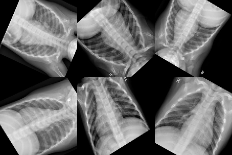
Figure 1 gives some images generated by the classical data augmentation approach.
Figure 1. Some images generated by the classical data augmentation approach
3.2 DCGAN
GANs are the first AL models that successfully produce synthetic images highly similar to real images. They have been applied in various fields, such as art, fashion, and medicine [34]. Proposed by Goodfellow et al. [23] in 2014, a typical GAN consists of two networks: a generator (G) and a discriminator (D) (Figure 2). G filters a randomly generated noisy image through specific layers to produce a new synthetic image, while D tries to distinguish between real and synthetic images (real-1; synthetic-0). Notably, the classification error of D is used to update the weights of G: the weights are updated as the inverse ratio of D’s classification success.
Figure 2. The classical GAN architecture
The G network of GAN can be trained in two steps [34, 35]:
Step 1. G takes the random noise vector z as input, and generates an image G(z);
Step 2. G generates synthetic images similar to real images to maximize D’s error [23]. The m parameter in the Eq. (1) indicates the number of input images.
$\nabla_{\theta_{g}}=\frac{1}{m} \sum_{i=1}^{m} \log \left(1-D\left(G\left(z^{i}\right)\right)\right)$ (1)
where, $\nabla_{\theta_{g}}$ is the gradient value for each weight in G. m is the number of input images.
The D network of GAN can be trained in two steps [34, 35]:
Step 1. D takes real and synthetic images as inputs;
Step 2. The gradient of each weight in D can be updated by [23]:
$\nabla_{\theta_{d}}=\frac{1}{m} \sum_{i=1}^{m}\left[\log D\left(x^{i}\right)+\log \left(1-D\left(G\left(z^{i}\right)\right)\right)\right]$ (2)
The pooling layer in D is replaced with strided convolutions, and that in G with fractional-strided convolutions.where, $\nabla_{\theta_{d}}$ is the gradient value for each weight in D. To improve the performance of classical GAN, Radford et al. [28] proposed a high-quality image generation network called DCGAN. In this network, G and D have the following unique features:
Table 1 lists all the layers in G and D of DCGAN. The G network contains 1 FC layer and 3 convolution layers. The D network contains 4 convolution layers, one flatten layer, and one FC layer. The FC layer of D has one cell.
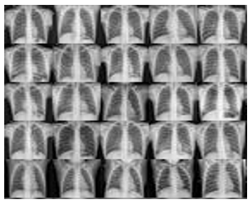
For each class of images, the DCGAN architecture was trained for 3,000 iterations, and then optimized by Adam algorithm (learning rate α=0.0002; exponential decay of the rate for moment estimates β=0.5) [36], which combines the merits of optimizers like Adagrad and RMSprop. Adam algorithm is a simple and low-cost strategy to capture momentum changes. It can be applied with a small memory, and relaxed requirements on parameters. The DCGAN is suitable to handle large and noisy datasets. Figure 3 shows some chest X-ray images generated by DCGAN.
Figure 3. Chest X-ray images generated by DCGAN
Table 1. Layers in the G and D networks of the DCGAN
|
|
Layers |
Feature Map |
Output Size |
Kernel Size |
Stride |
Activation Function |
|
G |
FC |
- |
6272 |
- |
- |
ReLU |
|
Reshape |
- |
7×7×128 |
- |
- |
- |
|
|
UpSampling2D |
- |
14×14×128 |
- |
- |
- |
|
|
Convolution2D |
128 |
14×14×128 |
3×3 |
1 |
- |
|
|
Batch Normalization |
- |
14×14×128 |
- |
- |
- |
|
|
Activation (ReLU) |
|
14×14×128 |
|
|
- |
|
|
UpSampling2D |
- |
28×28×128 |
- |
- |
- |
|
|
Convolution2D |
64 |
28×28×64 |
3×3 |
1 |
- |
|
|
Batch Normalization |
- |
28×28×64 |
- |
- |
- |
|
|
Activation (ReLU) |
|
28×28×64 |
|
|
- |
|
|
Convolution2D |
1 |
28×28×1 |
3×3 |
1 |
- |
|
|
Activation (Tanh) |
|
28×28×1 |
|
|
- |
|
|
D |
Input |
- |
28×28×1 |
- |
- |
- |
|
Convolution2D |
32 |
14×14×32 |
3×3 |
2 |
- |
|
|
Droupout (0.25) |
- |
14×14×32 |
- |
- |
- |
|
|
Convolution2D |
64 |
7×7×64 |
3×3 |
2 |
- |
|
|
Zero Padding |
- |
8×8×64 |
- |
- |
- |
|
|
Batch Normalization |
- |
8×8×64 |
- |
- |
- |
|
|
Activation (LeakyReLU(α=0.2) |
|
8×8×64 |
|
|
- |
|
|
Droupout (0.25) |
- |
8×8×64 |
- |
- |
- |
|
|
Convolution2D |
128 |
4×4×128 |
3×3 |
2 |
- |
|
|
Batch Normalization |
- |
4×4×128 |
- |
- |
- |
|
|
Activation (LeakyReLU(α=0.2) |
|
4×4×128 |
- |
- |
- |
|
|
Droupout (0.25) |
- |
4×4×128 |
- |
- |
- |
|
|
Convolution2D |
256 |
4×4×256 |
3×3 |
1 |
- |
|
|
Batch Normalization |
- |
4×4×256 |
- |
- |
- |
|
|
Activation (LeakyReLU(α=0.2) |
|
4×4×256 |
- |
- |
- |
|
|
Droupout(0.25) |
- |
4×4×256 |
- |
- |
- |
|
|
Flatten |
- |
4096 |
- |
- |
|
|
|
FC |
- |
1 |
- |
- |
Sigmoid |
The capsule network, created by Sabour et al. [22], aims to prevent the loss of features in the pooling layer of convolutional neural network (CNN). The architecture of the capsule network is shown in Figure 4.
The capsule network filters the input images with a convolution layer. At the start of training, the weights of these filters are assigned randomly in the range 0-1. The convolution process determines the number and size of filters. Through the filtering, a new image can be generated by:
$x_{i, j}^{l}=\sum_{a}^{n} \sum_{b}^{n} w_{a b} y_{(i+a)(i+b)}^{l-1}$ (3)
where, y is the input image; w is the convolution filter. Spatial derivatives (e.g., horizontal, vertical, and angular edges) and color derivatives of each input image are obtained through the convolution. The convolution results are passed to the squashing function:
$v_{j}=\frac{\left\|s_{j}\right\|^{2}}{1+\left\|s_{j}\right\|^{2}} \frac{s_{j}}{\left\|s_{j}\right\|}$ (4)
where, $v_{j}$ is the output vector of the $j \text { -th }$ capsule; $s_{j}$ is the total input. This stage is called the primary capsule.
The next stage is known as the class capsule. The prediction vectors $\hat{u}_{j \mid i}$ is calculated by multiplying each input vector of this stage with the corresponding weight ( W ). Then, the total input to a capsule $S_{j}$ is calculated as the weighted sum $\hat{u}_{j \mid i}$. The output of weighted prediction vector can be expressed as:
$s_{j}=\sum_{i} c_{i j} \hat{u}_{j \mid i}, \quad \hat{u}_{j \mid i}=w_{j \mid i} u_{i}$ (5)
where, $c_{i j}$ is a coupling coefficient determined by iterative dynamic routing:
$c_{i j}=\frac{\exp \left(b_{i j}\right)}{\sum_{k} \exp \left(b_{i k}\right)}$ (6)
where, $b_{i j}$ is the log prior probability of the $i \text { -th }$ capsule to be coupled with the $j \text { -th }$ capsule. Then, an agreed scalar value is calculated between each capsule output $v_{j} \text { in layer } j$ and the predicted $\hat{u}_{i j} \text { of the } i \text { -th }$ capsule:
$a_{i j}=v_{j} \hat{u}_{j \mid i}$ (7)
The output of the class capsule layer is predicted by the dynamic routing algorithm, whose pseudocode is given in Table 2. The number of iterations of the algorithm varies with the routing constant of the dataset.
The dynamic routing algorithm calculates the lengths of class capsule outputs, which represent the class probabilities of capsule input. Then, the margin error of the capsule network is calculated by:
$\begin{aligned}
L_{k}=& T_{k} \max \left(0, m^{+}-\left\|v_{k}\right\|\right)^{2} \\
&+\Delta\left(1-T_{k}\right) \max \left(0,\left\|v_{k}\right\|-m^{-}\right)^{2}
\end{aligned}$ (8)
where, $\mathrm{T}_{\mathrm{k}}$ is 1 if each class of the image has a single value; $\mathrm{m}^{-}=0.1, \mathrm{~m}^{+}=0.9 \text { , and } \Delta=0.5$ are constants set for the pneumonia dataset. These constants depend on the size of the dataset, and the overlap conditions.
The capsule network also has a decoder module, which receives the output from each layer of the class capsule. The loss of the capsule network is defined as the sum of margin loss and decoder loss.
Table 2. Pseudocode of the dynamic routing algorithm [22]
|
Routing Algorithm |
|
1: Routing $\left(\widehat{\boldsymbol{u}}_{j \mid i}, \boldsymbol{r}, \boldsymbol{l}\right)$ |
|
2: for all capsule i in layer l and capsule j in layer l+1: $b_{i j} \leftarrow 0$ |
|
3: for r iterations do |
|
4: for layer $\text { l: } c_{i} \leftarrow \operatorname{softmax}\left(b_{i}\right)$ |
|
5: for layer $l+1: s_{j} \leftarrow \sum_{i} c_{i j} \widehat{\boldsymbol{u}}_{j \mid i}$ |
|
6: for layer $l: v_{j}=\operatorname{squash}\left(s_{j}\right)$ |
|
7: for all capsule i in layer l and capsule j in layer l+1: $b_{i j} \leftarrow b_{i j}+\widehat{u}_{j \mid i} v_{j}$ |
|
8: return $\boldsymbol{v}_{\boldsymbol{j}}$ |
Figure 4. Process steps in a Capsule Network Architecture [22]
Figure 5. Decoder network layers
Figure 5 is the typical structure of the decoder network. The output of the network is an image reconstructed based on the capsule values. As shown in Figure 5, the decoder network consists of class CA and FC for dealing with the chest X-ray dataset. Then, the decoder network is trained by adjusting the number of Cas and the size of mini-batch. During the training, the decoder loss is added to the CA loss multiplied by 0.005. This is because the loss of the decoder layer does not change with CA loss [22]. Then, all weights of the network are updated by the Adam optimization [36].
The classification performance of medical images is positively correlated with the visual diversity of the dataset. Therefore, this paper attempts to improve the performance by adding synthetic data generation module to the classical classification architecture based on the CA.
In this section, a hybrid DL model (CA-DCGAN) is proposed for the classification of chest X-ray images. As shown in Figure 6, the CA-DCGAN integrates DCGAN with CA. The parameters of DCGAN layers in Table 1 are adopted for data generation. Unlike classical techniques of data augmentation, the GAN was selected to increase the originality of the architecture.
Facing the high-dimensional chest X-ray images, it is very complex to train the CA architectures. To reduce the training time to an acceptable length, dimensionality reduction was performed on the visual dimensions of the input. In this way, the X-ray images of different sizes (e.g., 2,090×1,858×3 and 1,553×1,044×3) were normalized as 28×28×1. The normalization speeds up the training of CA-DCGAN, and improves the efficiency of hardware utilization.
Different numbers of images were produced by DCGAN, and the training and test processes were analyzed, aiming to examine how the number of synthetic images added to the dataset influences the classification performance. Specifically, 1,800, 2,700, 3,600, 4,500, and 5,400 synthetic images were generated by DCGAN, and added to each class of the training dataset, respectively. Then, the synthetic and real data were combined and given to the CA network.
After that, the CA was trained with each of the above training datasets. The classification performance of the CA classifier on each dataset was recorded with different numbers of test images.
Figure 6. The proposed network architecture
The experiments were carried out under the framework of TensorFlow and Keras, using the programming language of Python. In the first experiment, the CA was trained on the original dataset augmented by the classical approach. Accordingly, the chest X-ray dataset was divided into a training set and a test set. The former includes 1,583 normal images, and 4,273 pneumonia images; the latter contains 234 normal images, and 390 pneumonia images. The test dataset was determined by the data provider [31].
The CA used in the experiment was trained with constants $\mathrm{m}^{-}=0.1, \mathrm{~m}^{+}=0.9, \text { and } \Delta=0.5$. The cost of the CA architecture depends on whether the image is classified correctly. If yes, the capsule output is the minimum probability with $\mathrm{m}^{+}$ parameter; otherwise, the output is the $\mathrm{m}^{-}$ parameter. Since the probability falls between 0 and 1, $\mathrm{m}^{+} \text {and } \mathrm{m}^{-}$ were set to 0.9 and 0.1, respectively. The decay $\Delta$ coefficient provides the refutation of the cost for negative classification result. The empirical value of this coefficient is 0.5. In addition, the batch sizes (32 and 64) for training were examined, and the learning rate was selected as 0.001. The CA was trained with random weights for 50 epochs. The training was carried out 5 times, and the mean results were calculated.
The experimental results were obtained using a server computer with Intel Xeon ® 2.2 GHz processor and 64GB RAM, operating on Windows Server 2012 R2. The computer programs are run on Nvidia Quadro M4000 8GB video RAM GPU card.
The performance of our algorithm and the classical method was measured by Accuracy (Acc), F-score, Precision (Pr), and Sensitivity (Se) [37]:
$A C C=\frac{T P+T N}{(T P+F N)+(F P+T N)}$ (9)
$S e=\frac{T P}{T P+F N}$ (10)
$P r=\frac{T P}{T P+F P}$ (11)
$F-\text { score }=\frac{2 x T P}{(2 x T P+F P+F N)}$ (12)
where, TP and TF are the number of correctly classified pneumonia images and normal images, respectively; FP and FN are the incorrectly classified pneumonia images and normal images, respectively. Acc, Pr, Se and F-score metrics are derived from the confusion matrix. Acc is the ratio of the number of correctly predicted images of the total number of images. Pr and Se are the precision and sensitivity values of pneumonia disease detection, respectively. The higher these values, the better the pneumonia disease is detected. The F-score is the harmonic mean Pr and Se.
A total of five experiments were carried out. In the first experiment, the dataset was expanded with the classical data augmentation approach to examine the classification performance of the CA. The shifting (1%), rotation (random in 0-2π), and cropping (1%) operations were implemented. Then, the CA training was initiated with the batch sizes of 32 and 64. Table 3 shows the classification results of the CA with different filter sizes.
Table 3. CA classification results with different filter/kernel sizes
|
Bach Size |
Kernel Size |
Filter Size |
Routing |
Acc (%) |
|
32 |
9×9 |
256 |
3 |
83.0 |
|
64 |
9×9 |
256 |
3 |
81.5 |
|
32 |
5×5 |
256 |
3 |
84.3 |
|
64 |
5×5 |
256 |
3 |
82.0 |
|
32 |
3×3 |
256 |
3 |
84.5 |
|
64 |
3×3 |
256 |
3 |
82.4 |
As shown in Table 3, the classification accuracy peaked at the filter size of 3×3. A relatively large filter size reduces the scale of the image inputted to the subsequent layers, causing a degradation of image quality. This suppresses the classification accuracy of the network.
In the second experiment, the most accurate capsule network (filter/kernel size: 3×3; batch size: 32; number of dynamic routings: 3) in the first experiment was applied with the DCGAN. The synthetic images (1,800 normal and 1,800 pneumonia) were added to the original dataset. Then, the CA was trained by the parameters of different filters and different number of convolutions. The results obtained are given in Table 4.
Table 4. Result obtained for CA with different filter sizes and increased DCGAN data
|
Layer Size |
Filter Size |
Synthetic/Real Images |
Acc (%) |
|
1 |
256 |
1800,1800 |
88.1 |
|
1 |
512 |
1800,1800 |
88.3 |
|
1 |
1024 |
1800,1800 |
88.5 |
|
2 |
128,256 |
1800,1800 |
90.0 |
As shown in Table 4, the number of filters used affected the total accuracy. The total accuracy did not change significantly, using a single convection layer and 1,024 filters. The number of convolution layers was doubled from that of the first experiment, and retraining was carried out. In this way, the highest accuracy was obtained. Hence, DCGAN data enhancement improves the classification accuracy by 5% than the classical data augmentation approach.
In the third experiment, the parameters of the convolution layer and filter numbers were fixed to analyze how the number of images synthetized by DCGAN affects the accuracy of the CA network. The relevant results are given in Table 5.
Table 5. CA different filter number and DCGAN data increase and results obtained
|
Layer Size |
Filter Size |
Synthetic/Real Images |
Acc (%) |
|
2 |
128,256 |
1800,1800 |
90 |
|
2 |
128,256 |
2700,2700 |
90.2 |
|
2 |
128,256 |
3600,3600 |
91.0 |
|
2 |
128,256 |
4500,4500 |
93.9 |
|
2 |
128,256 |
5400,5400 |
93.0 |
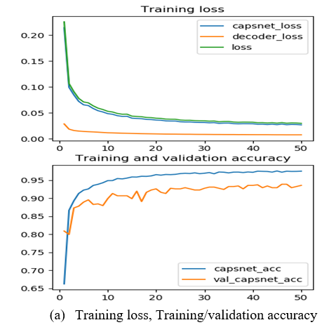
As shown in Table 5, the classification accuracy of the CA increased with the number of data. After this stage, the following numbers were all increased: the number of training data, the number of convolution layers, and the number of filters. After a certain level, it was seen that the increase in the number of layers, the number of filters and the number of sample images in the training set did not affect the test accuracy. Figure 7 presents the training loss, training accuracy, and validation accuracy of the decoder layer in the CA. It can be observed that the network achieved an accuracy of 93.91%.
In the fourth experiment, the classification performance of the proposed hybrid CA-DCGAN was compared with that of two popular classifiers, namely, AlexNet [17] and GoogleNet [29]. AlexNet has 5 convolution layers and 3 FC layers, and receives images of the size 227×227×3. The first three layers of the network are responsible to extract a general feature. The weights of these layers are transferred from the trained architecture. After being filtered through these layers, the inputs are passed through two FC layers, and classified by softmax. GoogleNet is a CNN of 22 layers. The last classification layer of this network is first removed from the general structure, and substituted by a layer trained for the classification of chest X-ray dataset. As such, the final classification layer of the network is retrained. The first layers of the network are responsible for feature extraction. For this reason, the weights of the first 10 layers are kept constant in the training stage. AlexNet, GoogleNet, and CA-DCGAN were trained for 50 epochs, at the learning rate of 0.001 and the batch size of 32. The classification accuracy and confusion matrix are recorded in Table 6 and Figure 8, respectively. In the confusion matrix, the values of 1 and 2 represent the normal class and the pneumonia class, respectively. Accuracy alone cannot fully demonstrate the classification performance. Therefore, two additional metrics were adopted, including the precision and sensitivity.
Figure 7. The proposed DCGAN-CA classification architecture results
Table 6. CA-DCGAN, AlexNet and GoogleNET results
|
Method |
Acc(%) |
Pre(%) |
Se(%) |
Fscore(%) |
|
AlexNET |
91.51 |
90.67 |
91.50 |
91.40 |
|
GoogleNET |
92.31 |
94.17 |
89.91 |
91.43 |
|
CA-DCGAN |
93.91 |
94.25 |
92.74 |
93.40 |
It can be seen that GoogleNet achieved the best FP, AlexNet realized the best FN, and our network boasted the best accuracy, sensitivity, and precision.
Figure 8. The confusion matrix obtained by the networks (CA-DCGAN, GoogleNET and AlexNET)
In the fifth experiment, our method was compared with existing methods for pneumonia classification. The classification performance is presented in Table 7. The first of the contrastive methods is CNN-based transfer learning proposed by Kermany et al. [30]. This method uses the weights transferred from the Inception3 model. After being trained for 100 epochs with a learning rate of 0.001, this method ended up with an accuracy of 92.8%. The other contrastive method is developed by Livieris et al. [38]. This method operates with the maximum likelihood selection scheme and semi-educated learning model. The proposed CA-DCGAN facilitates image classification by reducing the large images to the size of 28×28×1. As a result, our method classified low-dimensional images with a success rate of approximately 93.91%.
Table 7. Comparison with studies in the published literature on pneumonia classification
|
Study |
Model |
Acc(%) |
|
Proposed Method |
CA-DCGAN |
93.91 |
|
[38] |
Machine Learning |
83.49 |
|
[30] |
Inception V3 |
92.80 |
This paper looks for the most suitable DL architecture for pneumonia dataset. Rather than conventional deep networks, capsule network was adopted to realize the goal. Different data augmentation approaches (classical and DCGAN) were tested to improve the performance of capsule network. With the aid of DCGAN, the dataset was expanded, and the classification accuracy of the capsule network was maximized. Experimental results show that the proposed CN-DCGAN model is more accurate in classification than classic approaches (AlexNeT, GoogleNeT, Livieris’ method, and Kermany’s method). The proposed CA-DCGAN hybrid architecture can differentiate between pneumonia images and normal images with a success rate of 93.91%. In the next study, our network will be applied to limited datasets on diseases like COVID-19.
[1] Kolditz, M., Ewig, S. (2017). Community-acquired pneumonia in adults. Dtsch Aerzteblatt Online, 114: 838-48. https://doi.org/10.3238/arztebl.2017.0838
[2] Pereda, M.A., Chavez, M.A., Hooper-Miele C.C., Gilman R.H., Steinhoff, M.C., Ellington L.E., Gross, M., Price, C., Tielsch, J.M., Checkley, W. (2015). Lung ultrasound for the diagnosis of pneumonia in children: A meta-analysis. Pediatrics, 135(4): 714-722. https://doi.org/10.1542/peds.2014-2833
[3] Shen, Y., Tian Z., Lu D., Huang, J., Zhang, Z., Li, X., Li, J. (2016). Impact of pneumonia and lung cancer on mortality of women with hypertension. Scientific Reports, 6: 1-9. https://doi.org/10.1038/s41598-016-0023-2
[4] Ruuskanen, O., Lahti, E., Jennings, L.C., Murdoch D.R. (2011). Viral pneumonia. Lancet, 377: 1264-75. https://doi.org/10.1016/S0140-6736(10)61459-6
[5] World Health Organization. Pneumonia Vaccine Trial Investigators' Group & World Health Organization. (2001). Standardization of interpretation of chest radiographs for the diagnosis of pneumonia in children / World Health Organization Pneumonia Vaccine Trial Investigators' Group. World Health Organization. https://apps.who.int/iris/handle/10665/66956
[6] Aydoğdu, M., Ozyilmaz, E., Aksoy, H., Gürsel, G., Ekim, N. (2010). Mortality prediction in community-acquired pneumonia requiring mechanical ventilation; values of pneumonia and intensive care unit severity scores. Tuberkuloz ve Toraks, 58(1): 25-34.
[7] Mahomed, N., van Ginneken, B., Philipsen, R.H.H.M., Melendez, J., Moore, D.P., Moodley, H., Madhi, S.A. (2020). Computer-aided diagnosis for World Health Organization-defined chest radiograph primary-endpoint pneumonia in children. Pediatric Radiology, 50(4): 482-491. https://doi.org/10.1007/s00247-019-04593-0
[8] Tibrewala, R., Ozhinsky, E., Shah, R., Flament, I., Crossley, K., Srinivasan, R., Majumdar, S. (2020). Computer-aided detection AI reduces interreader variability in grading hip abnormalities with MRI. Journal of Magnetic Resonance Imaging, 52(4): 1163-1172. https://doi.org/10.1002/jmri.27164
[9] Carrera, E.V., Ron-Domínguez, D. (2019). A computer aided diagnosis system for skin cancer detection. International Conference on Technology Trends, Cham, pp. 553-563. https://doi.org/10.1007/978-3-030-05532-5_42
[10] Brinker, T.J., Hekler, A., Enk, A.H., Klode, J., Hauschild, A., Berking, C., Schrüfer, P. (2019). Deep learning outperformed 136 of 157 dermatologists in a head-to-head dermoscopic melanoma image classification task. European Journal of Cancer, 113: 47-54. https://doi.org/10.1016/j.ejca.2019.04.001
[11] Frid-Adar, M., Diamant, I., Klang, E., Amitai, M., Goldberger, J., Greenspan, H. (2018). GAN-based synthetic medical image augmentation for increased CNN performance in liver lesion classification. Neurocomputing, 321: 321-331. https://doi.org/10.1016/j.neucom.2018.09.013
[12] Budak, Ü., Cömert, Z., Rashid, Z.N., Şengür, A., Çıbuk, M. (2019). Computer-aided diagnosis system combining FCN and Bi-LSTM model for efficient breast cancer detection from histopathological images. Applied Soft Computing, 85: 105765. https://doi.org/10.1016/j.asoc.2019.105765
[13] Afshar, P., Plataniotis, K.N., Mohammadi, A. (2019). Capsule networks for brain tumor classification based on MRI images and coarse tumor boundaries. International Conference on Acoustics, Speech and Signal Processing (ICASSP), Brighton, pp. 1368-1372. https://doi.org/10.1109/ICASSP.2019.8683759
[14] Gómez, O., Mesejo, P., Ibáñez, O., Valsecchi, A., Cordón, O. (2019). Deep architectures for high-resolution multi-organ chest X-ray image segmentation. Neural Computing and Applications, 32: 15949-15963. https://doi.org/10.1007/s00521-019-04532-y
[15] Rajpurkar, P., Irvin, J., Zhu, K., Yang, B., Mehta, H., Duan, T., Ng, A.Y. (2017). CheXNet: Radiologist-level pneumonia detection on chest X-rays with deep learning. 3-9. http://arxiv.org/abs/1711.05225
[16] Simonyan, K., Zisserman, A. (2014). Very deep convolutional networks for large-scale image recognition. http://arxiv.org/abs/1409.1556
[17] Krizhevsky, A., Hinton, G.E. (2012). ImageNet classification with deep convolutional neural networks. International Conference on Neural Information Processing Systems, pp. 1907-1105.
[18] Toğaçar, M., Ergen, B., Cömert, Z., Özyurt, F. (2019). A deep feature learning model for pneumonia detection applying a combination of mRMR feature selection and machine learning models. IRBM, 41(4): 212-222. https://doi.org/10.1016/j.irbm.2019.10.006
[19] Lin, T.Y., Goyal, P., Girshick, R., He, K., Dollár, P. (2017). Focal loss for dense object detection. http://arxiv.org/abs/1708.02002
[20] Liu, M., Tan, Y., Chen, L. (2019). Pneumonia detection based on deep neural network Retinanet. International Conference on Image and Video Processing, and Artificial Intelligence, Shannghai, p. 44. https://doi.org/10.1117/12.2539633
[21] Mittal, A., Kumar, D., Mittal, M., Saba, T., Abunadi, I., Rehman, A., Roy, S. (2020). Detecting pneumonia using convolutions and dynamic capsule routing for chest X-ray images. Sensors, 20(4): 1068. https://doi.org/10.3390/s20041068
[22] Sabour, S., Frosst, N., Hinton, G.E. (2017). Dynamic routing between capsules. http://arxiv.org/abs/1710.09829
[23] Goodfellow, I. J., Pouget-Abadie, J., Mirza, M., Xu, B., Warde-Farley, D., Ozair, S., Courville, A., Bengio, Y. (2014). Generative adversarial networks. http://arxiv.org/abs/1406.2661
[24] Isola, P., Zhu, J.-Y., Zhou, T., Efros, A.A. (2016). Image-to-image translation with conditional adversarial networks. http://arxiv.org/abs/1611.07004
[25] Yeh, R.A., Chen, C., Lim, T.Y., Schwing, A.G., Hasegawa-Johnson, M., Do, M.N. (2016). Semantic image inpainting with deep generative models. http://arxiv.org/abs/1607.07539
[26] Bisla, D., Choromanska, A., Stein, J.A., Polsky, D., Berman, R. (2019). Towards automated melanoma detection with deep learning: Data purification and augmentation. http://arxiv.org/abs/1902.06061
[27] Xue, Y., Xu, T., Zhang, H., Long, L.R., Huang, X. (2018). SegAN: Adversarial network with multi-scale L1 loss for medical image segmentation. Neuroinformatics, 16(3-4): 383-392. https://doi.org/10.1007/s12021-018-9377-x
[28] Radford, A., Metz, L., Chintala, S. (2015). Unsupervised representation learning with deep convolutional generative adversarial networks. http://arxiv.org/abs/1511.06434
[29] Szegedy, C., Wei, L., Yangqing J., Sermanet, P., Reed, S., Anguelov, D., Rabinovich, A. (2015). Going deeper with convolutions. Conference on Computer Vision and Pattern Recognition (CVPR), Boston, pp. 1-9. https://doi.org/10.1109/CVPR.2015.7298594
[30] Kermany, D.S., Goldbaum, M., Cai, W., Valentim, C.C. S., Liang, H., Baxter, S.L., Zhang, K. (2018). Identifying medical diagnoses and treatable diseases by image-based deep learning. Cell, 172(5): 1122-1131.e9. https://doi.org/10.1016/j.cell.2018.02.010
[31] Mooney, P. (2018). Chest X-Ray Images (Pneumonia). https://www.kaggle.com/paultimothymooney/chest-xray-pneumonia, accessed on Jan. 30, 2021.
[32] Jia, S., Wang, P., Jia, P., Hu, S. (2017). Research on data augmentation for image classification based on convolution neural networks. 2017 Chinese Automation Congress (CAC), Jinan, pp. 4165-4170. https://doi.org/10.1109/CAC.2017.8243510
[33] Shashi, B. Rana, S. (2011). A review of medical image enhancement techniques for image processing. International Journal of Current Engineering and Technology, 5(2): 1282-1286. https://doi.org/10.14741/Ijcet/22774106/5.2.2015.121
[34] Langr, J., Bok, V. (2019). GANs in action. Journal of Chemical Information and Modeling Vol. 53: Shelter Island, NY / USA: Manning Publications.
[35] Goodfellow, I. (2016). NIPS 2016 tutorial: Generative adversarial networks. http://arxiv.org/abs/1701.00160
[36] Kingma, D.P., Ba, J. (2014). Adam: A method for stochastic optimization. http://arxiv.org/abs/1412.6980
[37] Powers, D.M.W. (2011). Evaluation: From precision, recall and F-measure to ROC, informedness, markedness & correlation. https://doi.org/10.9735/2229-3981
[38] Livieris, I., Kanavos, A., Tampakas, V., Pintelas, P. (2019). A weighted voting ensemble self-labeled algorithm for the detection of lung abnormalities from X-rays. Algorithms, 12(3): 64. https://doi.org/10.3390/a12030064