Liqing Xiao
© 2021 IIETA. This article is published by IIETA and is licensed under the CC BY 4.0 license (http://creativecommons.org/licenses/by/4.0/).
OPEN ACCESS
To improve the reconstruction quality of electrical resistance tomography (ERT) images, this paper designs and optimizes the finite element model for human lungs. According to the computer tomography (CT) scan image on human chest, the entire simulation domain was divided into a region of lungs, heart, and spine, and a region of adipose tissue, and the boundary curve equations of each region were derived by the improved particle swarm optimization (PSO). Based on the prior knowledge, a structural model was established for human lungs; the ERT forward problem was solved by the finite element model based on grid reconstruction, and the calculated boundary voltage of sensitivity field was taken as the theoretical value. Next, two optimization goals were set up: improving the calculation accuracy of forward problem, and easing the ill-conditionedness of the sensitivity matrix; two variables were configured: the number of layers of the finite element model in each region, and the polar diameter ratio of the finite element nodes on each layer to the finite element nodes on the boundary of each region corresponding to the same polar angle. On this basis, the finite element model was optimized by the improved PSO to adapt to human lung ERT. Simulation results show that, under the same experimental conditions, the proposed finite element model could solve the forward problem more accurately, improve the ill-conditionedness of the sensitivity matrix and the Hessian matrix, and make the sensitivity distribution more uniformly, thereby enhancing the accuracy of image reconstruction.
human lungs, electrical resistance tomography (ERT), finite element model, forward problem, sensitivity matrix, image reconstruction
As a novel technology for visualized measurement, electrical tomography (ET) is a family of process tomography (PT) techniques. Based on the different electrical features of the object in the sensitivity field, the ET techniques could be divided into electromagnetic tomography (EMT), electrical capacitance tomography (ECT), electrical impedance tomography (EIT), and electrical resistance tomography (ERT). Based on the principle of electromagnetic induction, the EMT can reconstruct the distribution state of the magnetic permeability for the medium in the sensitivity field [1-6]; Based on the principle of capacitance sensitivity, the ECT can reconstruct the distribution state of the dielectric constant for the medium in the sensitivity field [7-17]; Based on the principle of impedance sensitivity, the EIT can reconstruct the distribution state of the complex admittance for the medium in the sensitivity field [18-24]; Based on the principle of resistance sensing, the ERT can reconstruct the distribution state of the dielectric resistivity/conductivity for the medium in the sensitivity field [25-30].
As a major topic in today’s biomedical engineering, the ERT is a new-generation medical imaging technology developed after morphological and structural imaging. There are three prominent strengths of the ERT: functional imaging, noninvasiveness, and medical image monitoring. The ERT of human lungs is grounded on the principle that different tissues and organs differ in resistivity/conductivity, and every physiological and pathological condition often correspond to a certain change in the resistivity/conductivity of tissues and organs. During human lung ERT, a safe excitation current is applied to the electrode array on the body surface of the subject, creating a sensitivity field in human lungs; then, the effective boundary voltage of the field is measured by the data acquisition circuit; finally, the ERT inverse problem is solved by an image reconstruction algorithm to obtain the resistivity/conductivity distribution of tissues and organs in the sensitivity field.
Previous simulations and physical model experiments have confirmed that, for the ERT, finite element model applies to both forward and inverse problems; optimizing the finite element model helps to elevate the calculation accuracy of the forward problem, improve the ill-conditionedness of the empty field sensitivity matrix, and enhance the solution accuracy to the inverse problem [31]. Considering the peculiarity of human lung ERT, the finite element model should be optimized according to the goodness-of-fit between the model and the actual tissues and organs.
Xiao et al. [32] improved the goodness-of-fit for the region of human tissues and organs like lungs, heart, and spine, and optimized the finite element model for human lung ERT by the improved genetic algorithm (GA), with the aim to improve the calculation accuracy of the forward problem and the ill-conditionedness of the empty field sensitivity matrix. However, the inverse problem was not solved desirably due to the low goodness-of-fit for the region, as well as the assumed even distribution of tissues and organs (which varies greatly from the actual distribution). Under the same experimental conditions, the solving accuracy of the inverse problem by the image reconstruction algorithm could be improved by using a sensitivity matrix that corresponds to the close-to-actual distribution.
To solve the above defects, this paper firstly divides the finite element model for human lung ERT into a region of lungs, heart, and spine, and a region of adipose tissue, and determines the boundary curve equations of the two regions with the improved particle swarm optimization (PSO). After acquiring the theoretical boundary voltage of the sensitivity field, the authors optimized the finite element model for human lung ERT with improved PSO, in an attempt to improve the calculation accuracy of the forward problem and the ill-conditionedness of the sensitivity matrix. In this way, the authors solved the forward problem more accurately, improved the ill-conditionedness of the sensitivity matrix and the Hessian matrix, and made the sensitivity distribution more uniformly, thereby effectively enhancing the accuracy of image reconstruction.
According to the Maxwell’s equations and the Quasi-Steady-State hypothesis (QSS), the sensitivity field $\Omega$ of the ERT satisfies:
$\nabla \cdot \boldsymbol{J}=0$ (1)
where, $\nabla \cdot$ is the divergence operator; $\boldsymbol{J}$ is the current density in the sensitivity field Ω:
$\boldsymbol{J}=\sigma \cdot \boldsymbol{E}$ (2)
where, $\boldsymbol{\sigma}$ is the dielectric conductivity distribution in the sensitivity field Ω; E is the electric field strength. In the sensitivity field Ω, the potential distribution $\boldsymbol{\Phi}$ and electric field strength E basically meet the following relationship:
$\boldsymbol{E}=-\nabla \boldsymbol{\Phi}$ (3)
where, $\nabla$ is the gradient operator.
From formulas (1)-(3), the mathematical model of the ERT sensitivity field can be obtained as:
$\nabla \cdot(\sigma \nabla \boldsymbol{\Phi})=0$ (4)
Thus:
$\nabla \boldsymbol{\sigma} \cdot \nabla \boldsymbol{\Phi}+\boldsymbol{\sigma} \cdot \nabla^{2} \boldsymbol{\Phi}=0$ (5)
If medium in the sensitivity field Ω is uniform, linear, and isotropic, $\boldsymbol{\nabla} \boldsymbol{\sigma}=0$. In this case, formula (5) can be simplified to a Laplace equation:
$\nabla^{2} \boldsymbol{\Phi}=0$ (6)
where, $\nabla^{2}$ is the Laplace operator.
In the current ERT, the general practice is to apply an excitation current at the source and measure the boundary voltage of the sensitivity field. Therefore, the ERT technology satisfies the Neumann boundary condition:
$\left.\sigma \frac{\partial \boldsymbol{\Phi}}{\partial \boldsymbol{n}}\right|_{\partial \boldsymbol{\Omega}}=\boldsymbol{j}$ (7)
where, n is the outer normal direction of the boundary ∂Ω of the sensitivity field Ω; j is the current density of the boundary ∂Ω. In practice, the voltage is measured on the boundary of the sensitivity field Ω. Thus, any point $A\left(x_{0}, y_{0}\right)$ is usually selected from the sensitivity field Ω as the reference point for zero potential:
$\boldsymbol{\Phi}\left(x_{0}, y_{0}\right)=0 \quad\left(x_{0}, y_{0}\right) \in \boldsymbol{\Omega}$ (8)
The finite element model for human lung ERT was designed by dividing the entire simulation domain into a region of lungs, heart, and spine (Region 1), and a region of adipose tissue (Region 2), according to the computed tomography (CT) scan image on human chest. The finite element model was then optimized in two aspects: (1) To improve the goodness-of-fit of each region, the boundary curve equations of the two regions were determined by improved PSO; (2) To improve the calculation accuracy of the forward problem and the ill-conditionedness of the sensitivity matrix, the improved PSO was introduced to optimize the number of layers of the finite element model in each region, and the polar diameter ratio of the finite element nodes on each layer to the finite element nodes on the boundary of each region corresponding to the same polar angle.
Figure 1. The CT scan image on image on human chest
The design and optimization of the finite element model for human lung ERT were implemented in the following steps:
Step 1. According to the CT scan image on human chest (Figure 1), the entire simulation domain was divided into Region 1 and Region 2. Then, the boundary curves of the two regions were obtained by image processing. On this basis, the boundary curve equations were obtained in the form of polar coordinates:
$\bar{\rho}=\sum_{i=1}^{n} a_{i} \sin \left(b_{i} \theta+c_{i}\right)$ (9)
where, $\bar{\rho}$ is the polar diameter; θ is the polar angle; $a_{i}$, $b_{i}$, and $c_{i} \in[-10,10]$; $20 \leq n \leq 100$ is an integer (in this study, n is set to 20).
Taking $a_{i}, b_{i}$, and $c_{i}$ as variables, the fitness was calculated by:
$f(X)=\frac{1}{\sum_{i=1}^{m} \lambda_{i}\left(\bar{\rho}_{i}-\rho_{i}\right)^{2}}$ (10)
where, $X$ is a variable represented by $a_{i}, b_{i}$, and $c_{i}$$(i=1,2 \cdots n)$; m is the number of nodes on the boundary between the two regions; $\rho$ is the polar diameter of the boundary nodes; $\bar{\rho}_{i}$ and $\rho_{i}$ have the same polar angle; $\lambda_{i} \in(0,+\infty)$. The $\lambda_{i}$ value can be increased if the region is the local area of the array on body surface or region of interest (RoI), such as to further improve goodness-of-fit. In this study, $\lambda_{i}$ was set to 1.
Then, the improved PSO was introduced to determine the boundary curve equations of the two regions. By the improved PSO, the velocity V and position X of each particle can be respectively updated by:
$\left\{\begin{array}{l}\boldsymbol{V}_{i}^{k+1}=\omega \times \boldsymbol{V}_{i}^{k}+c_{1} \times \text { rand } 1 \times\left(\boldsymbol{p} \boldsymbol{b e s} \boldsymbol{t}_{i}-\boldsymbol{X}_{i}^{k}\right) \\ +c_{2} \times \text { rand } 2 \times\left(\boldsymbol{g} \boldsymbol{b} \boldsymbol{e} \boldsymbol{t}_{g}-\boldsymbol{X}_{i}^{k}\right) \\ \boldsymbol{X}_{i}^{k+1}=\boldsymbol{X}_{i}^{k}+\boldsymbol{V}_{i}^{k+1}\end{array}\right.$ (11)
$\omega=\omega_{\min }+\left(\omega_{\max }-\omega_{\min }\right) \cdot(\operatorname{maxk}-k / \operatorname{maxk})^{3}$ (12)
where, k is the number of iterations; $\operatorname{maxk}$ is the maximum number of iterations; $c_{1}$ and $c_{2}$ are learning factors; $\omega$ is the inertia weight; $\omega_{\max }$ and $\omega_{\min }$ are the maximum and minimum of the inertia weight, respectively; rand 1 and rand 2 are random numbers uniformly distributed in (0, 1).
Step 2. By the boundary curve equations of the two regions, the calculation accuracy of the forward problem was compared comprehensively; the time consumptions were measured for the calculation of the effective boundary voltage of the sensitivity field, and of the sensitivity matrix; the total number of layers was determined for the finite element model of human lung ERT [32].
Step 3. The initial finite element model was constructed model in a uniformly distributed form, according to the boundary curve equations of the two regions, and the total number of the finite element model. The triangular finite elements and nodes were numbered from inside to the outside in counterclockwise direction. When the total number of model layers and the relationship between the number of nodes on each layer and the serial number of that layer are both fixed, the finite element models with different topologies but the same numbering principle have the same the bandwidth $\gamma(\boldsymbol{K})$ of the overall stiffness matrix K, and the bandwidth of each model depends on the maximum difference between the node numbers in the same triangular finite element of the model. Therefore, the following operations were carried out after numbering finite elements and nodes to improve optimization efficiency, and avoid repeated computations of the overall stiffness matrix K:
The node number of the fixed reference potential was kept unchanged, and the node numbers in all the other triangular finite elements were taken as variables; the node numbers of the finite element model were optimized offline by the improved PSO to reduce the bandwidth $\gamma(\boldsymbol{K})$ of the overall stiffness matrix K, and thus shorten the time to calculate the effective boundary voltage of the sensitivity field. During these operations, the fitness was calculated by formula (13), and the velocity V and position X of each particle were respectively updated by formulas (11) and (12).
$f=\frac{1}{\max \left(\left|m_{i}-m_{j}\right|,\left|m_{i}-m_{k}\right|,\left|m_{k}-m_{j}\right|\right)}$ (13)
where, m is the serial number of the triangular finite element corresponding to the maximum difference between node numbers; $m_{i}, m_{j}$, and $m_{k}$ are the serial numbers of the corresponding nodes.
Step 4. According to the prior knowledge of human lungs, a structural model was set up for human lungs. Then, the finite element model based on grid reconstruction was adopted to solve the forward problem of the ERT. The resulting boundary voltage of the sensitivity field was taken as the theoretical value.
Step 5. With formula (14) as the fitness function, the finite element model was optimized to adapt to human lung ERT by improved PSO, using variables like the number of layers of the finite element model in each region, and the polar diameter ratio of the finite element nodes on each layer to the finite element nodes on the boundary of each region corresponding to the same polar angle. During the optimization, the velocity V and position X of each particle were respectively updated by formulas (11) and (12).
$F(Y)=\frac{1}{R M S \cdot \operatorname{cond}(S)}$ (14)
where, Y is a variable characterizing the number of layers of the finite element model in each region, and the polar diameter ratio of the finite element nodes on each layer to the finite element nodes on the boundary of each region corresponding to the same polar angle; RMS and S are the root mean square and sensitivity matrix corresponding to the prior knowledge model of lungs; cond is the condition number. The $R M S$ can be calculated by:
$R M S=\sqrt{\frac{1}{M} \sum_{i=1}^{M}\left(\boldsymbol{\Phi}_{F E M}-\boldsymbol{\Phi}_{\text {theory }}\right)^{2}} \times 100 \%$ (15)
where, M is the number of effective boundary voltages of the sensitivity field; $\boldsymbol{\Phi}_{F E M}$ is the effective boundary voltage of the sensitivity field calculated by the finite element model; $\boldsymbol{\Phi}_{\text {theory }}$ is the theoretical effective boundary voltage of the sensitivity field obtained in Step 4.
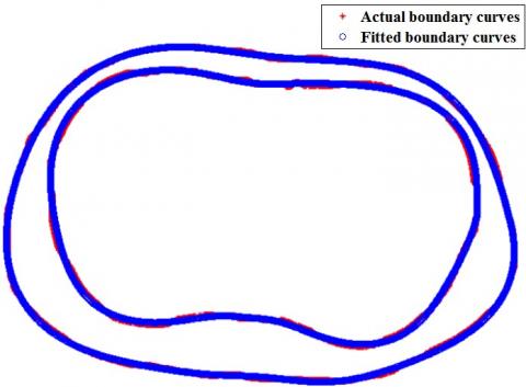
Figure 2 compares the actual boundary curves of the two regions with the curves fitted by the boundary curve equations. Obviously, the boundary curve equations obtained by the improved PSO could effectively enhance the goodness-of-fit of the two regions.
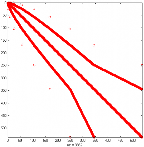
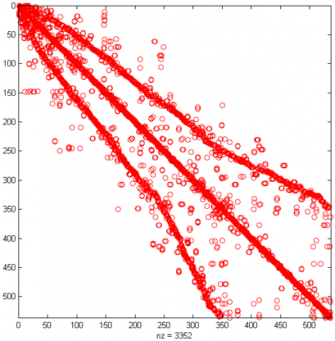
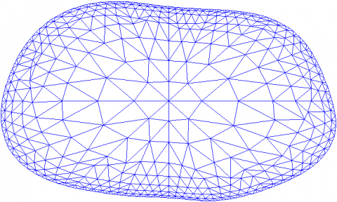
Figure 3 shows the preliminary uniformly distributed finite element model derived from the boundary curve equations of the two regions, and the total number of layers of the finite element model in each region. Figure 4 compares the bandwidth γ(K) of the overall stiffness matrix K before the node numbers are optimized by improved PSO and that after the optimization. It can be seen that, through the optimization, the bandwidth γ(K) of the overall stiffness matrix K was reduced by 34.0870% from the 575 corresponding to the serial number of commonly used nodes to 375. This greatly reduces the time to compute the effective boundary voltage of the sensitivity field, enhancing the real-time performance of the algorithm [33].
Figure 2. The comparison between actual and fitted boundary curves
Figure 3. The preliminary finite element model for human lung ERT
(a) Pre-optimization
(b) Post-optimization
Figure 4. The bandwidths γ(K) of the overall stiffness matrix K before and after optimization
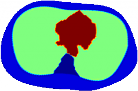
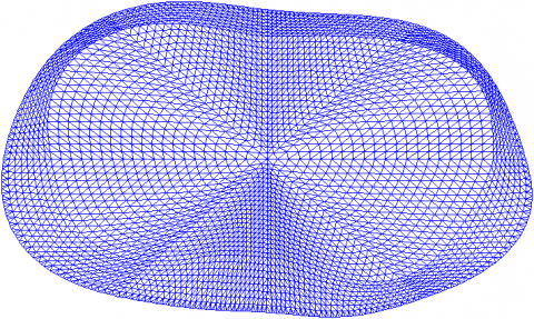
Figure 5 presents the structural model of human lungs. Figure 6 displays the finite element model, which treats the boundary voltage of the sensitivity field obtained by solving the ERT forward problem as the theoretical value. It can be seen that the model contains 3,697 nodes in 6,944 triangular finite elements.
Figure 5. The structural model of human lungs
Figure 6. The finite element model for ERT forward problem
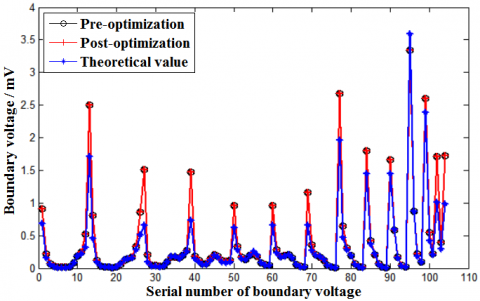
As shown in Figure 5, the RMS of the preliminary uniformly distributed finite element model was 21.1003%, and the conditional number of the corresponding sensitivity matrix was 1.2367×10⁷, according to the structural model of human lungs (Figure 5) and the theoretical boundary voltage solved by the model in Figure 6. From the boundary voltage of the sensitivity field obtained by the preliminary model (Figure 7), it can be seen that the optimization of node number does not affect the calculation accuracy of the forward problem.
Figure 7. The boundary voltage of the sensitivity field obtained by the preliminary model
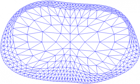
Figure 8c presents the finite element model for human lung ERT optimized by improved PSO. In Figure 8a, finite element model 1 was established by adjusting the finite element nodes to the boundary of Region 1, and using the improved PSO to optimize the number of nodes on each layer, and the polar diameter ratio of the finite element nodes to those on the boundary of Region 2 with the same polar angle. In Figure 8b, finite element model 2 was obtained by dividing the two regions according to the traditional equal interval principle. Figure 9 shows the convergence curve of the improved PSO during the optimization of finite element model 3.
(a) Finite element model 1
(b) Finite element model 2
(c) Finite element model 3
Figure 8. Three different finite element models
Figure 9. The convergence curve of the improved PSO
Figure 10 compares the boundary voltages of the sensitivity field derived by the three finite element models in Figure 8, with the boundary voltage of the sensitivity field calculated by solving the forward problem with the finite element model based on grid reconstruction as the theoretical value. The RMS values of finite element models 1-3 were .2167%, 4.1566%, and 1.4202%, respectively. Compared with models 1 and 2, the proposed model 3 lowered the RMS by 72.7759%, and 65.8327%, respectively, and effectively improved the calculation accuracy of the forward problem.
Figure 10. The comparison between the boundary voltages of the sensitivity field derived by the three finite element models
Based on the prior knowledge model of human lung (Figure 5), the condition numbers of the sensitivity matrix corresponding to finite element models 1-3 were 1.9500×10⁷, 1.3212×10⁷, and 8.4075×10⁶, respectively. Compared with models 1 and 2, the proposed model 3 reduced the condition number by 56.8846%, and 36.3647%, respectively. Hence, our model effectively improved the ill-conditionedness of the sensitivity matrix, laying the basis for high-quality image reconstruction.
In addition, the reconstruction accuracy of human lung ERT images hinges on the uniformity of the sensitivity distribution, which is usually measured by index P:
$P=\frac{\sum_{i=1} \sum_{j=2}^{k}\left|p_{i j}\right|}{k}$ (16)
where, k is the number of effective boundary voltages of the sensitivity field; $p_{i j}$ can be expressed as:
$p_{i j}=S_{i j}^{d e v} / S_{i j}^{a v g}$ (17)
where, $S_{i j}$ is the sensitivity of the electrode pair i-j; $S_{i j}^{\text {avg }}$ and $S_{i j}^{d e v}$ are the mean and standard deviation of the sensitivity matrix after the introduction of the triangular finite element area coefficient.
The smaller the P value, the better the uniformity of the sensitivity distribution, and the higher the solving accuracy of ERT inverse problem. Based on the prior knowledge model of human lung (Figure 5), the P values of finite element models 1-3 were8.1635, 8.8428, and 8.0233, respectively. Compared with models 1 and 2, the proposed model 3 reduced the P value by 1.7174%, and 9.2674%, respectively, making the sensitivity distribution more uniform.
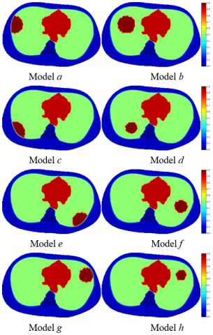
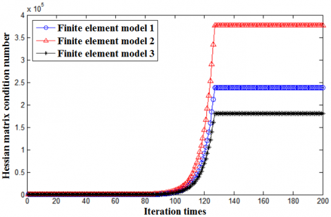
To verify the effectiveness of the proposed finite element model 3 in improving the reconstruction quality of human lung ERT images, several models were constructed for human lungs with lesions at different positions (Figure 11). Under the same experimental conditions (Intel Core Duo T8100 CPU, 3.00GB, 2.10GHz), the three finite element models and their sensitivity matrices were respectively applied to the image reconstruction by improved Newton-Raphson algorithm. Figure 12 compares the conditional numbers of the Hessian matrix corresponding to the three models during the iterative reconstruction process.
Currently, the image reconstruction quality in ERT is often evaluated by correlation coefficient and relative error:
$\rho=\frac{\sum_{i=1}^{L}\left(\hat{g}_{i}-\overline{\hat{g}}\right) \cdot\left(g_{i}-\bar{g}\right)}{\sqrt{\sum_{i=1}^{L}\left(\hat{g}_{i}-\overline{\hat{g}}\right)^{2} \sum_{i=1}^{L}\left(g_{i}-\bar{g}\right)^{2}}}$ (18)
$e=\frac{\|\boldsymbol{g}-\hat{\boldsymbol{g}}\|_{2}}{\|\boldsymbol{g}\|_{2}} \times 100 \%$ (19)
where, g is the original image; $\widehat{\boldsymbol{g}}$ is the reconstructed image; L is the number of finite elements; $\bar{g}$ and $\overline{\hat{g}}$ are the means of $\boldsymbol{g}$ and $\widehat{\boldsymbol{g}}$, respectively.
Figure 11. The models of lesions at different places of human lungs
Figure 12. The comparison between conditional numbers of Hessian matrix corresponding to the three models
The greater the correlation coefficient, the smaller the relative error, and the better the reconstruction accuracy.
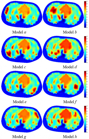
Figure 13, Table 1, and Table 2 display the reconstruction results by the three finite element models.
Table 1. The correlation coefficients of the three finite element models
|
Image |
Finite element model 1 |
Finite element model 2 |
Finite element model 3 |
|
Model a |
0.8706 |
0.8760 |
0.9359 |
|
Model b |
0.8859 |
0.8848 |
0.9357 |
|
Model c |
0.8719 |
0.8758 |
0.9347 |
|
Model d |
0.8818 |
0.8774 |
0.9344 |
|
Model e |
0.8851 |
0.8755 |
0.9296 |
|
Model f |
0.8848 |
0.8718 |
0.9346 |
|
Model g |
0.8699 |
0.8843 |
0.9332 |
|
Model h |
0.8787 |
0.8759 |
0.9322 |
Table 2. The relative errors of the three finite element models (%)
|
Image |
Finite element model 1 |
Finite element model 2 |
Finite element model 3 |
|
Model a |
30.6102 |
29.9774 |
22.8635 |
|
Model b |
28.8769 |
29.0497 |
23.0424 |
|
Model c |
30.1741 |
29.8459 |
23.1085 |
|
Model d |
29.2233 |
29.7355 |
23.0999 |
|
Model e |
28.9367 |
30.1424 |
23.7060 |
|
Model f |
29.0242 |
30.5022 |
23.0997 |
|
Model g |
30.6630 |
29.0480 |
23.1877 |
|
Model h |
29.4768 |
29.8878 |
23.2817 |
(a) Reconstruction results of finite element model 1
(b) Reconstruction results of finite element model 2
(c) Reconstruction results of finite element model 3
Figure 13. The reconstruction results of the three finite element models
As shown in Table 1, under the same experimental conditions, the mean correlation coefficients $\bar{\rho}$ of finite element models 1-3 were 0.8786, 0.8777, and 0.9338, respectively; As shown in Table 2, under the same experimental conditions, the mean relative errors of finite element models 1-3 were 29.6232%, 29.7736%, and 23.1737%, respectively. Finite element model 2 is better than finite element 1 in the calculation accuracy of forward problem, and the ill-conditionedness of the sensitivity matrix, but worse than the latter in the uniformity of sensitivity distribution, and the ill-conditionedness of Hessian matrix. Therefore, the image reconstruction quality of model 2 was not desirable.
Compared with finite element models 1 and 2, the proposed model 3 increased the correlation coefficient ${\rho}$ by an average of 6.2827%, and 6.3917%, and lowered the relative error by 21.7718%, and 22.1670%, respectively. From Figures 12-13 and Tables 1-2, our model achieved better accuracy in solving forward problem, improved the ill-conditionedness of sensitivity matrix and Hessian matrix, and made the sensitivity distribution more uniform, thereby enhancing the solving accuracy of the inverse problem.
To improve the reconstruction quality of ERT images, this paper proposes a method to design and optimize the finite element model for human lungs. Firstly, the simulation domain was split into a region of lungs, heart, and spine, and a region of adipose tissue, and the polar coordinate equations of the boundary curves were determined for each region by improved PSO, improving the goodness-of-fit of each region. On this basis, the improved PSO was further employed to optimize the number of layers of the finite element model in each region, and the polar diameter ratio of the finite element nodes on each layer to the finite element nodes on the boundary of each region corresponding to the same polar angle. In this way, the authors solved the forward problem more accurately, improved the ill-conditionedness of the sensitivity matrix and the Hessian matrix, and made the sensitivity distribution more uniformly, thereby effectively enhancing the accuracy of image reconstruction.
This work was supported by the Huainan Normal University Research and Innovation Team: Intelligent Detection Technology Research and Innovation Team (Grant No.: XJTD202009), the Key Project of Excellent Young Talents Supporting Program of Colleges and Universities in Anhui Province in 2019 (Grant No.: gxyqZD2019065).
[1] Lv, Y., He, X., Zhao, E., Deng, Y., Huang, Y., Chen, A. C. (2020). Spectral specific standardized low-resolution brain electromagnetic tomography default mode connectivity network and plasticity alterations in left vertebral artery stent patients. International Journal of Distributed Sensor Networks, 16(3): 1550147720903619. https://doi.org/10.1177/1550147720903619
[2] Wang, Q., Li, K., Zhang, R., Wang, J., Sun, Y., Li, X.Y., Duan, X.J., Wang, H.X. (2019). Sparse defects detection and 3D imaging base on electromagnetic tomography and total variation algorithm. Review of Scientific Instruments, 90(12): 124703. https://doi.org/10.1063/1.5120118
[3] Guo, C., Yang, Z., Wu, X., Tan, T., Zhao, K. (2019). Application of an adaptive multi-population parallel genetic algorithm with constraints in electromagnetic tomography with incomplete projections. Applied Sciences, 9(13): 2611. https://doi.org/10.3390/app9132611
[4] Jun, Y.H., Eom, T.H., Kim, Y.H., Chung, S.Y., Lee, I. G., Kim, J.M. (2019). Source localization of epileptiform discharges in childhood absence epilepsy using a distributed source model: a standardized, low-resolution, brain electromagnetic tomography (sLORETA) study. Neurological Sciences, 40(5): 993-1000. https://doi.org/10.1007/s10072-019-03751-4
[5] Prinsloo, S., Rosenthal, D.I., Lyle, R., Garcia, S.M., Gabel-Zepeda, S., Cannon, R., Bruera, E., Cohen, L. (2019). Exploratory study of low resolution electromagnetic tomography (LORETA) real-time Z-score feedback in the treatment of pain in patients with head and neck cancer. Brain topography, 32(2): 283-285. https://doi.org/10.1007/s10548-018-0686-z
[6] Jun, Y.H., Eom, T.H., Kim, Y.H., Chung, S.Y., Lee, I.G., Kim, J.M. (2019). Changes in background electroencephalographic activity in benign childhood epilepsy with centrotemporal spikes after oxcarbazepine treatment: a standardized low-resolution brain electromagnetic tomography (sLORETA) study. BMC neurology, 19(1): 1-8. https://doi.org/10.1186/s12883-018-1228-8
[7] Azzi, A., Bouyahiaoui, H., Berrouk, A.S., Hunt, A., Lowndes, I.S. (2020). Investigation of fluidized bed behaviour using electrical capacitance tomography. The Canadian Journal of Chemical Engineering, 98(8): 1835-1848. https://doi.org/10.1002/cjce.23748
[8] Yan, H., Wang, Y., Wang, Y.F., Zhou, Y.G. (2020). Electrical capacitance tomography image reconstruction by improved orthogonal matching pursuit algorithm. IET Science, Measurement & Technology, 14(3): 367-375. https://doi.org/10.1049/iet-smt.2019.0255
[9] Lei, J., Liu, Q.B., Wang, X.Y. (2020). Computational Imaging Method with a Learned Plug-and-Play Prior for Electrical Capacitance Tomography. Cognitive Computation, 12(1): 206-223. https://doi.org/10.1007/s12559-019-09682-8
[10] Tu, Q.Y., Wang, H.G. (2020). Investigation of the riser cross-sectional aspect ratio effect on the flow dynamics in circulating fluidized beds by electrical capacitance tomography. Transactions of the Institute of Measurement and Control, 42(4): 655-665. https://doi.org/10.1177/0142331219851913
[11] Mosorov, V., Zych, M., Hanus, R., Sankowski, D., Saoud, A. (2020). Improvement of flow velocity measurement algorithms based on correlation function and twin plane electrical capacitance tomography. Sensors, 20(1): 306. https://doi.org/10.3390/s20010306
[12] Almutairi, Z., Al-Alweet, F.M., Alghamdi, Y.A., Almisned, O.A., Alothman, O.Y. (2020). Investigating the characteristics of two-phase flow using electrical capacitance tomography (ECT) for three pipe orientations. Processes, 8(1): 51. https://doi.org/10.3390/pr8010051
[13] Maung, C.O., Kawashima, D., Darma, P.N., Takei, M. (2020). Real-time controlling particle distribution in pneumatic conveyance by electrical capacitance tomography with airflow injection system (ECT-AIS). Advanced Powder Technology, 31(6): 2530-2540. https://doi.org/10.1016/j.apt.2020.04.019
[14] Lei, J., Liu, Q.B., Wang, X.Y. (2019). Three-operator splitting scheme with the reference image regularization for electrical capacitance tomography. Neural Computing and Applications, 31(9): 5079-5096. https://doi.org/10.1007/s00521-018-04000-z
[15] Kowalska, A., Banasiak, R., Romanowski, A., Sankowski, D. (2019). 3D-printed multilayer sensor structure for electrical capacitance tomography. Sensors, 19(15): 3416. https://doi.org/10.3390/s19153416
[16] Darma, P.N., Baidillah, M.R., Sifuna, M.W., Takei, M. (2019). Improvement of image reconstruction in electrical capacitance tomography (ECT) by sectorial sensitivity matrix using a K-means clustering algorithm. Measurement Science and Technology, 30(7): 075402.
[17] Wang, R., Frias, M.A.R., Wang, H., Yang, W., Ye, J. (2018). Evaluation of electrical resistance tomography with voltage excitation compared with electrical capacitance tomography. Measurement Science and Technology, 29(12): 125401. https://doi.org/10.1088/1361-6501/aae8ff
[18] He, H., Chi, Y., Long, Y., Yuan, S., Frerichs, I., Möller, K., Fu, F., Zhao, Z. (2020). Influence of overdistension/recruitment induced by high positive end-expiratory pressure on ventilation–perfusion matching assessed by electrical impedance tomography with saline bolus. Critical Care, 24(1): 1-11. https://doi.org/10.1186/s13054-020-03301-x
[19] Garde, H. (2020). Reconstruction of piecewise constant layered conductivities in electrical impedance tomography. Communications in Partial Differential Equations, 45(9): 1118-1133. https://doi.org/10.1080/03605302.2020.1760884
[20] Secombe, C., Waldmann, A.D., Hosgood, G., Mosing, M. (2020). Evaluation of histamine‐provoked changes in airflow using electrical impedance tomography in horses. Equine veterinary journal, 52(4): 556-563. https://doi.org/10.1111/evj.13216
[21] Boyle, A., Aristovich, K., Adler, A. (2020). Beneficial techniques for spatio-temporal imaging in electrical impedance tomography. Physiological measurement, 41(6): 064003. https://doi.org/10.1088/1361-6579/ab8ccd
[22] Li, Z., Zhang, J., Liu, D., Du, J. (2019). CT image-guided electrical impedance tomography for medical imaging. IEEE transactions on medical imaging, 39(6): 1822-1832. https://doi.org/10.1109/TMI.2019.2958670
[23] Ma, G., Hao, Z., Wu, X., Wang, X. (2020). An optimal Electrical Impedance Tomography drive pattern for human-computer interaction applications. IEEE transactions on biomedical circuits and systems, 14(3): 402-411. https://doi.org/10.1109/TBCAS.2020.2967785
[24] Inany, H.S., Rettig, J.S., Smallwood, C.D., Arnold, J.H., Walsh, B.K. (2020). Distribution of ventilation measured by electrical impedance tomography in critically Ill children. Respiratory Care, 65(5): 590-595. https://doi.org/10.4187/respcare.07076
[25] Li, B., Wang, J.M., Wang, Q., Li, X.Y., Duan, X.J. (2020). A novel gas/liquid two-phase flow imaging method through electrical resistance tomography with DDELM-AE sparse dictionary. Sensor Review, 40(4): 407-420. https://doi.org/10.1108/SR-01-2019-0018
[26] Paglianti, A., Marotta, G., Montante, G. (2020). Applicability of electrical resistance tomography to the analysis of fluid distribution in haemodialysis modules. The Canadian Journal of Chemical Engineering, 98(9): 1962-1972. https://doi.org/10.1002/cjce.23826
[27] Cagáň, J., Michalcová, L. (2020). Impact damage detection in CFRP composite via electrical resistance tomography by means of statistical processing. Journal of Nondestructive Evaluation, 39(2): 1-12. https://doi.org/10.1007/s10921-020-00677-2
[28] Xiao, L.Q. (2019). Optimization of hessian matrix in modified newton-raphson algorithm for electrical resistance tomography. European Journal of Electrical Engineering, 21(5): 439-446. https://doi.org/10.18280/ejee.210506
[29] Forte, G., Albano, A., Simmons, M.J., Stitt, H.E., Brunazzi, E., Alberini, F. (2019). Assessing blending of non-newtonian fluids in static mixers by planar laser-induced fluorescence and electrical resistance tomography. Chemical Engineering & Technology, 42(8): 1602-1610. https://doi.org/10.1002/ceat.201800728
[30] Mirshekari, F., Pakzad, L. (2019). Mixing of oil in water through electrical resistance tomography and response surface methodology. Chemical Engineering & Technology, 42(5): 1101-1115. https://doi.org/10.1002/ceat.201800563
[31] Xiao, L.Q., Xue, Q., Wang, H. (2015). Finite element mesh optimisation for improvement of the sensitivity matrix in electrical resistance tomography. IET Science, Measurement & Technology, 9(7): 792-799. https://doi.org/10.1049/iet-smt.2014.0319
[32] Xiao, L.Q., Ma, Q., Wang, H. (2018). Topological structure optimization of ERT finite element model for human lung based on improved GA. In 2018 Chinese Control And Decision Conference (CCDC), pp. 5835-5839. https://doi.org/10.1109/CCDC.2018.8408151
[33] Xiao, L.Q. (2019). Finite element model and image reconstruction algorithm of electrical resistance tomography. Science Press. https://doi.org/10.7666/d.D636300