Shivali Amit Wagle* | Harikrishnan R
© 2021 IIETA. This article is published by IIETA and is licensed under the CC BY 4.0 license (http://creativecommons.org/licenses/by/4.0/).
OPEN ACCESS
Automatic identification methods for the early detection of disease in plants play a significant role in precision crop protection. Various methods have been employed in the task of plant disease recognition. This work benefits in actual identification of a plant and further detection of disease in them. In this paper, the leaf images of 9 different plants with 32 different classes of the PlantVillage database are analyzed for the process. The main contribution of this work is to classify the plant leaf disease with the proposed network-based on AlexNet and comparing with the traditional support vector machine. The convolutional neural network is used to detect the plant leaf and identify the healthy and diseased plant through this network. The mixed combination of healthy and diseased plant leaf data is used for training the convolutional neural network. Transfer learning is used for the pre-trained AlexNet network for a different amount of data for training of the network, and results are validated with a support vector machine and deep learning classifier. AlexNet performed well with an accuracy of 91.15% as compared to SVM giving 88.96% and 89.69% for radial basis function kernel and linear kernel respectively.
AlexNet, convolutional neural network, support vector machine
Plants are the backbone for all living beings as they provide food. To have good quality and quantity of the food, we need to protect the plant from the disease. The priority action is to identify the species of the plant, and followed by identifying the diseases affecting them. Having a disease in plants is quite natural, so the detection of disease in plants is very important in the field of agriculture. The plant disease severity is an important parameter and thus can be used to predict yield. Appropriate care needs to be taken to avoid the major effects on plants as they, in turn, show their effect on the product quality, quantity, or productivity. The diseases in plants cause a heavy loss in production of yield and financial loss to the farmers.
Diseases in crops are mainly classified in two types viz. airborne and soil-borne. In the air-borne type, fungal diseases are very common. The symptoms of the affected plant are seen in certain part like leaves, stem, and fruit. In soil-borne diseases, the effect is seen majorly on the roots of the plant [1]. Various types of plant disease identification techniques are used. The very basic or traditional technique is the manual inspection of the plant by naked eyes. This process was required to be carried out by experts and requires continuous monitoring over a large area of a farm [2, 3]. This process is a time-consuming and expensive one. The faster and accurate identification of the severity of the disease will help to take preventive measures and reduce the yield losses. The recognition of plant disease using images that are captured from devices like mobile phone cameras or digital cameras proves to be a significant challenge.
To overcome this situation, we are looking for a quick, reliable, automated, cost-effective, and most importantly accurate method to detect disease in the plant. A technique that automatically detects the disease symptoms in the leaves of the plant is beneficial as it reduces a lot of manual work and saves time [4]. In most cases, whenever the plant disease is detected by the farmers, they just use chemical fertilizers to prevent the crop from further growth of the disease. This could lead to a hazardous effect on the crop as well as to the person coming in contact with that crop. Sometimes using some basic things like plucking the diseased leaf and burning it or using organic fertilizers also help in solving the problem. This all depends on how much percentage of the disease has affected the leaves of the crop.
Image processing is seen to be more successfully used in disease detection mechanisms. In recent times, various machine learning algorithms for plant disease classification for certain diseases and crops have shown promising results [5]. The computer-based image processing technology applied in agricultural engineering research has become common. The Decision Trees, K-means, k nearest neighbors, Support Vector Machines (SVMs), Artificial Neural Networks (ANNs), and Machine Learning (ML) are the basic techniques used for developing the model for classification purposes. The evolution of deep learning techniques has shown significantly better results as compared to the shallow ML algorithm. The deep learning network is being used in the detection of the disease on the plant leaf that will help in faster and accurate results. The botanists are now benefitted from the advances in science and technology with computer vision approaches in the plant identification task. Several perspectives have been proposed in the literature for the classification of plants. Here the work is proposing a convolutional neural network (CNN) model for the classification of the plant. 32 classes of 9 different plants are selected from the leaf database of the PlantVillage database for this purpose. The data is classified using a support vector machine and AlexNet with transfer learning.
The organization of the paper is as follows: Related work is in section 2, proposed work using support vector machine and deep learning is discussed in section 3. Results and discussion are in section 4, followed by the Conclusion in Section 5.
There has been a lot of work done for classification purposes using various approaches. The approach of Rumpf et al. [6] for foliar sugar beet diseases using Support Vector Machine (SVM) for the feasibility of pre-symptomatic identification in the disease. The visual symptoms of plant diseases identification with SVMs were based on RGB images. The approach of Arivazhagan et al. [3] was to first convert the images from RGB to HSI image format and secondly to mask the green pixels and remove them after comparing them to the pre-calculated threshold value. Then the extraction of features is done. Textural features were extracted, and SVM was used for classification. 30 different native plants amongst the 500 plant leaves were collected from the different plant species of Tamil Nadu. The SVM classifier was also used by Neumann et al. [7] for beet leaf disease identification. The plant leaf classification is based on its different morphological features discussed by Ghaiwat and Arora [8]. The classification techniques discussed are neural network, supervised feed-forward backpropagation, unsupervised self-organizing map, Probabilistic Neural Networks, Fuzzy logic, Genetic Algorithm, SVM, Principal Component Analysis, and k-Nearest Neighbor classifier. The data was collected from village Shertha, Gujarat, India for rice plant disease viz brown spot, bacterial leaf blight, and leaf smut and was classified using SVM by Shah et al. [9]. A Genetic algorithm technique by Singh and Misra [4] for the desired segmentation and classification of the rose plant where textural features were extracted and classification was also done using SVM. The proposed algorithm by Zhang et al. [1] for cucumber leaf disease classification has used segmentation with K means, neural-network-based classification (KMSNN), SVM, plant leaf image-based classification, and textural feature classification for his work. The features need to be meticulously extracted and wisely selected from each of the diseased leaf images, and the variables in the backpropagation network and SVM need to be calibrated elaborately.
The CNN model was used to classify the apple disease with fine-grained problem in the study [10]. All the images were categorized as “healthy stage”, “early stage”, “middle stage”, or “end-stage” with the help of experts. The deep learning model of CNN were used by Lu et al. [11] and Jeon and Rhee [12] for identifying the rice disease and plant leaf recognition, respectively. The pre-trained AlexNet was used by Han et al. [13] for the classification of image scenes in remotely sensed images. If the statistical model encounters the random noise or error rather than the fundamental relationship, then there is a chance of overfitting in the deep learning models [14]. This problem can be resolved at the training stage of the model, which will enhance the intruding ability of complex conditions, wherein a slight deformation is introduced to the images at the investigational stage. A pre-trained AlexNet and VGG16 net deep learning models were used for the classification of disease was proposed by Rangarajan et al. [5]. In this case, it is seven different classes, which include six diseases and one healthy class. The classification accuracy of equal number of images for each class for tomato crop from the PlantVillage dataset is evaluated. The image data collected by Wiesner-Hanks et al. [15] from numerous stages and angles was to develop a real-time monitoring system that can focus on the phenotyping of Northern leaf blight (NLB) in maize fields using drones equipped with CNNs. Sawarkar and Kawathekar [16] focused on the classification of disease in a rose plant. The threshold techniques of native entropy and Otsu’s method were tested and the better one is used as input to the K nearest neighbor classifier. Table 1 shows the advantages and disadvantages of the models and techniques used in the field of plant disease classification. This paper presents a classification of plant and further categorize them as healthy or disease class with AlexNet and SVM.
Table 1. Advantages and disadvantages of the models and techniques in plant disease classification
|
Ref. No |
Model |
Accuracy |
Advantages |
Disadvantages |
|
[6] |
SVM is used for the classification of healthy leaves and disease class of sugarbeet |
86% |
|
|
|
[3] |
Minimum Distance Classifier and SVM for classification of ten species of plants |
87.66% |
|
|
|
[8] |
The survey of classification techniques of feed-forward backpropagation, unsupervised self-organizing map, Probabilistic Neural Networks, Fuzzy logic, Genetic Algorithm, SVM, Principal Component Analysis, and k-Nearest Neighbor classifier. |
Not applicable |
|
|
|
[4] |
Genetic algorithm with Minimum Distance Classifier and SVM for classification of plants |
93.63% and 95.71% |
|
|
|
[1] |
Cucumber disease classification using sparse representation technique. |
85.7% |
|
|
|
[10] |
VGG16 model is used for classification in the apple blackrot disease levels. |
90.4% |
|
|
|
[13] |
AlexNet for classification of rice disease classes |
90.21% |
|
|
|
[5] |
AlexNet and VGG16 in the classification of tomato plant disease. |
89.33% |
|
|
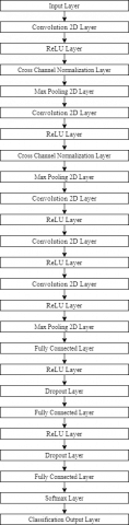
In this paper, pre-trained AlexNet with transfer learning is used for the classification of a plant leaf. Also, the performance of the network is compared with that of the traditional SVM. The proposed model for the classification of plants is as shown in Figure 1. The description of each block is explained in the further section from 3.1 to 3.5
Figure 1. Proposed model for classification of plant leaf
3.1 Healthy and diseased plant leaves dataset
The dataset of PlantVillage is taken for the classification of the plant leaf. The dataset consists of 9 different plants with healthy and disease cases. A total of 32 classes showing the variety of healthy and diseased plants from amongst the nine plants are there in the dataset. 100 images of each of the classes are selected to avoid the overfitting of data. The nine plants are apple, cherry, corn, grape, peach, pepper, potato, strawberry, and tomato. In these nine plants, one of the classes is healthy, and at least one is a diseased one.
3.2 Pre-processing of the data
For the smooth functioning of any algorithm and also to maintain uniformity in the analysis, it is necessary to follow the basic steps that are common throughout the analysis. Pre-processing is one of them. In the proposed work, SVM and AlexNet are used for classification purposes. For the AlexNet, the input requirement is that the size of the image should be $227 \times 227 \times 3 .$ The raw images chosen from the PlantVillage dataset are of size $256 \times 256 \times 3$. So, all input images are resized to the required format for AlexNet.
3.3 Generating training and testing dataset
The dataset is divided into two sets viz. training and testing dataset. In this work, an analysis of five different variations of the training dataset and the testing dataset is done. The network is trained with 10% training data, and the network is tested over the remaining data of 90%. Then the network is trained with 30% training data, and the network is tested over the remaining 70% of the data. The network is further trained with 50% training data, and the network is tested over the remaining data of 50%. Again, the network is trained with 70% of the training data, and the network is tested over the remaining data of 30%. And finally, the network is trained with 90% of training data, and the results are tested with the remaining data of 10%. These five combinations are used for training the network for the classification of the plant leaf. Table 2 shows the number of images in training data and testing data for different combinations of the total dataset, consisting of 3200 images.
Table 2. The number of images in the training and testing data set for different training data size
|
Training data size |
10% |
30% |
50% |
70% |
90% |
|
Training images |
320 |
960 |
1600 |
2240 |
2880 |
|
Testing images |
2880 |
2240 |
1600 |
960 |
320 |
3.4 Modify and apply a deep learning algorithm
The proposed idea of classification of the plant leaf is first done using the proposed AlexNet with transfer learning, and the classification is done by the state-of-the-art technique SVM with linear kernel and then using the SVM with Radial basis function (RBF) kernel. Classification of these techniques is compared with the deep learning classifier network.
3.4.1 Support Vector Machine
SVM is a supervised learning classifier. A decision plane in the SVM classifier splits between a set of objects partaking different class members. A linear classifier separates the classes into respective groups with a line. The classification of the objects is based on distinguishing the classes by drawing a separating line known as a hyperplane. SVM minimizes the high leap of the generalization error and maximizes the boundary that is created between an unravelling hyperplane and training data. SVM solves the problem caused by the error due to local minima; overfitting etc. The training data in the input space is mapped by SVM into a high-dimensional feature space. In this paper, the SVM with linear kernel and SVM with RBF kernel is used. The linear decision boundary of the feature space created is determined by generating the hyperplane distinguishing the classes. The linear SVM model scales linearly as per the size considered for the training dataset. The RBF kernel of SVM is proposed to accelerate the training time of the soft margin in the support vector machine [17]. In the SVM with RBF kernel $\left\{x_{j}^{(i)}\right\}_{j=1,2, \ldots N_{i}} \subset R^{d}$ is the set of samples from the training data in class $i$, where $N_{i}$ is the number of training samples in class $i$, with $i=1,2, L \text { and } L$ is the number of classes. The RBF kernel is
$k\left(x, x^{\prime}, \sigma\right)=\exp \left(\frac{\left\|x-x^{\prime}\right\|^{2}}{2 \sigma^{2}}\right)$ (1)
where, $x, x^{\prime} \in R^{d}-\{0\}$ is the corresponding parameter.
3.4.2 Algorithm for classification of plant leaf using Support Vector Machine with a linear kernel
The Algorithm for the classification of the plant leaf of the dataset of nine plant leaves is shown below. Step 1 to step 7 are followed for all the algorithms used in the paper. All the algorithms are implemented in MATLAB 2017B. The input size is also taken commonly in all cases.
Step 1: Read the data of healthy and diseased plant leaf
Step 2: Pre-process the data: Resize the data
Step 3: Label the data with the plant name and the healthy or disease name. e.g., Apple Healthy, Apple Black Rot, etc. for all 32 classes
Step 4: Divide the data into a training dataset and a testing dataset. The data is split into a training dataset with the variation of size having 10%, 30%, 50%, 70%, and 90% of the total data, and the remaining is used as a testing dataset in each case.
Step 5: Train the network using the training dataset for the proposed model shown in Figure 2.
Step 6: Test the network using a testing dataset using the SVM with a linear kernel.
Step 7: Calculate the performance parameters. The classification of data into the healthy or diseased plant can be done based on the performance parameters like accuracy, confusion matrix, etc.
3.4.3 Algorithm for classification of plant leaf using Support Vector Machine with Radial Basis Function kernel
The Algorithm for the classification of the plant leaf of the dataset of nine plant leaves is shown below. Step 1 to step 7 are followed in this classification task.
Step 1: Read the data of healthy and diseased plant leaf
Step 2: Pre-process the data: Resize the data
Step 3: Label the data with the plant name and the healthy or disease name. e.g., Apple Healthy, Apple Black Rot, etc. for all 32 classes
Step 4: Divide the data into a training dataset and a testing dataset. The data is split into a training dataset with the variation of size having 10%, 30%, 50%, 70%, and 90% of the total data, and the remaining is used as a testing dataset in each case.
Step 5: Train the network using the training dataset for the proposed model shown in Figure 2.
Step 6: Test the network using a testing dataset using the SVM with radial basis function kernel.
Step 7: Calculate the performance parameters. The classification of data into the healthy or diseased plant can be done based on the performance parameters like accuracy, confusion matrix, etc.
Figure 2. Network layers of the proposed model based on AlexNet
3.4.4 Deep learning methods
Deep learning models are evolved from the basic neural networks. The difference between deep learning and conventional artificial neural networks is that it has multiple numbers of hidden layers between the input and output layers. The main layer in the convolutional deep neural network model is the convolutional layer. In these models, the raw input is fed to the network to fetch certain task-specific output at the final layer of the network. Deep learning has numerous applications in the field of classification of images or recognition of voice and pattern [18, 19] in a large database. The proposed model in the study [20] a deep learning model for the “ImageNet Large Scale Visual Recognition Challenge” (ILSVRC) dataset competition where his network AlexNet was able to classify the 1000 classes. There are various convolutional neural networks (CNN) models like AlexNet, GoogLeNet, ResNet, VGG16, VGG19, DenseNet, SqueezeNet, etc. The difference in these networks is the depth in the layers and the nonlinear functions that are used in them. Otherwise, the structure is the same consisting of four important layers viz. “convolution layer”, “max-pooling layer”, “fully connected layer”, and the “output layer”.
The AlexNet is a pre-trained network that can classify 1000 classes. For the proposed work to classify the 32 classes of the dataset, transfer learning is done at the last three layers of the network. The proposed model based on AlexNet is shown in Figure 2. The results of five combinations of training testing datasets are used for all the three networks mentioned above. The classification accuracy and confusion matrix, along with the simulation time, is noted in each of the cases. In the proposed work, the classification of the leaf of nine plant varieties with 32 different classes consisting of the healthy and diseased leaf is done. In this proposed network, transfer learning was used that helps in the classification at the output layer as per the required purpose showing 32 different classes. This network consists of an input layer followed by five convolutional layers than two fully connected layers and then transfers learning layers. The requirement for the input layer is the size of the image in a specific dimension. This criterion needs to be satisfied for any CNN model. The input is convolved with the weight vectors and depending on the padding and the stride used; the layer can take up the size that is the same as before or compact or expanded. Rectified Linear Unit (ReLU) is the most frequently used as an activation function in neural networks, especially in CNNs.
$f(x)=x^{+}=\max (0, x)$ (2)
where, $\mathcal{X}$ is the input to a neuron in the network.
The probability of a vanishing gradient can be reduced by ReLU. This also introduces sparsity to the model [21]. The ReLU nonlinearity layer of the first and second convolution layers is followed by a local normalization step before doing pooling. The necessary conditions for the computational purpose and the size of it can be reduced with the help of pooling. Max pooling shows better performance and high convergence. The data is down-sampled with the help of the max-pooling layer. The chances of overfitting are reduced by this. The dropout layer offers a remarkably effective regularization and computationally cheap method to reduce overfitting problem and improve the generalization error on CNN. The first two fully connected layers are densely connected and the last fully connected layer is modified as per our requirement to predict and classify 32 different classes.
Transfer learning is the process to modify the network at the final stage for the desired output. In the transfer learning, the last three layers of the network are replaced by the fully connected layer stating the number of classified outputs that is desired, followed by the softmax activation function layer, and last the classification output layer.
3.4.5 Algorithm for classification of plant leaf using the proposed model in Figure 2 with deep learning classifier
The Algorithm for the classification of the plant leaf of the dataset of nine plant leaves is shown below. Step 1 to step 7 are followed in this classification task.
Step 1: Read the data of healthy and diseased plant leaf
Step 2: Pre-process the data: Resize the data
Step 3: Label the data with the plant name and the healthy or disease name. e.g., Apple Healthy, Apple Black Rot, etc. for all 32 classes
Step 4: Divide the data into a training dataset and a testing dataset. The data is split into a training dataset with the variation of size having 10%, 30%, 50%, 70%, and 90% of the total data, and the remaining is used as a testing dataset in each case.
Step 5: Train the network using the training dataset for the proposed model shown in Figure 2.
Step 6: Test the network using a testing dataset using the deep learning classifier.
Step 7: Calculate the performance parameters. The classification of data into the healthy or diseased plant can be done based on the performance parameters like accuracy, confusion matrix, etc.
3.5 Classify the healthy and diseased plant leaf
The classification of the healthy and diseased plant leaf is evaluated with the performance parameters. The performance parameter used for the classifier here is accuracy, confusion matrix, and the time required for computation of the classification task.
3.5.1 Accuracy of the classified output
The accuracy for the predicted output from the classifier is calculated using Eq. (3).
$\text { Accuracy }=\frac{\text { Number of correctly classified classes }}{\text { Total input classes }}$ (3)
3.5.2 Confusion matrix
The performance of the classifier is measured with the help of the confusion matrix. The confusion matrix consists of classes that are correctly classified and the classes which are misclassified. The parameters in the confusion matrix are “true positive”, “true negative”, “false positive”, and “false negative” [22]. In this work, there are 32 classes, so the confusion matrix is a multiclass one with the size of $32 \times 32$.
3.5.3 Simulation time
Time is significant in any aspect. Here the time elapsed for training and testing of the classifier for each of the case of training data of 10%, 30%, 50%, 70%, and 90% for each of the classifier i.e., SVM with linear kernel and RBF kernel, and pre-trained AlexNet with transfer learning is measured. The time is measured in seconds.
The data of 3200 images of 9 different plants with 32 classes are selected for this work. In order to make an even dataset, the data is selected with an equal number of images of each of the 32 classes. The data is classified using an SVM as well as a pre-trained AlexNet with transfer learning.
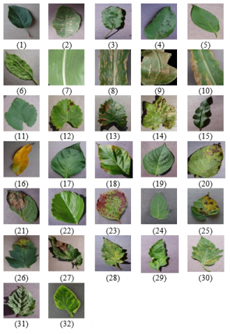
The work is done by varying the training data size by 10%, 30%, 50%, 70%, and 90% of the complete data and testing the result on the remaining data. Figure 3 shows the raw images of the plant leaf that are used for training the network. The training data in all cases is a combination of healthy and diseased plant leaves. The data is classified using three networks for various sizes of dataset size i.e., 10%, 30%, 50%, 70%, and 90% of the training data, and the results are tested on the remaining data from the dataset selected.
Figure 3. Images from the training dataset showing each of the 32 classes (1) “Apple Healthy”, (2) “Apple Cedar Rust”, (3) “Apple Black Rot”, (4) “Apple Scab”, (5) “Cherry Healthy”, (6) “Cherry Powdery Mildew”, (7) “Corn Healthy”, (8) “Corn Cercospora Leaf Spot”, (9) “Corn Common Rust”, (10) “Corn Northern Leaf Blight”, (11) “Grape Healthy”, (12) “Grape Black Rot”, (13) “Grape Black Measles”, (14) “Grape Leaf Blight”, (15) “Peach Healthy”, (16) “Peach Bacterial Spot”, (17) “Pepper Healthy”, (18) “Pepper bacterial Spot”, (19) “Potato Healthy”, (20) “Potato Early Blight”, (21) “Potato Late Blight”, (22) “Strawberry Healthy”, (23) “Strawberry Leaf Scorch”, (24) “Tomato Healthy”, (25) “Tomato Early Blight”, (26) “Tomato Bacterial Spot”, (27) “Tomato Late Blight”, (28) “Tomato Leaf Mold”, (29) “Tomato Mosaic Virus”, (30) “Tomato Septoria Leaf Spot”, (31) “Tomato Target Spot”, (32) “Tomato Yellow Leaf Curl Virus”
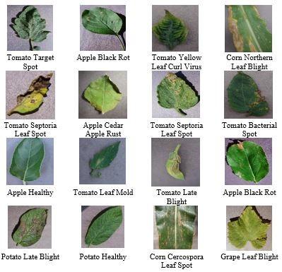
The classified images using different training data are as follows. Figure 4 shows the classified output using SVM with a linear kernel when 70% of the data is used for training and the network is tested over the remaining data. It is seen that the time required to train the network of SVM with different sizes of the dataset is not that significant as compared to the size. But the accuracy of the classified output shows significance. Figure 5 shows the classified output images using SVM with RBF kernel when 70% of the data is used for training and tested over the remaining data. The pre-trained CNN AlexNet with transfer learning is used as the other classifier in this paper. The transfer learning is used for the AlexNet here as the dataset used in this work does not have a large number of output classes to classify as compared to its capacity. The same process of training the AlexNet is implemented. Figure 6 shows the classified output images using AlexNet for 70% of the training data. The time required for training and testing the deep learning network is comparatively higher as compared to a state of art classifier. But the accuracy of the deep learning network is more as compared to the SVM classifier.
Figure 4. The classified output images using support vector machine with a linear kernel for 70% of the training data
Figure 5. The classified output images using support vector machine with RBF kernel for 70% of the training data
Table 3. The comparison of the classified output with support vector machine and AlexNet for accuracy and time elapsed in classification task
|
Parameter |
Classifier |
Training data |
||||
|
10% |
30% |
50% |
70% |
90% |
||
|
Accuracy |
SVM linear |
74.86% |
84.55% |
86.69% |
89.69% |
89.38% |
|
SVM RBF |
73.78% |
82.37% |
85.94% |
88.96% |
90.31% |
|
|
AlexNet |
73.92% |
86.43% |
86.44% |
91.15% |
90.63% |
|
|
Running Time (seconds) |
SVM linear |
2270 |
2618 |
2413 |
2361 |
2384 |
|
SVM RBF |
2471 |
2486 |
2498 |
2494 |
2234 |
|
|
AlexNet |
15671 |
21440 |
30804 |
35549 |
37653 |
|
Figure 6. The classified output images using pre-trained AlexNet with transfer learning for 70% of the training data
The comparison of the classified output with support vector machine with linear and RBF kernel and AlexNet for accuracy and elapsed time in the classification task performed by these classifiers are shown in Table 3. The accuracy for these networks is around the same when they are trained with 10% training data. The accuracy is increased from 73.78%, 82.37% and 85.37% for SVM with RBF kernel, 74.86%, 84.55% and 86.69% for SVM with linear kernel whereas the accuracy is 73.92%, 86.43% and 86.44% for AlexNet classifier. The accuracy of 91.15% is achieved for the AlexNet classifier with 70% of the training data whereas the SVM attains 88.96% and 89.69% in RBF and linear kernel. It is seen that the accuracy is increased in the case of 90% of training data for SVM but it is not the same for AlexNet. Despite using 90% training data, the accuracy for SVM is less than the 70% training data for AlexNet.
The running time required to train the network increases as the size of training data increases. At 70% of the training, data show good results as compared to time and training size for the networks. It is seen that the time required for the proposed model of deep learning network based on AlexNet is taking more time as compared to SVM classifiers. For 70% of the training data, the time required by the AlexNet model is 35549 seconds whereas the time necessary for SVM classifiers is 2361 seconds and 2494 seconds for RBF kernel and linear kernel respectively. The time invested by the deep learning algorithm is more at the cost of more accuracy as compared to SVM classifiers.
Table 4 shows the percentage accuracy of the species-wise of the plant leaf. The confusion matrix is used to identify the species wise classification of the plant leaves. The number of species for apple plant leaf is 4 having a higher accuracy of 90% by SVM. The strawberry plant with 2 types of species is showing an accuracy of 100% using AlexNet. The maximum number of species is for tomato plant with 9 types show lower accuracy in all the classifiers.
Table 4. The comparison of PlantVillage dataset of 32 classes for the classification of the plant leaf based on the confusion matrix for support vector machine and AlexNet
|
Plant name |
Number of classes |
SVM (RBF) |
SVM linear |
AlexNet
|
|
“Apple” |
4 |
90.00% |
92.50% |
93.33% |
|
“Cherry” |
2 |
95.00% |
98.33% |
95.00% |
|
“Corn” |
4 |
94.16% |
94.16% |
94.16% |
|
“Grape” |
4 |
90.83% |
95.83% |
97.50% |
|
“Peach” |
2 |
95.00% |
91.66% |
96.66% |
|
“Pepper” |
2 |
88.33% |
93.33% |
91.66% |
|
“Potato” |
3 |
88.88% |
88.88% |
90.00% |
|
“Strawberry” |
2 |
96.66% |
98.33% |
100.00% |
|
“Tomato” |
9 |
81.11% |
80.37% |
82.22% |
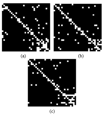
Figure 7 shows the confusion matrix for predicting the labels for all the three classifier networks. Fewer misclassifications are seen in the confusion matrix for AlexNet network as compared to SVMs. The complete analysis is done using a single CPU for the training and testing purpose.
Figure 7. Confusion matrix for classification of plant leaf with predicted classes using (a) SVM with RBF kernel, (b) SVM with linear kernel (c) AlexNet
Based on the different image classification methods, SVM being the robust model and has high prediction accuracy as compared to feed-forward backpropagation, unsupervised self-organizing map, Probabilistic Neural Networks, Fuzzy logic, Genetic Algorithm, Principal Component Analysis, and k-Nearest Neighbor classifier. Genetic Algorithm with SVM is used in early detection of disease. AlexNet is a shallower CNN model as compared to VGG16 and performs well in terms of accuracy. The performance for AlexNet model was improved with “scale pooling”, “spatial pyramid pooling”, and “side supervision” in rice disease classification. In this paper, SVM classifier has been proposed. Further a comparison of SVM with linear kernel, SVM withd RBF kernel and proposed deep network of AlexNet for the PlantVillage database for the classification of plant species and further in their respective healthy or diseased classes. It was observed that the classification accuracy (when the network is trained with 70% of the dataset) for the AlexNet is 91.15% as compared to that obtained using the SVM which is 88.96% and 89.69% for radial basis function kernel and linear kernel respectively. Moreover, the accuracy is again found to be higher for AlexNet when the network is trained with 90% of the dataset.
A total of 32 classes of nine plant species are taken into account. Strawberry with two variants of one healthy and diseased form is found to have 100% accuracy, apple with four variants of a healthy and diseased leaf is found to be 93.33% whereas the tomato plant with nine variants of a healthy and diseased class is having the lowest accuracy of 82.22% amongst all the variety of plant leaves. It is to be noted that the time required for the proposed network of AlexNet with deep learning classifier is 35549 seconds as compared to the 2361 seconds and 2494 seconds SVM classifier with linear and RBF kernel respectively.
The classification accuracy can be improved by increasing the dataset as the deep learning models can efficiently work on them. In future work, the feature extraction techniques in pre-processing of the data can be chosen that can be best suited for the deep learning model for better performance. The performance can further be improved by using a fast-computing device like GPU as the work carried out here is on a single CPU.
[1] Zhang, S., Wu, X., You, Z., Zhang, L. (2017). Leaf image based cucumber disease recognition using sparse representation classification. Computers and Electronics in Agriculture, 134: 135-141. https://doi.org/10.1016/j.compag.2017.01.014
[2] Al Bashish, D., Braik, M., Bani-Ahmad, S. (2010). A framework for detection and classification of plant leaf and stem diseases. In 2010 International Conference on Signal and Image Processing, pp. 113-118. https://doi.org/10.1109/ICSIP.2010.5697452
[3] Arivazhagan, S., Shebiah, R.N., Ananthi, S., Varthini, S.V. (2013). Detection of unhealthy region of plant leaves and classification of plant leaf diseases using texture features. Agricultural Engineering International: CIGR Journal, 15(1): 211-217.
[4] Singh, V., Misra, A.K. (2017). Detection of plant leaf diseases using image segmentation and soft computing techniques. Information Processing in Agriculture, 4(1): 41-49. https://doi.org/10.1016/j.inpa.2016.10.005
[5] Rangarajan, A.K., Purushothaman, R., Ramesh, A. (2018). Tomato crop disease classification using pre-trained deep learning algorithm. Procedia Computer Science, 133: 1040-1047. https://doi.org/10.1016/j.procs.2018.07.070
[6] Rumpf, T., Mahlein, A.K., Steiner, U., Oerke, E.C., Dehne, H.W., Plümer, L. (2010). Early detection and classification of plant diseases with support vector machines based on hyperspectral reflectance. Computers and Electronics in Agriculture, 74(1): 91-99. https://doi.org/10.1016/j.compag.2010.06.009
[7] Neumann, M., Hallau, L., Klatt, B., Kersting, K., Bauckhage, C. (2014). Erosion band features for cell phone image based plant disease classification. In 2014 22nd International Conference on Pattern Recognition, pp. 3315-3320. https://doi.org/10.1109/ICPR.2014.571
[8] Ghaiwat, S.N., Arora, P. (2014). Detection and classification of plant leaf diseases using image processing techniques: a review. International Journal of Recent Advances in Engineering & Technology, 2(3): 1-7.
[9] Shah, J.P., Prajapati, H.B., Dabhi, V.K. (2016). A survey on detection and classification of rice plant diseases. In 2016 IEEE International Conference on Current Trends in Advanced Computing (ICCTAC), pp. 1-8. https://doi.org/10.1109/ICCTAC.2016.7567333
[10] Wang, G., Sun, Y., Wang, J. (2017). Automatic image-based plant disease severity estimation using deep learning. Computational Intelligence and Neuroscience, 2017.
[11] Lu, Y., Yi, S., Zeng, N., Liu, Y., Zhang, Y. (2017). Identification of rice diseases using deep convolutional neural networks. Neurocomputing, 267: 378-384. https://doi.org/10.1016/j.neucom.2017.06.023
[12] Jeon, W.S., Rhee, S.Y. (2017). Plant leaf recognition using a convolution neural network. International Journal of Fuzzy Logic and Intelligent Systems, 17(1): 26-34. https://doi.org/10.5391/IJFIS.2017.17.1.26
[13] Han, X., Zhong, Y., Cao, L., Zhang, L. (2017). Pre-trained alexnet architecture with pyramid pooling and supervision for high spatial resolution remote sensing image scene classification. Remote Sensing, 9(8): 848. https://doi.org/10.3390/rs9080848
[14] Zhao, G., Liu, F., Oler, J.A., Meyerand, M.E., Kalin, N.H., Birn, R.M. (2018). Bayesian convolutional neural network based MRI brain extraction on nonhuman primates. Neuroimage, 175: 32-44. https://doi.org/10.1016/j.neuroimage.2018.03.065
[15] Wiesner-Hanks, T., Stewart, E.L., Kaczmar, N., DeChant, C., Wu, H., Nelson, R. J., Gore, M.A. (2018). Image set for deep learning: field images of maize annotated with disease symptoms. BMC Research Notes, 11(1): 1-3. https://doi.org/10.1186/s13104-018-3548-6
[16] Sawarkar, V., Kawathekar, S. (2018). A review: Rose plant disease detection using image processing. IOSR Journal of Computer Engineering (IOSR-JCE) https://doi.org/10.9790/0661-2004031519
[17] Kuo, B.C., Ho, H.H., Li, C.H., Hung, C.C., Taur, J.S. (2013). A kernel-based feature selection method for SVM with RBF kernel for hyperspectral image classification. IEEE Journal of Selected Topics in Applied Earth Observations and Remote Sensing, 7(1): 317-326. https://doi.org/10.1109/JSTARS.2013.2262926
[18] Ding, J., Chen, B., Liu, H., Huang, M. (2016). Convolutional neural network with data augmentation for SAR target recognition. IEEE Geoscience and Remote Sensing Letters, 13(3): 364-368. https://doi.org/10.1109/LGRS.2015.2513754
[19] Volpi, M., Tuia, D. (2016). Dense semantic labeling of subdecimeter resolution images with convolutional neural networks. IEEE Transactions on Geoscience and Remote Sensing, 55(2): 881-893. https://doi.org/10.1109/TGRS.2016.2616585
[20] Krizhevsky, A., Sutskever, I., Hinton, G.E. (2012). Imagenet classification with deep convolutional neural networks. Advances in Neural Information Processing Systems, 25: 1097-1105.
[21] Singh, U.P., Chouhan, S.S., Jain, S., Jain, S. (2019). Multilayer convolution neural network for the classification of mango leaves infected by anthracnose disease. IEEE Access, 7: 43721-43729. https://doi.org/10.1109/ACCESS.2019.2907383
[22] Barré, P., Stöver, B.C., Müller, K.F., Steinhage, V. (2017). LeafNet: A computer vision system for automatic plant species identification. Ecological Informatics, 40: 50-56. https://doi.org/10.1016/j.ecoinf.2017.05.005