Suhui Liu | Lelai Shi* | Weiyu Xu
© 2020 IIETA. This article is published by IIETA and is licensed under the CC BY 4.0 license (http://creativecommons.org/licenses/by/4.0/).
OPEN ACCESS
This work attempts to recover digital signals from a few stochastic samples in time domain. The target signal is the linear combination of one-dimensional complex sine components with R different but continuous frequencies. These frequencies control the continuous values in the domain of normalized frequency [0, 1), contrary to the previous research into compressed sensing. To recover the target signal, the problem was transformed into the completion of a low-rank structured matrix, drawing on the linear property of the Hankel matrix. Based on the completion of the structured matrix, the authors put forward a feasible-point algorithm, analyzed its convergence, and speeded up the convergence with the fast iterative shrinkage-thresholding (FIST) algorithm. The initial algorithm and the speed up strategy were proved effective through repeated numerical simulations. The research results shed new lights on the signal recovery in various fields.
signal recovery, Hankel Matrix Completion (HMC), feasible-point algorithm, fast iterative shrinkage-thresholding (FIST) algorithm
Signals contain valuable information on the attributes and actions of the emitter, and reflect the unique features of the relevant phenomena. In terms of economy, the periodic fluctuations of signals, which differ in magnitude, phase, and frequency, have attracted much attention from the academia. In many cases, however, it is difficult to extract all the information from signals, due to the limitations in sampling instruments or measuring methods. Take the extraction of frequency components for instance. Most scholars could only obtain a few discrete components from the target signal. Therefore, the signal recovery from multiple measured data is of great importance to signal processing in various fields, such as GNP cyclical fluctuations in economics [1, 2], in acceleration of medical imaging, analog-to-digital conversion, inverse scattering and in seismic imaging.
This work aims to recover a signal that linearly combines one-dimensional complex sine components with R different but continuous frequencies. To recover the entire signal, it is necessary to fully analyze the few samples of the sine components in the time domain, and measure their frequencies. This recovery task is similar to that in the signal processing of the following fields: variations in gross national product [1, 2], speeding up the capture of medical images [3], transform from analog signals to digital signals [4], and imaging of earthquake consequences [5]. The traditional strategies for the task include Prony’s approach [6], Estimation of Signal Parameters via Rotational Invariance Techniques [7], and matrix pencil [8]. In all these strategies, the sampling speed meets the Nyquist sampling theorem (NST).
As a novel technique for signal recovery, compressed sensing can recover the signal, which is sparsely or approximately sparsely distributed in a finite discrete domain, with a sample size smaller than the requirement of the NST [9] [10]. In the real-world, the signal values are usually distributed in a continuous manner. In our problem, the signal frequencies fall within the interval of [0, 1). To make compressed sensing feasible, the continuous values of the target signal could be divided into a limited number of equidistant points. Nevertheless, basis mismatch will occur if the division is not sufficiently refined [11]. In this case, the division error will be so large as to induce a huge error in signal recovery. To make matters worse, the ultrafine division of the continuous signal values will incur an unbearably high cost [12].
In recent years, more and more scholars have proposed strategies to recover continuous values based on a few discrete and unbalanced data in the time domain. For example, Candès et al. [13] minimized the total variation to pinpoint the continuous frequencies from equidistant data. Xu et al. [14] recovered the frequencies of the target signal from unbalanced data by minimizing the atomic norm. Candès et al. [13], Xu et al. [14] transformed the recovery of signal frequencies into the completion of low-rank Toeplitz matrix. Tang et al. [15] treated the signal frequency recovery of unbalanced data as a low-rank Hamiltonian Monte-Carlo problem. The above strategies can recover signals with a high robustness. But the computing efficiency is rather low in the completion of the low-rank matrices: the number of unknown factors in the optimization process is the square of the signal dimension.
Many efforts have been paid to complete the relevant matrices in an efficient manner. For instance, Candès and Recht [16] adopted interior point strategy to derive a Hessian matrix, whose scale is O(N4), in the Newtonian operation. In addition, many first-order approaches [17] were developed for matrix completion in signal recovery. Nonetheless, these approaches require an unstructured dual matrix, whose scale is O(N2). Overall, none of these approaches could efficiently recover large-dimensional signals.
To improve the efficiency of large-dimensional signal recovery, this work presents a feasible-point algorithm to complete the low-rank Hamiltonian Monte-Carlo matrix. The algorithm does not implement convex optimization of the matrix, but adopts a memory of the size O(NR), and recovers large-dimensional signal efficiently, for the number of sine components is way larger than N. Inspired by previous research [18, 19], the convergence of the algorithm to global optimal solution was analyzed in details. After that, the fast iterative shrinkage-thresholding (FIST) algorithm was referred to accelerate the convergence of our algorithm [1]. Finally, simulations confirm that the initial algorithm and the speed up strategy could recover large-dimensional signal, which linearly combines one-dimensional complex sine components with R different but continuous frequencies.
The rest of this work is arranged as follows: Chapter 2 introduces the details on the signal recovery problem; Chapter 3 presents the initial algorithm, analyzes its convergence performance, and speeds up its convergence with a self-designed algorithm; Chapter 4 verifies the feasibility of our algorithm through simulations; Chapter 5 puts forward the conclusions.
2.1 Target signal
The target signal $\begin{equation}
\tilde{x}(t), t \in \mathbb{R}
\end{equation}$ linearly combines one-dimensional complex sine components with R different but continuous frequencies [20]:
$\begin{equation}
\tilde{x}(t)=\sum_{k=1}^{R} \widetilde{d_{k}} e^{2 \pi i \widetilde{f}_{k} t}, t \geq 0
\end{equation}$ (1)
where, $\begin{equation}
\tilde{f}_{k} \in[0,1), 1 \leq k \leq R
\end{equation}$ is the frequencies; $\begin{equation}
\widetilde{d_{k}}
\end{equation}$ is the amplitudes of the complex sine components.
Traditionally, the target signal is recovered based on the data $\begin{equation}
\tilde{x}(t)
\end{equation}$, t=0, 1, …, M-1 at the integer points of the time domain. The frequencies of the target signal are obtained by linearly solving structured matrices. As mentioned before, the fully information of the target signal is not easily obtainable, owing to the constraints of instruments and environment. This is particularly true, because the target signal has large dimensions [5]. To solve the problem, the time-domain data were collected in an nonuniform manner [13, 21], which speeds up the sample collection. Let N be a sufficiently big integer, M (M<2N-1) be the number of observable data, and $\begin{equation}
\Theta \subset
\end{equation}$ {0, 1, …, 2N-2} be the index set of the observable data. Based on the collected data, the target signal can be expressed as:
$\begin{equation}
\tilde{x}(t)=[\tilde{x}(0), \tilde{x}(1), \ldots, \tilde{x}(2 N-2)]^{T} \in \mathbb{C}^{2 N-1}
\end{equation}$ (2)
2.2 Signal recovery methods
Let $\begin{equation}
\hat{x}
\end{equation}$ be the actual vector of the target signal. The recovery of this vector can be described by:
$\begin{equation}
y=\widetilde{x_{\Theta}}:=
\end{equation}$$\begin{equation}
\left\{\tilde{x}_{t} \mid t \in \Theta\right\}
\end{equation}$ (3)
The vector recovery can be solved by many methods. For example, the frequency domain [0, 1) could be meshed uniformly into grids of the size 1/(2N-1). Let F* be inverse of the 2N-1-order discrete Fourier transform matrix, $\begin{equation}
F_{\Theta}^{*}
\end{equation}$ be a row of this matrix, $\begin{equation}
c \in \mathbb{C}^{2 N-1}
\end{equation}$ be a sparse vector without any zero elements, and M be cardinality.
Assuming that the grid $\begin{equation}
\mathcal{G}
\end{equation}$ covers every frequency, the target signal could be described as $\begin{equation}
\tilde{x}=F^{*} c
\end{equation}$, and the observable data meet the condition $y=\begin{equation}
F_{\Theta}^{*} C
\end{equation}$. Then, the vector recovery becomes the recovery of sparse vector c, that is, the actual vector of the target signal. Suppose $\begin{equation}
\Theta
\end{equation}$ is a random subset extracted from {0, 1, …, 2N-2}. As long as $\begin{equation}
M \geq O(\operatorname{Klog} N)
\end{equation}$, the actual vector of the target signal can be recovered accurately by:
$\min _{c}\|c\|_{1} s . t .$$\begin{equation}
F_{\Theta}^{*} C
\end{equation}$=y (4)
Formula (4) can be solved rapidly through the strategies proposed by Beck and Teboulle [3], Yin et al. [6], Cai et al. [8], Daubechies et al. [12], and Cai et al. [22].
Assuming that the grid $\begin{equation}
\mathcal{G}
\end{equation}$ does not cover all frequencies, the actual vector of the target signal could be approximated well by solving formula (4). The deviation of the actual frequencies from the said grid could be controlled to O(1/N).
However, Tang et al. [21] argued that the above strategy leads to a large bias, even if the N value is rather big. To solve the problem, the meshing of the frequencies was replaced by considering them as continuous data in the interval [0, 1). Following this train of thoughts, two compressed sensing methods [11, 21], namely, ultra-resolution method and off-the-grid method, were designed to recover the actual vector of the target signal by:
$\min _{u, x, t} \frac{u_{0}}{2(2 N-1)}+\frac{1}{2} t, \text { s.t. }\left[\begin{array}{cc}
\mathcal{T}(u) & x \\
x^{*} & t
\end{array}\right] \geq 0$ (5)
where, $\mathcal{T}$ refers to the linear mapping to Toeplitz matrix. Suppose $\Theta$ is a random subset extracted from {0, 1, …, 2N-2}. Then, the results of formula (5) agree with the actual vector of the target signal at a high probability, which is no smaller than 1-δ. Xu et al. [14] extended the minimization of the atomic norm to the two-dimensional space.
2.3 Hankel Matrix Completion
Furthermore, Chen and Chi [17] developed a novel method to recover signals with continuous frequencies in the time domain: the task of signal recovery is transformed into the completion of Hankel matrix. The linear mapping of a vector in $\mathbb{C}^{2 N-1}$ to an N×N Hankel matrix can be described as:
$\mathcal{H}: \mathrm{x} \in \mathbb{C}^{2 N-1} \rightarrow \mathcal{H} \mathrm{x} \in \mathbb{C}^{N \times N}$,
$[\mathcal{H} \mathrm{x}]_{j k}=x_{j+k}, 0 \leq j, k \leq N-1$.
It is assumed that the R-rank Hankel matrix $\widetilde{\mathrm{H}}=\mathcal{H} \tilde{\mathrm{x}}$. Then, the rank of $\widetilde{H}$ can be factorized as:
$\left[\begin{array}{ccc}
1 & \ldots & 1 \\
e^{2 \pi l f_{1}} & \ldots & e^{2 \pi l f_{R}} \\
\vdots & \vdots & \vdots \\
e^{2 \pi l(M-1) f_{1}} & \ldots & e^{2 \pi l(M-1) f_{R}}
\end{array}\right]$ $\left[\begin{array}{lll}
\widetilde{\mathrm{d}_{1}} & & \\
& \ddots & \\
& & \widetilde{\mathrm{d}_{\mathrm{R}}}
\end{array}\right]$ $\left[\begin{array}{ccc}
1 & e^{2 \pi \imath f_{1}} \ldots & e^{2 \pi l(M-1) f_{1}} \\
\vdots & \vdots & \vdots \\
1 & e^{2 \pi l f_{R}} \ldots & e^{2 \pi l(M-1) f_{R}}
\end{array}\right]$ (6)
Next, the $\widetilde{H}$ was recovered by transforming the N×N Hankel matrix, which is converted from the vector in $\mathbb{C}^{2 N-1}$. Let $\Omega=\{(j, k) \mid j+k \in \Theta\}$ be the locations of known data in $\widetilde{H}$. Hence, the signal recovery task can be described as searching for a matrix whose rank is not greater than R, under the premise of Xjk= $\widetilde{H}$jk, (j, k)∈Ω, with X being a Hankel matrix.
Since $\mathcal{H}$ is mapped from $\mathbb{C}^{2 N-1}$ to the set of all Hankel matrices, the recovery of the actual vector of the target signal equals the recovery of $\widetilde{H}$. Inspired by Candès and Recht [16], the signal recovery task can be converted into minimizing the rank of the Hankel matrix:
$\min _{X}\|X\|_{*} s . t . X_{j k}=\widetilde{H_{j k}},(j, k) \in \Omega$ (7)
The set of every singular data $\|\mathrm{X}\|_{*}$ is called the nuclear norm. Then, formula (7) is the method designed by Chen and Chi [17]. Suppose $\Theta$ is a random subset extracted from {0, 1, …, 2N-2}. Then, the results of formula (7) are the fully recovered $\widetilde{H}$ [4]. Formula (7) is a convex optimization method. In theory, the optimization effect is very desirable. Nevertheless, the computing process of the formula is highly inefficient. The number of unknown data is as high as $O\left(N^{2}\right)$. To solve the problem, formula (7) could be transformed into a semidefinite-quadratic-linear programming problem, and be treated with the relevant software [23]. But the relevant software needs to iteratively solve a large linear system with the order $O\left(N^{2}\right) \times O\left(N^{2}\right)$. Neither could formula (7) be solved easily by algorithms that minimize the user-defined nuclear norms [24], owing to the constraint on linear equality of the Hankel matrix.
Through the above analysis, this paper directly tackles the non-convex optimization problem, which converges fast in the recovery of sparse and low-rank matrices [25, 26], and develops a feasible point algorithm for signal recovery.
3.1 Benchmark
To solve the non-convex optimization problem, the collection of smaller-than-R-order matrices with complex values and the collection of Hankel matrices with complex values that meet the observable data can be respectively expressed as:
$\mathcal{R}_{\mathbb{C}}^{R}=\left\{L \in \mathbb{C}^{N \times N} \mid \operatorname{rank}(L) \leq R\right\}$. (8)
$\mathcal{H}=\left\{\mathcal{H} x \mid x \in \mathbb{C}^{2 N-1}, x_{\Theta}=\widetilde{x_{\Theta}}\right\}$ (9)
Then, the signal recovery task and non-convex optimization can be described as:
$\min _{L \in \mathcal{R}_{\mathbb{C}, H \in \mathcal{H}}^{i n}} \frac{1}{2}\|L-H\|_{F}^{2}$ (10)
where, $\mathcal{R}_{\mathbb{C}}^{R}$ is a collection and a smooth manifold; $\mathcal{H}$ is an affine space. Formula (10) was solved by a feasible point algorithm. The objective function with the actual values of complex parameters can be expressed as: $F(L, H):=\frac{1}{2}\|L-H\|_{F}^{2}$. Complex calculus theory shows that the objective function cannot be differentiated. But this function can be differentiated into a real part $\Re$ of parameters, and an imaginary part $\Im$ of parameters. The two parts were subject to gradient flow, respectively. It is assumed that:
$Z=\left[\begin{array}{l}
\mathrm{L} \\
\mathrm{H}
\end{array}\right]=\Re+i \Im$ (11)
Then, the objective function can be rewritten as $F(\Re, \Im)$. Next, the real part was updated by $\frac{\partial F}{\partial \Re}$, while the imaginary part by $\frac{\partial F}{\partial \Im}$. That is, the initial algorithm updates Z by $\frac{\partial F}{\partial \Re}+i \frac{\partial F}{\partial \Im}$. Inspired by Fischer [27], there is:
$\frac{\partial F}{\partial \Re}+i \frac{\partial F}{\partial \Im}=2 \frac{\partial F}{\partial \bar{Z}}$ (12)
Thus:
$2 \frac{\partial F}{\partial \bar{Z}}=\left[\begin{array}{l}
2 \frac{\partial F}{\partial \bar{L}} \\
2 \frac{\partial F}{\partial \bar{H}}
\end{array}\right]=\left[\begin{array}{l}
L-H \\
H-L
\end{array}\right]$ (13)
Let $\delta_{1} \text { and } \delta_{2}$ are positive step lengths; $\mathcal{P}_{\mathcal{R}_{\mathbb{C}}^{R}} \text { and } \mathcal{P}_{\mathcal{H}}$ be the projections to $\mathcal{R}_{\mathbb{C}}^{R} \text { and } \mathcal{H}$, respectively. Then, the initial algorithm can be established as:
$\left\{\begin{array}{c}
\mathrm{L}_{t+1} \in \mathcal{P}_{\mathcal{R}_{\mathbb{C}}^{R}}\left(\mathrm{~L}_{t}-\delta_{1}\left(\mathrm{~L}_{t}-\mathrm{H}_{t}\right)\right), \\
\mathrm{H}_{t+1} \in \mathcal{P}_{\mathcal{H}}\left(\mathrm{H}_{t}-\delta_{2}\left(\mathrm{H}_{t}-\mathrm{L}_{t+1}\right)\right).
\end{array}\right.$ (14)
Then, the aim of the initial algorithm is to search for $\mathcal{P}_{\mathcal{R}_{\mathbb{C}}^{R}} \text { and } \mathcal{P}_{\mathcal{H}}$. Suppose the columns of UR and VR are the first R singular vectors of X from the left and the right, respectively; $\Sigma_{R}$ is the diagonal matrix whose elements correspond to these vectors. Drawing on Golub and Van Loan [28], $\mathcal{P}_{\mathcal{R}_{\mathbb{C}}^{R}}(\mathrm{X})$, as the optimal rank approximation to X, can be described as $\mathcal{P}_{\mathcal{R}_{\mathbb{C}}^{R}}(\mathrm{X})=\mathrm{U}_{R} \Sigma_{R} \mathrm{~V}_{R}^{*}$. Then, the following lemma was proposed to describe $\mathcal{P}_{\mathcal{H}}$ in its closed form Lemma 1:
$\mathcal{P}_{\mathcal{H}}(\mathrm{X})=\mathcal{H} \mathrm{z}$,
where $z_{j}=\left\{\begin{array}{cc}
\tilde{x}_{j}, & \text { if } j \in \Theta \\
\operatorname{mean}\left\{X_{k l} \mid k+l=j\right\}, & \text { otherwise }
\end{array}\right..$ (15)
Proof. $\mathcal{P}_{\mathcal{H}}(\mathrm{X})$ is the results of the LS (least squares) problem:
$\mathcal{P}_{\mathcal{H}}(Z)=\operatorname{argmin}_{Z}\left\{\|Z-X\|_{F}^{2}: W \in \mathcal{H}\right\}$
$=\mathcal{H} \cdot \operatorname{argmin}_{z}\left\{\|\mathcal{H} z-X\|_{F}^{2}: z_{\Theta}=\tilde{x}_{\Theta}\right\}$
$=\mathcal{H} \cdot \operatorname{argmin}_{z}\left\{\sum_{j=0}^{2 N-2}\left[\sum_{k+l=j}\left(z_{j}-X_{k l}\right)^{2}: z_{\Theta}=\tilde{x}_{\Theta}\right]\right\}$ (16)
The results in the last row are clearly the zj in formula (15). Q.E.D. During the iteration of our feasible-point algorithm, Lt and Ht separately fall into the sets of feasible values $\mathcal{R}_{\mathbb{C}}^{R} \text { and } \mathcal{H}$, which minimizes the computing load and memory occupation, provided that R is less than N. Whereas $\mathrm{L}_{t} \in \mathcal{R}_{\mathbb{C}}^{R}$, the relevant results only occupy a memory of O(NR). Moreover, the parametric representation of Ht only occupies a space of O(N). In addition, the initial algorithm only has to calculate the first R singular values and the relevant vectors during the projection computation. The computation can be completed without calling anything other than the matrix vector product (MVP) of $L_{t}-\delta_{1}\left(L_{t}-H_{t}\right)$. The MVP of Lt, which is an R-rank factorized value, can be computed in only O(NR) steps. Through fast Fourier transform [28], the MVP of Ht can be computed in only O(NlogN) steps. The second step of the initial algorithm only need to average Lt+1 along anti-diagonals [29-34].
3.2 Convergence analysis
Based on the data of Attouch et al. [18], the convergence of the initial algorithm was analyzed. Let us denote proper and lower semi-continuous (PLSC) functions as$\theta: \mathbb{R}^{n} \mapsto \mathbb{R} \cup\{+\infty\} \text { and } \omega: \mathbb{R}^{m} \mapsto \mathbb{R} \cup\{+\infty\}$, and C1 function as $\phi: \mathbb{R}^{n} \times \mathbb{R}^{m} \mapsto \mathbb{R}$. In general, the non-convex optimization can be described as:
$\min _{x, y} \psi(x, y):=\phi(x, y)+\theta(x)+\omega(y)$ (17)
Drawing on Attouch et al. [18], formula (17) was solved through proximal alternating minimization:
$\left\{\begin{array}{c}
\mathrm{x}_{k+1} \in \operatorname{argmin}_{\mathrm{x} \in \mathbb{B}^{n}} \psi\left(\mathrm{x}, \mathrm{y}_{k}\right)+\frac{1}{2 \lambda_{k}}\left\|\mathrm{x}-\mathrm{x}_{k}\right\|_{2}^{2}, \\
\mathrm{y}_{k+1} \in \operatorname{argmin}_{\mathrm{y} \in \mathbb{R}^{m}} \psi\left(\mathrm{x}_{k+1}, \mathrm{y}\right)+\frac{1}{2 \mu_{k}}\left\|\mathrm{y}-\mathrm{y}_{k}\right\|_{2}^{2}.
\end{array}\right.$ (18)
Suppose function $\psi$ meets the Kurdyka-Lojasiewicz condition, and that $\nabla \phi$ is Lipschitz on bounded sets. Then, the convergence of formula (17) could be proved by the method specified by Attouch et al. [18]. Since it is difficult to verify, the Kurdyka-Lojasiewicz condition could be guaranteed by the semi-algebraic SA property. A PLSC function has SA property, as long as its graph forms an SA set. The condition for a subset $S \subset \mathbb{R}^{d}$ to be a real SA set was defined as follows: there is a limited number of real polynomial functions $g_{i j}, h_{i j}: \mathbb{R}^{d} \mapsto \mathbb{R}$ so that:
S=$\bigcup_{j=1}^{p} \bigcap_{i=1}^{q}$$\left\{\mathrm{u} \in \mathbb{R}^{d} \mid g_{i j}(\mathrm{u})=0, h_{i j}(\mathrm{u})<0\right\}$ (19)
Then, the sets $C \in \mathbb{R}^{n} \text { and } D \in \mathbb{R}^{m}$ were respectively indicated by functions $\theta=\delta_{C} \text { and } \omega=\delta_{D}$. Then, set C could be indicated by $\delta_{C}(\mathrm{x})=\left\{\begin{array}{cl}
0, & \text { if } \mathrm{x} \in C, \\
+\infty, & \text { if } \mathrm{x} \notin C .
\end{array}\right.$ Under the condition that $\phi(x, y)=\frac{1}{2}\|x-y\|_{2}^{2}$, the non-convex optimization can be converted into an alternating projection:
$\left\{\begin{array}{c}
\mathrm{x}_{k+1} \in \mathcal{P}_{C}\left(\mathrm{x}_{k}-\frac{1}{1+\delta_{k}}\left(\mathrm{x}_{k}-\mathrm{y}_{k}\right)\right), \\
\mathrm{y}_{k+1} \in \mathcal{P}_{D}\left(\mathrm{y}_{k}-\frac{1}{1+\mu_{k}}\left(\mathrm{y}_{k}-\mathrm{x}_{k+1}\right)\right).
\end{array}\right.$ (20)
According to Bolte et al. [7] and Attouch et al. [18], the convergence of formula (18) can be described by the following theorem.
Theorem 1. It is assumed that $C \subset \mathbb{R}^{n} \text { and } D \subset \mathbb{R}^{m}$ have SA property. Then, the alternating projection can produce (xk, yk), where 0<a<δk, and μk<b for all k:
Case 1: $\left\|\left(\mathrm{x}_{k}, \mathrm{y}_{k}\right)\right\|_{2} \rightarrow \infty \text { as } k \rightarrow \infty$, or (xk, yk) converges to a critical point of $\psi$;
Case 2: If (x0, y0) is feasible and sufficiently close to a global minimizer of $\psi$, (x0, y0) converges to that minimizer.
Further, the above theorem was introduced to the initial algorithm to test its convergence performance. Although the initial algorithm takes the same shape as alternating projection, the above theorem targets real numbers, while the initial algorithm handles the matrix space with complex values. Fortunately, any matrix with complex values could be converted into a matrix with real number by merging the real part with imaginary part. As stated before, the initial algorithm was constructed based on the gradient of the two parts. Because the objective function remains the same through the identification, it is only necessary to judge if $\mathcal{R}_{\mathbb{C}}^{R} \text { and } \mathcal{H}$ have SA property, when they are treated as collections of the two parts. The judgment was completed by the following lemmas:
Lemma 2. The following set has SA property:
$\mathcal{S}_{R}=\left\{[X, Y] \mid(X+l Y) \in \mathcal{R}_{C}^{R}\right\}$ (21)
Proof. Suppose
$\mathcal{P}_{r}=\left\{[X, Y] \mid X, Y \in \mathbb{R}^{N \times N}, \operatorname{rank}(X+\imath Y)=r\right\}$ (22)
and
$Q_{r}=\left\{[X, Y] \mid X, Y \in \mathbb{R}^{N \times N}, \operatorname{rank}\left(\left[\begin{array}{cc}
X & -Y \\
Y & X
\end{array}\right]\right)=2 r\right\}$ (23)
The first step is to demonstrate that $\mathcal{P}_{\mathrm{r}}=Q_{\mathrm{r}}$ by proving $\mathcal{P}_{\mathrm{r}} \subset Q_{\mathrm{r}} \text { and } Q_{\mathrm{r}} \subset \mathcal{P}_{\mathrm{r}} \mathrm{y}$. Suppose $[X, Y] \in \mathcal{P}_{r}$, and a singular value decomposition (SVD) of X+iY is $(X+i Y)=\left(U_{R e}+i U_{I m}\right) \Sigma\left(V_{R e}+i V_{I m}\right)^{*}$, where $\mathrm{U}_{\mathrm{Re}}, \mathrm{U}_{\mathrm{Im}}, \mathrm{V}_{\mathrm{Re}}, \text { and } \mathrm{V}_{\mathrm{Im}} \in \mathbb{R}^{\mathrm{N} \times \mathrm{r}} \text { and } \Sigma \in \mathbb{R}^{\mathrm{r} \times \mathrm{r}}$. Then, an SVD of $\left[\begin{array}{cc}
X & -Y \\
Y & X
\end{array}\right]$ can be expressed as:
$\left[\begin{array}{cc}
X & -Y \\
Y & X
\end{array}\right]=\left[\begin{array}{cc}
U_{R e} & -U_{I m} \\
U_{I m} & U_{R e}
\end{array}\right]\left[\begin{array}{cc}
\Sigma & 0 \\
0 & \Sigma
\end{array}\right]$$\left[\begin{array}{cc}
V_{R e} & -V_{I m} \\
V_{I m} & V_{R e}
\end{array}\right]^{*}$ (24)
Thus, $\operatorname{rank}\left(\left[\begin{array}{cc}
X & -Y \\
Y & X
\end{array}\right]\right)=2 r$ indicates that $[X, Y] \in \mathcal{Q}_{r}, \text { and that } \mathcal{P}_{\mathrm{r}} \subset \mathcal{Q}_{\mathrm{r}}$.
Next, it is assumed that $[X, Y] \in \mathcal{Q}_{r}$ Suppose $\left(\sigma,\left[\begin{array}{l}
u_{1} \\
u_{2}
\end{array}\right],\left[\begin{array}{l}
v_{1} \\
v_{2}
\end{array}\right]\right)$ is a singular triplet of $\left[\begin{array}{cc}
X & -Y \\
Y & X
\end{array}\right]$, then it is obvious that $\left(\sigma,\left[\begin{array}{c}
-u_{2} \\
u_{1}
\end{array}\right],\left[\begin{array}{c}
-v_{2} \\
v_{1}
\end{array}\right]\right)$. As a result, every singular value has an even multiplicity, and the SVD of $\left[\begin{array}{cc}
X & -Y \\
Y & X
\end{array}\right]$ must take the shape of formula (24). Thus, $(X+i Y)=\left(U_{R e}+i U_{I m}\right) \Sigma\left(V_{R e}+i V_{I m}\right)^{*}$ is an SVD of X+iY, indicating that $\operatorname{rank}(X+i Y)=r$ Hence, $[X, Y] \in \mathcal{P}_{r}, \text { and thus } \mathcal{Q}_{\mathrm{r}} \subset \mathcal{P}_{\mathrm{r}}$.
Because $\mathcal{Q}_{\mathrm{r}}$ is the overlap between the collection of rank-2r matrices with real numbers, and the linear subspace of matrices, whose form is $\left[\begin{array}{cc}
X & -Y \\
Y & X
\end{array}\right]$, it must have the SA property, according to the example in Bolte’s research [7]. Whereas $\mathcal{P}_{\mathrm{r}}=\mathcal{Q}_{\mathrm{r}}$, it can be seen that $\mathcal{P}_{\mathrm{r}}$ also has SA property.
Since $\mathcal{S}_{\mathrm{R}}=\bigcup_{\mathrm{r}=0}^{\mathrm{R}} \mathcal{P}_{\mathrm{r}}, \mathcal{S}_{\mathrm{R}}$ is a collection with SA property. Q.E.D.
Lemma 3. The following set has SA property:
$\mathcal{K}=\{[X, Y] \mid(X+i Y) \in \mathcal{H}\}$ (25)
Proof. For the linear operator $\mathcal{H}$, we have:
$\mathcal{H} x=\mathcal{H} \Re(x)+i \mathcal{H} \Im(x)$ (26)
If x meets $x_{\Theta}$$=\widetilde{x_{\Theta}}$, then $\mathfrak{R}\left(x_{\Theta}\right)=\mathfrak{R}\left(\widetilde{x_{\Theta}}\right)$ and $\widetilde{\mathfrak{J}}\left(x_{\Theta}\right)=\mathfrak{I}\left(\widetilde{x_{\Theta}}\right)$. Thus, we have:
$\mathcal{H}=\mathfrak{R}(\mathcal{H})+\mathrm{l} \mathfrak{S}(\mathcal{H})=\mathcal{K}_{1}+1 \mathcal{K}_{2}$ (27)
where, $\mathcal{K}_{1}=\left\{\mathcal{H} \mathrm{r} \mid \mathrm{r} \in \mathbb{R}^{2 \mathrm{~N}-2}, \mathrm{r}_{\Theta}=\Re\left(\widetilde{\mathrm{x}_{\Theta}}\right)\right\}$, $\mathcal{K}_{2}=\left\{\mathcal{H} i \mid \mathrm{i} \in \mathbb{R}^{2 \mathrm{~N}-2}, \mathrm{i}_{\Theta}=\mathfrak{I}\left(\widetilde{\mathrm{x}_{\Theta}}\right)\right\}$.
The above results indicate that $\mathcal{K}=\mathcal{K}_{1} \times \mathcal{K}_{2}$. Whereas $\mathcal{K}_{1}$ and $\mathcal{K}_{2}$ are affine spaces, the product $\mathcal{K}$ of these spaces must be an affine space, which has SA property. Based on the above theorem and lemmas, the convergence of the initial algorithm can be described as the following theorem.
Theorem 2. Suppose (Lt, Ht) is produced by the initial algorithm under 0<δ1, and δ2<1.
Case 1: $\left\|\left(\mathrm{L}_{t}, \mathrm{H}_{t}\right)\right\|_{F} \rightarrow \infty$ as $t \rightarrow \infty$, or (Lt, Ht) converges.
Case 2: Suppose (L0, H0) is feasible and sufficiently close to a global minimizer of $\left\{\frac{1}{2}\|\mathrm{~L}-\mathrm{H}\|_{F}^{2} \mid \mathrm{L} \in \mathcal{R}_{\mathbb{C}}^{R}, \mathrm{H} \in \mathcal{H}\right\}$, then (L0, H0) converges to that minimizer.
The unboundedness in Case 1 can be solved easily by adding a constraint to $\mathcal{H}$.
3.3 Speeding up convergence
The convergence of the initial algorithm was sped up referring to the FIST algorithm [1]. The FIST algorithm can efficiently minimize the sum of two convex functions, in which one of them has a Lipschitz continuous gradient, by linearly combine the iterative results of the two functions. This linear combination strategy was adopted for the initial algorithm, despite that our problem is non-convex optimization. The speed-up strategy is described as follows:
For k0=1, $\left(\mathrm{L}_{t}, \mathrm{H}_{k \backslash t}\right)$ can be produced by
$\left\{\begin{array}{c}\mathrm{L}_{t+1} \in \mathcal{P}_{\mathcal{R}_{\mathbb{C}}^{R}}\left(\mathrm{~L}_{t}-\delta_{1}\left(\mathrm{~L}_{t}-\widetilde{\mathrm{H}_{\mathrm{t}}}\right)\right), \\ \mathrm{H}_{t+1} \in \mathcal{P}_{\mathcal{H}}\left(\mathrm{H}_{t}-\delta_{2}\left(\widetilde{\mathrm{H}_{\mathrm{t}}}-\mathrm{L}_{t+1}\right)\right), \\ k_{t+1}=\frac{\sqrt{1+4 k_{t}^{2}}+1}{2}, \\ \widetilde{\mathrm{H}_{\mathrm{t}+1}}=\mathrm{H}_{t+1}+\frac{k_{t}-1}{k_{t+1}}\left(\mathrm{H}_{t+1}-\mathrm{H}_{t}\right).\end{array}\right.$ (28)
where, H is an affine subspace, the linear combination does not affect the feasibility of $\widetilde{\mathrm{H}_{\mathrm{t}+1}}$. Hence, the first and second steps of the speed-up strategy have the same computing load and memory occupation as those in the proposed algorithm. In addition, the computing load of the third and fourth steps are so small as to be negligible. Therefore, the speed-up strategy is as simple as the initial algorithm in terms of computation.
4.1 Parameter optimization
The initial algorithm converges as long as δ1 and δ2 falls in (0, 1). The influence of the two parameters on the convergence of the initial algorithm was simulated to optimize their values. The initial algorithm was applied to recover signals of different dimensions, with five different values of the two parameters: δ1=δ2 $\in$ {0.3.0.5,0.7,0.9,0.9999}.
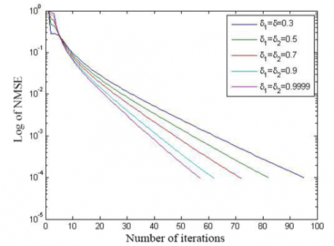
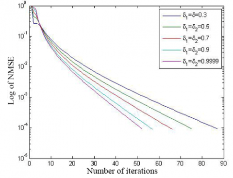
Firstly, the target signal was measured for 2N-1=101 times, that is, the Hankel matrix is of the dimension N=51; the rank R, and the size of location set Ω were set to 3 and 20, respectively. Then, the efficiency of signal recovery, i.e., the NMSE between initial and final matrices ( $\frac{\left\|H^{(f i n a l)}-\widetilde{H}\right\|_{2}}{\|\widetilde{H}\|_{2}}$ ≤0.0001) is reported in Figure 1.
(a) N=51, R=1, and M=10
(b) N=51, R=3, and M=20
Figure 1. The influence of δ1and δ2 on the convergence of the initial algorithm (simulation 1)
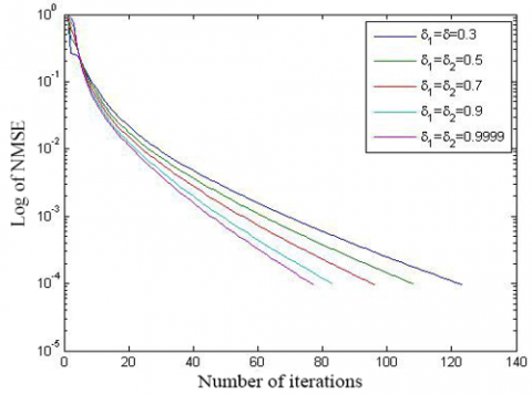
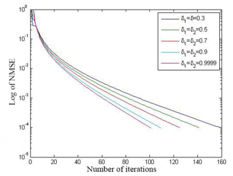
(a) N=501, R= 5, and M=100
(b) N=501, R=8, and M=200
Figure 2. The influence of δ1and δ2 on the convergence of the initial algorithm (simulation 2)
Secondly, the target signal was measured for 2N-1=5,001 times, that is, the Hankel matrix is of the dimension N=51; the rank R, and the size of location set Ω were set to 2,501 and 13, respectively. Then, the efficiency of signal recovery, i.e., the NMSE between initial and final matrices is reported in Figure 2.
After that, the recovery time of the signal with the initial algorithm with different parameters is displayed in Table 1. Obviously, the greater the parameter values, the smaller the NMSE, and the more efficient the signal recovery. Hence, the two parameters were set to 0.9999 for the following experiments.
Table 1. The recovery time of the signal with the initial algorithm with different parameters
|
Signal |
δ1,δ2=0.3 |
δ1,δ2=0.5 |
δ1,δ2=0.7 |
δ1,δ2=0.9 |
δ1,δ2=0.9999 |
|
N=51, R=1, M=10 |
0.55s |
0.49s |
0.43s |
0.36s |
0.34s |
|
N=51, R=3, M=20 |
0.72s |
0.64s |
0.58s |
0.50s |
0.46s |
|
N=501, R=5, M=100 |
20.17s |
17.85s |
15.84s |
13.89s |
12.69s |
|
N=501, R=8, M=200 |
10.97s |
9.52s |
8.29s |
7.06s |
6.67s |
4.2 Phase transition for precise recovery (PTPR)
To verify its feasibility, our algorithm was subject to multiple simulations on PTPR. A total of one hundred 100 Morte-Carlo simulations were conducted for each pair of R and M. Then, R frequencies were selected by random in the interval [0, 1), and used to produce a complex signal x with sparse spectrum. Then, the initial algorithm was implemented under δ1=δ2=0.9999. Each simulation was deemed as a success, provided that the NMSE meets $\left\|x^{(\text {final })}-\tilde{x}\right\|_{2} /\|\tilde{x}\|_{2} \leq 0.005$, with $\hat{\mathrm{X}}$ being the expected return of our algorithm. The final success rate was obtained as the mean of the 100 simulations.
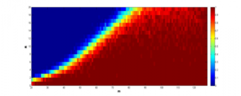
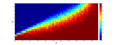
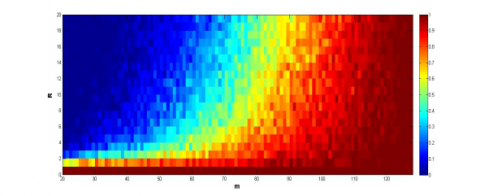
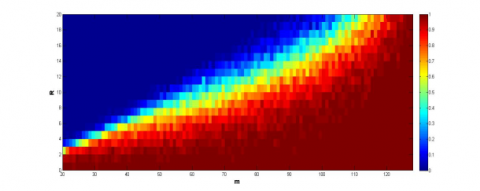
The simulation results on the signals with dimensions between 20 and 127 are recorded in Figure 3, where the y-axis is the number of samples, and the x-axis is the level of sparsity, and the color of each grid is the success rate. It can be seen that the initial algorithm and the speed-up strategy outshined the other algorithms, especially the speed-up strategy, in the effect and feasibility in signal recovery. The two algorithms can recover the signals with fewer samples than the other algorithms.
(a) PTPR of speed-up strategy
(b) PTPR of initial algorithm
(c) PTPR of ANM with $\Delta f>\frac{1.5}{\|\mathcal{N}\|}$
(d) PTPR of ANM without $\Delta f>\frac{1.5}{\|\mathcal{N}\|}$
(e) PTPR of EMaC
Figure 3. The PTPR of different algorithms
Note: The ANM and EMaC are short for atomic norm minimization [14], and enhanced matrix completion, respectively.
4.3 Speed up effect
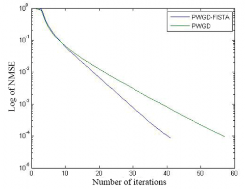
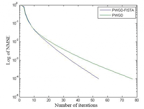
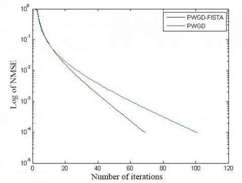
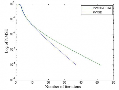
The convergence of initial algorithm is compared with the speed up strategy in Figures 4 and 5, and Table 2. It is obvious that the speed up strategy converged more rapidly than the initial algorithm. To reach the solution of comparable precision, the speed up strategy only needed two thirds the number of iterations of the initial algorithm.
(a) N=51, R=1, and M=10
(b) N=51, R=3,and M=20
Figure 4. The convergence curves of the two algorithms (simulation 3)
(a) N=501, R=8, and M=200
(b) N=5,001, R=20, and M=1,000
Figure 5. The convergence curves of the two algorithms (simulation 4)
Table 2. The convergence speeds of the two algorithms
|
Signal |
Speed up strategy |
Initial algorithm |
|
N=51, R=1, M=10 |
0.29s |
0.34s |
|
N=51, R=3, M=20 |
0.38s |
0.46s |
|
N=101, R=5, M=40 |
0.90s |
0.95s |
|
N=501, R=5, M=100 |
8.48s |
12.69s |
4.4 Recovery of large-dimensional 1D signal
Furthermore, the two proposed methods were compared with ANM and EMaC, two convex optimization strategy, to verify their effect on the recovery of large-dimensional 1D signals. Our methods were expected to work effectively on large signals with sparse spectrum. Our methods adopt the same settings as previously; the contrastive methods were solved by CVX software. Table 3 compares the recovery time of signals with different sizes. It can be seen that our methods recovered medium signals faster than the contrastive methods, and performed excellently on the recovery of large signals.
Table 3. The recovery time of signals with different sizes
|
Signals |
Speed up strategy |
Initial algorithm |
ANM |
EMaC |
|
N=51, R=1, M=10 |
0.29s |
0.34s |
5.7s |
47.8s |
|
N=51, R=3, M=20 |
0.38s |
0.46s |
6.9s |
58.0 |
|
N=101, R=5, M=40 |
0.90s |
0.95s |
51.6s |
787.6s |
|
N=501, R=5, M=100 |
8.48s |
12.69s |
N/A |
N/A |
|
N=2501, R=13, M=500 |
88.95s |
133.25s |
N/A |
N/A |
|
N=2501, R=25, M=1000 |
70.71s |
91.46s |
N/A |
N/A |
|
N=5001, R=20, M=1000 |
473.48s |
645.09s |
N/A |
N/A |
|
N=5001, R=31, M=2000 |
301.03s |
402.56s |
N/A |
N/A |
This paper presents a feasible-point algorithm for the recovery of signals with sparse spectrum, and continuous frequencies in the interval [0, 1], using only a few data in the time domain. Unlike the conventional recovery methods, the initial algorithm takes root in the non-convex optimization, and handles large-dimensional signals effectively. The convergence of the algorithm was verified through repeated simulations.
Moreover, the convergence of the initial algorithm was accelerated by referring to the FIST algorithm. Simulations show that the initial algorithm and the speed up strategy could recover signals on medium and large scales successfully from a limited amount of data in the time domain, and outperform contrastive methods like ANM and EMaC.
The future research will focus on the following aspects: identifying the theoretical limit on the sample size for signal recovery by our algorithms; applying our methods to the recovery of damped signals, e.g., the fluctuation GNP data; solving the problems in the programming of the Hankel matrix.
The research is supported by Scientific Research Project of Education Department of Hubei Province (Grant No.: Q20201510).
[1] Ledenyov, D., Ledenyov, V. (2015). Digital waves in economics. Available at SSRN 2613434. https://dx.doi.org/10.2139/ssrn.2613434
[2] Ledenyov, D., Ledenyov, V. (2015). On the spectrum of oscillations in economics. Available at SSRN 2606209. https://dx.doi.org/10.2139/ssrn.2606209
[3] Beck, A., Teboulle, M. (2009). A fast iterative shrinkage-thresholding algorithm for linear inverse problems. SIAM Journal on Imaging Sciences, 2(1): 183-202. https://doi.org/10.1137/080716542
[4] Cai, J.F., Qu, X., Xu, W., Ye, G.B. (2016). Robust recovery of complex exponential signals from random Gaussian projections via low rank Hankel matrix reconstruction. Applied and Computational Harmonic Analysis, 41(2): 470-490. https://doi.org/10.1016/j.acha.2016.02.003
[5] Tropp, J.A., Laska, J.N., Duarte, M.F., Romberg, J.K., Baraniuk, R.G. (2009). Beyond Nyquist: Efficient sampling of sparse bandlimited signals. IEEE Transactions on Information Theory, 56(1): 520-544. https://doi.org/10.1109/TIT.2009.2034811
[6] Yin, W., Osher, S., Goldfarb, D., Darbon, J. (2008). Bregman iterative algorithms for l1-minimization with applications to compressed sensing: SIAM Journal Imaging Sciences, 1: 143-168. https://doi.org/10.1137/070703983
[7] Bolte, J., Sabach, S., Teboulle, M. (2014). Proximal alternating linearized minimization for nonconvex and nonsmooth problems. Mathematical Programming, 146(1-2): 459-494. https://doi.org/10.1007/s10107-013-0701-9
[8] Cai, J.F., Osher, S., Shen, Z. (2009). Linearized Bregman iterations for compressed sensing. Mathematics of Computation, 78(267): 1515-1536. https://doi.org/10.1090/S0025-5718-08-02189-3
[9] Sarkar, T.K., Pereira, O. (1995). Using the matrix pencil method to estimate the parameters of a sum of complex exponentials. IEEE Antennas and Propagation Magazine, 37(1): 48-55. https://doi.org/10.1109/74.370583
[10] Chandrasekaran, V., Recht, B., Parrilo, P.A., Willsky, A.S. (2012). The convex geometry of linear inverse problems. Foundations of Computational Mathematics, 12(6): 805-849. https://doi.org/10.1007/s10208-012-9135-7
[11] Candès, E.J., Fernandez-Granda, C. (2014). Towards a mathematical theory of super-resolution. Communications on Pure and Applied Mathematics, 67(6): 906-956. https://doi.org/10.1002/cpa.21455
[12] Daubechies, I., Defrise, M., De Mol, C. (2004). An iterative thresholding algorithm for linear inverse problems with a sparsity constraint. Communications on Pure and Applied Mathematics: A Journal Issued by the Courant Institute of Mathematical Sciences, 57(11): 1413-1457.
[13] Candès, E.J., Romberg, J., Tao, T. (2006). Robust uncertainty principles: Exact signal reconstruction from highly incomplete frequency information. IEEE Transactions on Information Theory, 52(2): 489-509. https://doi.org/10.1109/TIT.2005.862083
[14] Xu, W., Cai, J.F., Mishra, K.V., Cho, M., Kruger, A. (2014). Precise semidefinite programming formulation of atomic norm minimization for recovering d-dimensional (d≥2) off-the-grid frequencies. In 2014 Information Theory and Applications Workshop (ITA), pp. 1-4. https://doi.org/10.1109/ITA.2014.6804267
[15] Tang, G., Bhaskar, B.N., Recht, B. (2013). Sparse recovery over continuous dictionaries-just discretize. In 2013 Asilomar Conference on Signals, Systems and Computers, pp. 1043-1047. https://doi.org/10.1109/ACSSC.2013.6810450
[16] Candès, E.J., Recht, B. (2009). Exact matrix completion via convex optimization. Foundations of Computational Mathematics, 9(6): 717. https://doi.org/10.1007/s10208-009-9045-5
[17] Chen, Y., Chi, Y. (2013). Spectral compressed sensing via structured matrix completion. arXiv preprint arXiv:1304.4610.
[18] Attouch, H., Bolte, J., Redont, P., Soubeyran, A. (2010). Proximal alternating minimization and projection methods for nonconvex problems: An approach based on the Kurdyka-Łojasiewicz inequality. Mathematics of Operations Research, 35(2): 438-457. https://doi.org/10.1287/moor.1100.0449
[19] Lustig, M., Donoho, D., Pauly, J.M. (2007). Sparse MRI: The application of compressed sensing for rapid MR imaging. Magnetic Resonance in Medicine: An Official Journal of the International Society for Magnetic Resonance in Medicine, 58(6): 1182-1195. https://doi.org/10.1002/mrm.21391
[20] Cai, J.F., Liu, S., Xu, W. (2015). A fast algorithm for reconstruction of spectrally sparse signals in super-resolution. In Wavelets and Sparsity XVI. pp. 70-76. https://doi.org/10.1117/12.2188489
[21] Tang, G., Bhaskar, B.N., Shah, P., Recht, B. (2013). Compressed sensing off the grid. IEEE Transactions on Information Theory, 59(11): 7465-7490. https://doi.org/10.1109/TIT.2013.2277451
[22] Cai, J.F., Osher, S., Shen, Z. (2009). Convergence of the linearized Bregman iteration for ℓ₁-norm minimization. Mathematics of Computation, 78(268): 2127-2136. https://doi.org/10.1090/S0025-5718-09-02242-X
[23] Toh, K.C., Todd, M.J., Tütüncü, R.H. (1999). SDPT3-A MATLAB software package for semidefinite programming, version 1.3. Optimization Methods and Software, 11(1-4): 545-581. https://doi.org/10.1080/10556789908805762
[24] Cai, J.F., Candès, E.J., Shen, Z. (2010). A singular value thresholding algorithm for matrix completion. SIAM Journal on Optimization, 20(4): 1956-1982. https://doi.org/10.1137/080738970
[25] Blumensath, T., Davies, M.E. (2009). Iterative hard thresholding for compressed sensing. Applied and Computational Harmonic Analysis, 27(3): 265-274. https://doi.org/10.1016/j.acha.2009.04.002
[26] Jain, P., Meka, R., Dhillon, I. S. (2010). Guaranteed rank minimization via singular value projection. In Advances in Neural Information Processing Systems, pp. 937-945.
[27] Fischer, R.F. (2005). Precoding and Signal Shaping for Digital Transmission. John Wiley & Sons.
[28] Golub, G.H., Van Loan, C.F. (2013). Matrix Computations (4th ed.). The Johns Hopkins University Press.
[29] Borcea, L. (2001). Interferometric imaging and time reversal in random media. Encyclopedia of Applied and Computational Mathematics, pp. 697-705. https://doi.org/10.1007/978-3-540-70529-1_157
[30] Scharf, L.L. (1991). Statistical Signal Processing. Reading, MA: Addison-Wesley.
[31] Roy, R., Kailath, T. (1989). ESPRIT-estimation of signal parameters via rotational invariance techniques. IEEE Transactions on Acoustics, Speech, and Signal Processing, 37(7): 984-995. https://doi.org/10.1109/29.32276
[32] Donoho, D.L. (2006). Compressed sensing. IEEE Transactions on Information Theory, 52(4): 1289-1306. https://doi.org/10.1109/TIT.2006.871582
[33] Chi, Y., Scharf, L.L., Pezeshki, A., Calderbank, A.R. (2011). Sensitivity to basis mismatch in compressed sensing. IEEE Transactions on Signal Processing, 59(5): 2182-2195. https://doi.org/10.1109/TSP.2011.2112650
[34] Fazel, M., Pong, T.K., Sun, D., Tseng, P. (2013). Hankel matrix rank minimization with applications to system identification and realization. SIAM Journal on Matrix Analysis and Applications, 34(3): 946-977. https://doi.org/10.1137/110853996